Transactive Energy Challenge Phase II Scenario - NIST Technical Note 2021 David Holmberg Martin Burns Steve Bushby Avi Gopstein - NIST ...

NIST Technical Note 2021

Transactive Energy Challenge
 Phase II Scenario
 David Holmberg
 Martin Burns
 Steve Bushby
 Avi Gopstein

 This publication is available free of charge from:
 https://doi.org/10.6028/NIST.TN.2021

NIST Technical Note 2021

 Transactive Energy Challenge
 Phase II Scenario

 David Holmberg1
 Martin Burns2
 Steven Bushby1
 Avi Gopstein2
 1
 Energy and Environment Division
 2
 Smart Grid Program Office
 Engineering Laboratory

 This publication is available free of charge from:
 https://doi.org/10.6028/NIST.TN.2021

 October 2018

 U.S. Department of Commerce
 Wilbur L. Ross, Jr., Secretary

 National Institute of Standards and Technology
Walter Copan, NIST Director and Undersecretary of Commerce for Standards and Technology

Certain commercial entities, equipment, or materials may be identified in this
 document in order to describe an experimental procedure or concept adequately.
 Such identification is not intended to imply recommendation or endorsement by the
 National Institute of Standards and Technology, nor is it intended to imply that the
 entities, materials, or equipment are necessarily the best available for the purpose.

National Institute of Standards and Technology Technical Note 2021
Natl. Inst. Stand. Technol. Tech. Note 2021, 18 pages (October 2018)
 CODEN: NTNOEF

 This publication is available free of charge from:
 https://doi.org/10.6028/NIST.TN.2021

ABSTRACT
 The Transactive Energy (TE) Challenge Phase II Scenario was developed in a multi-step
 process in collaboration with industry experts. The Scenario enables comparison of results
 from different TE simulations and different TE approaches. The Scenario includes a common
 electric grid definition including attached loads and generators, weather, and reporting
 metrics. This document and the files that it references serve as a repository for future use.

 Key words
This publication is available free of charge from: https://doi.org/10.6028/NIST.TN.2021

 co-simulation; high-penetration PV; modeling; transactive energy; use case scenarios;
 voltage control

 i

Table of Contents
 Introduction ..................................................................................................................... 1
 Common Scenario components ...................................................................................... 1
 2.1. IEEE 8500 Grid ........................................................................................................... 1
 2.2. Weather scenario ......................................................................................................... 3
 2.3. Team Simulations ........................................................................................................ 3
 2.4. Price data ..................................................................................................................... 4
This publication is available free of charge from: https://doi.org/10.6028/NIST.TN.2021

 2.5. Common Metrics ......................................................................................................... 5
 Conclusion ........................................................................................................................ 6
 References ................................................................................................................................ 7
 Appendix: Development of the TE Challenge Phase II Scenario ....................................... 8

 ii

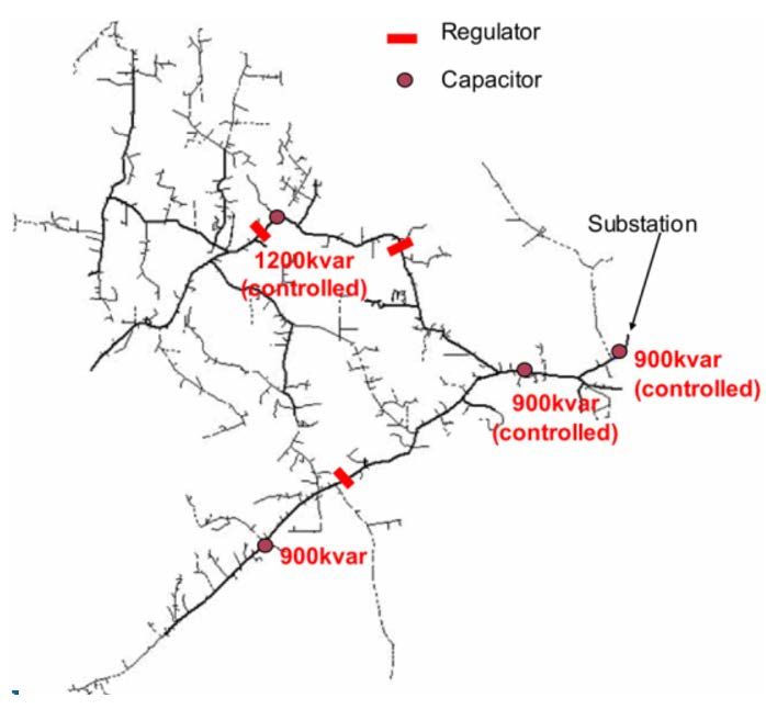
Introduction
 The TE Challenge Phase II focused on a TE co-simulation exercise based on a
 collaboratively developed common scenario, including metrics, that advanced the goals of
 the Challenge [1, 2, 3]. The first goal of Phase II was to perform TE simulations using a
 collaboratively developed TE scenario that serves as a baseline for comparisons of simulation
 results. Using a common electric grid, weather, loads, and reporting metrics enables the
 direct comparison of results from different TE simulations and different TE approaches. This
 document and the files that it references serve as a repository for future use.
 Common scenarios are important tools for understanding and describing the value of various
This publication is available free of charge from: https://doi.org/10.6028/NIST.TN.2021

 TE components and strategies. Defining use cases with specific objectives allows the
 effectiveness of TE solutions to be analytically compared against business-as-usual or
 baseline scenarios. To facilitate meaningful comparison across strategies, use cases must
 include common reference grids, environmental conditions, and objectives.

 Developing the common scenario began in Phase I of the Challenge [3] with development of
 a set of transactive energy use cases, and then selection and development of one of those use
 cases for further modeling work. The process and details of that effort are documented in the
 Appendix. Prior to the Phase II launch, NIST worked with Pacific Northwest National
 Laboratories (PNNL), Vanderbilt University, and Carnegie Mellon University to further
 develop the TE Challenge Phase II strawman scenario components. This strawman scenario
 and a proposed scenario development process [4] were shared during the April 2017 Phase II
 Launch. The Challenge scenario was then refined with Phase II teams over a series of web
 conferences and a face-to-face meeting in the months of May and June 2017. Some
 additional modifications were made as the Challenge progressed. The final simulation
 components of the Challenge scenario are hosted online [5].
 The Challenge Scenario is a collection of components including: a specific electric feeder
 with specified loads and generators, an event sequence (weather for one day), a time-of-use
 price schedule for the baseline (non-TE) case, a series of simulations that range from a non-
 TE baseline to simulations with TE models chosen by each team, and an agreed upon set of
 common metrics for reporting results. These components are discussed more below.
 Common Scenario components
 Several factors guided the selection of weather, grid and other components. It was initially
 agreed to focus on the distribution grid as an appropriate place to investigate transactive
 energy with grid-edge market interactions. The target use case focused on voltage control due
 to high-penetration of photovoltaic (PV) systems. A large feeder model was chosen to
 provide diversity of loads and generation with potential for voltage variation across the
 feeder due to the concentration of PV generation. To reduce complexity of the co-simulation
 exercise, teams agreed not to model the transmission grid.

 2.1. IEEE 8500 Grid
 The Institute of Electrical and Electronics Engineers (IEEE) 8500 reference distribution grid
 [6], shown in Fig. 1, was selected as the basis for the Challenge scenario. This 8500-node test
 feeder is a moderately large radial distribution feeder consisting of both low and medium

 1

voltage (MV) levels. The nodes occur at approximately 4,800 1-, 2-, and 3-phase bus
 locations. The power flow is moderately difficult to solve at the specified load level. The test
 grid also exhibits approximately 10 % power losses at peak load. The circuit contains 170 km
 of primary (MV) conductor. The circuit contains one set of regulators controlling the feeder
 voltage at the substation and three sets of voltage regulators along the line. The circuit also
 contains four capacitor banks, three that include per-phase capacitor control. The controlled
 capacitor banks monitor each phase separately, and each capacitor bank operates the
 respective capacitor on the same phase. The capacitor switches ON when the reactive power
 flow in the line is 50 % of the capacitor size and switches OFF when the flow is 75 % of the
 capacitor size in the reverse direction. Each controlled capacitor also includes voltage
This publication is available free of charge from: https://doi.org/10.6028/NIST.TN.2021

 override where the capacitor turns ON at 0.9875 pu and turns OFF at 1.075 pu.
 The test feeder makes two load model cases (secondary loading case models with residential
 loads connected to a 120V/240V split-phase transformer in balanced and unbalanced
 configurations) available to users. The teams agreed to use a balanced configuration.
 Specifications for loads, PV generation, and batteries in houses at each meter were
 developed. As specified, the grid is a purely residential feeder, with a nominal peak load of
 10.8 MW and 2.7 MVAr. Of the 1,977 houses on the feeder, all of them were configured
 with air conditioning (26.15 MW load), and 90 % (1,777) of them with PV systems with total
 peak solar production of 6,755 kW. In addition, 857 homes have batteries with a total storage
 capacity of 4,285 kW (although these were not used in the baseline configuration), and 1,013
 homes have electric water heaters totaling 4,574 kW. The grid definition and specific details
 of each house (thermal parameters and equipment), are contained in the inv8500.glm
 GridLab-D model file, available on a GitHub site managed by PNNL as part of their TE
 Simulation Platform (TESP) [7]. TE Challenge scenario files are maintained within the
 /examples/IEEE8500 directory of TESP Release 1.1 [5]. This directory has a readme.md file
 that explains the various model files, input files, data processing scripts, and results files.
 This directory serves as a repository of the TE Challenge scenario simulation files.

 2

This publication is available free of charge from: https://doi.org/10.6028/NIST.TN.2021

 Figure 1 IEEE 8500 grid schematic.

 2.2. Weather scenario
 The High-penetration PV and Voltage Control scenario (refer to the Appendix for more
 detail) was originally written for a distribution system with a high penetration of PV systems
 and over-voltage conditions under sunny skies. The TE Challenge teams agreed to add a
 storm passing to induce voltage fluctuations and then to use transactive methods to
 incentivize controlled changes in load, generation or storage to mitigate the voltage
 imbalances. The single day scenario begins with clear sky conditions followed by PV
 generation dropping from full power to 10 % power output in the 2:30 p.m. to 2:40 p.m. time
 window due to the storm front arrival. The overcast conditions last until a ramp back up to
 full sun from 4:00 p.m. to 4:30 p.m.
 This scenario narrative is realized in simulation using the climate.csv weather input file [5]
 based on a sunny Tucson weather day with the addition of an artificial storm front per the
 narrative above. There is no time shift for the storm front passing over the feeder; every PV
 panel sees the same weather at the same time per above.

 2.3. Team Simulations
 Teams followed an implementation plan with four simulations in a progression to allow
 building up common understanding, validation by comparison of results, and refinement of
 the scenario components themselves. The progressive simulations were:
 1. Baseline sunny day. The event day is run with no storm front. Electricity price is
 constant with no TE market interactions.

 3

2. Adding the storm front. Simulation is repeated with the storm front weather file,
 with all else the same.
 3. Adding dynamic price, without TE market. Teams may enable resources to be
 price responsive, but there are no TE exchanges.
 4. Each team implements a TE model of their choice and applies it to the same
 feeder and weather event.

 2.4. Price data
 Teams agreed to use existing Tucson Electric retail tariffs and representative Tucson
 locational marginal pricing (LMP) data for a summer day. The Residential Basic Service flat
This publication is available free of charge from: https://doi.org/10.6028/NIST.TN.2021

 rate tariff [9] was used for simulation Steps 1 and 2, with components given in Table 1. The
 resulting “fixed rate” value used in the one-day TE Challenge simulation, 0.102 $/kWh, is
 the sum of the 0 to 500 kWh Energy Service Charge plus the Power Supply Charge.

 Table 1 Tucson Electric Residential Basic Service Tariff
 Tariff Component Charge Range
 Basic Service Fee $13.00
 Energy Service $0.066152/kWh (0 to 500) kWh
 $0.081152/kWh (501 to 1000) kWh
 $0.086652/kWh Over 1000 kWh
 Power Supply $0.035861/kWh Summer value

 The Residential Time-of-Use (TOU) rate [10] was used for Step 3. The TOU rate
 components are given in Table 2. For TE Challenge simulations, the on-peak or off-peak
 Power Supply Charge is added to the Energy Service Charge component.

 Table 2 Tucson Electric Residential Service Time-of-Use Tariff
 Tariff Component Charge Range
 Basic Service Fee$10.00
 Energy Service $0.072152/kWh (0 to 500) kWh
 $0.081152/kWh (501 to 1000) kWh
 $0.086652/kWh Over 1000 kWh
 Power Supply $0.066567/kWh On-peak*
 $0.026332/kWh Off-peak
 * Summer On-Peak period is 3:00 p.m. to 7:00 p.m., Monday through Friday.

 For PNNL TESP Gridlab-D users, the flat price and TOU tariffs are embedded in the GLM
 file. One can switch between basic and TOU by commenting/uncommenting near the top of
 the file, and all the meters reference those tariff schedules. LMP five-minute clearing price
 data [11] are based on the California Independent Service Operator real-time market prices
 for Tucson 1 for July 6, 2017, which has base prices around $20/MWh and peaks around

 1
 Taken from oasis.caiso.com Prices/Interval Locational Marginal Price at load node SG_LNODE13A.

 4

$50/MWh in the afternoon. Day-ahead market hourly LMPs are also available for July 6-7 2.
 Use of the LMP real-time or day-ahead data is not required.

 2.5. Common Metrics
 To promote the ability to compare the results from simulations using different TE market and
 control approaches, the participating teams agreed to a set of common performance metrics.
 The metrics were derived from features of the PNNL TESP, American National Standards
 Institute (ANSI) C84.1 [12], and IEEE 1366 [13]. Teams were permitted to ignore metrics
 not applicable to their simulations and to use additional metrics relevant to their results.
This publication is available free of charge from: https://doi.org/10.6028/NIST.TN.2021

 General guidelines:
 • Save results in a text format, JavaScript Object Notation (JSON) (preferred) or
 common-separated values (CSV)
 • Adjustable metrics interval, defaulting one minute
 • If the simulation time step is shorter than the metrics interval, include minimum,
 maximum and average values within each interval. Integrated metrics (e.g., energy)
 are an exception
 • Optionally, save all power flow data to CSV files by manually inserting recorder
 statements in the GridLab-D input file
 • Separate PV output, battery, and load metrics at the same meter
 • No time aggregation, as the use case covers a single day of operation
 • Each metric should be associated with specific model components through metadata
 • All measurements are time stamped

 Specific requirements for base metrics to include in the output:
 1. Economic
 a. Wholesale price (defaults to the input LMP player file)
 b. Cleared price(s) on the feeder
 c. Price, quantity, and status (accepted, not accepted) for each bid
 d. Revenue at each meter, separable by load and resource (see 4.f-k,m below)
 2. Substation
 a. Real and reactive power
 b. Real and reactive energy
 c. Real and reactive losses
 3. At each feeder capacitor bank and voltage regulator
 a. Count of control actuations
 4. At each meter (i.e., house)
 a. Voltage magnitude, line-to-neutral, averaged over all phases
 b. Voltage magnitude, line-to-line, averaged over all phases 3

 2
 Taken from oasis.caiso.com Prices/Locational Marginal Prices with DAM option and SG_LNODE13A
 selected.
 3
 Because of the use of the balanced-secondary version of the IEEE 8500-node feeder, there is no secondary
 voltage unbalance at single-phase loads. The normalized line-to-neutral and line-to-line voltage magnitudes are
 equal. For such single-phase loads, Vavg should be defined on a 120 V basis.

 5

c. For three-phase loads only, line-to-line voltage imbalance as defined in ANSI
 Standard C84.1: 100 max (| − |)⁄ [%], where Vp = phase voltage,
 =1..3
 and Vavg is the average of the three phases.
 d. Severity index (SI) for the fluctuation in Vavg on per-unit basis at uniform time
 step. Similar to an L2 norm; = ∑ =1 �( − −1 )2 + 1 . This metric has
 also been used to quantify fluctuations in solar irradiance. IEEE 1453 is less
 applicable because cloud-induced fluctuations are generally too slow.
 e. Violations of ANSI C84.1 voltage limits at the meter. The duration of time in
 each range should be accumulated. An event count occurs when the voltage
This publication is available free of charge from: https://doi.org/10.6028/NIST.TN.2021

 transitions from normal to A Range, or from A Range to B Range.
 i. Total duration and event counts below 110 V (B Range)
 ii. Total duration and event counts below 114 V (A Range)
 iii. Total duration and event counts above 126 V (A Range)
 iv. Total duration and event counts above 127 V (B Range)
 v. Total duration and event counts below 10 V (Outage; none expected)
 f. Total house load (real power)
 g. Total heating ventilation air conditioning (HVAC) load (real power)
 h. Total water heater load (real power)
 i. Solar inverter real and reactive power
 j. Battery inverter real and reactive power
 k. House air temperature, and its deviation from scheduled set point evaluated
 by:
 i. Root mean squared deviation
 ii. Maximum deviation
 iii. Duration, average magnitude, and direction of the longest excursion
 l. Water heater temperature and its deviation from scheduled set point
 m. Total bill synchronized to the cleared market price 4
 5. Local utilization of green power, defined as the percentage of locally-generated green
 energy in the total energy consumed by all the customers connected to a feeder or in a
 microgrid. The sources of green energy considered are roof-top solar PV, but not
 batteries.
 Conclusion
 The TE Challenge Phase II common scenario is a collection of components including grid
 and weather definition, common metrics and progressive simulation plan. The scenario was
 developed collaboratively by the TE Challenge teams, with significant input from PNNL for
 definition of homes and metrics, and providing the grid definition in GridLab-D format. This
 paper and the PNNL GitHub repository of technical files serves to document this reference
 scenario so that others can duplicate and use the scenario for comparative TE simulations.

 4
 The 8500-node model as implemented here assumes net metering, with distributed energy resource (DER)
 disaggregation based on real power. An alternative would be to meter each DER separately from the house, so
 each could have its own tariff and bill.

 6

References
 [1] D.G. Holmberg, M. Burns, et.al., “NIST Transactive Energy Modeling and Simulation
 Challenge Phase II Report,” NIST Spec. Pub. 1900-603, available from:
 https://doi.org/10.6028/NIST.SP.1900-603, 2018.
 [2] NIST TE Challenge website. https://www.nist.gov/engineering-laboratory/smart-grid/hot-
 topics/transactive-energy-modeling-and-simulation-challenge.
 [3] D.G. Holmberg, S.T. Bushby, “NIST Transactive Energy Modeling and Simulation
 Challenge for the Smart Grid—Phase I Report,” NIST Tech. Note 2019, available from:
 https://doi.org/10.6028/NIST.TN.2019, 2018.
This publication is available free of charge from: https://doi.org/10.6028/NIST.TN.2021

 [4] NIST TE Challenge Phase II Collaborative Scenario Development (2017).
 https://s3.amazonaws.com/nist-
 sgcps/TEChallenge/Library/TECCollabScenDevp20170420.docx.
 [5] PNNL TE Challenge scenario repository in TESP Release 1.1 (2018). Available:
 https://github.com/pnnl/tesp/releases/tag/v0.1.1.
 [6] Arnatt D (2010) The IEEE 8500-node test feeder, Transmission and Distribution
 Conference and Exposition, IEEE PES. DOI: 10.1109/TDC.2010.5484381, and grid
 component files at: https://ewh.ieee.org/soc/pes/dsacom/testfeeders/8500node.zip
 [7] PNNL TE Simulation Platform http://tesp.readthedocs.io/.
 [8] Holmberg D, Hardin D, Cunningham R, Melton R, Widergren S (2016) “Transactive
 Energy Application Landscape Scenarios,” SGIP Technical Paper.
 http://www.sgip.org/wp-
 content/uploads/SGIP_White_Paper_TE_Application_Landscape_Scenarios_12-15-
 2016_FINAL.pdf .
 [9] Tucson Electric Residential Basic Service (2018) https://www.tep.com/wp-
 content/uploads/2017/02/101-TRRES.pdf.
 [10] Tucson Electric Residential Time-of-Use (2018) https://www.tep.com/wp-
 content/uploads/2017/02/102-TRREST.pdf.
 [11] CAISO real-time market prices for July 6, 2017, Tucson LMP five-minute clearing price
 data (2017) https://github.com/pnnl/tesp/blob/master/examples/players/lmp_value.csv.
 [12] ANSI C84.1-1982. American National Standard for Electric Power Systems and
 Equipment-Voltage Ratings (60Hz).
 [13] IEEE 1366-2012 - IEEE Guide for Electric Power Distribution Reliability Indices.
 [14] Burns, M., Song, E., Holmberg, D., The Transactive Energy Challenge Abstract
 Component Model, NIST Special Pub 1900-602, available from:
 https://doi.org/10.6028/NIST.SP.1900-602, 2018.

 7

Appendix: Development of the TE Challenge Phase II Scenario

 The TE Challenge Phase II Scenario development proceeded over the course of more than a
 year. The initial work began with the definition of six transactive energy use case scenarios
 [8] which grew out of the TE Challenge Phase I work. Near the end of Phase I, a focused
 effort was initiated to develop a common TE abstract model [14]. The development of the TE
 abstract model began with a meeting on June 23, 2016 with experts from National Institute of
 Standards and Technology (NIST), Department of Energy (DOE), Pacific Northwest
 National Laboratory (PNNL), Vanderbilt University, and Carnegie Mellon University
This publication is available free of charge from: https://doi.org/10.6028/NIST.TN.2021

 (CMU). Experts at this meeting noted that a detailed test scenario would be needed to
 demonstrate and validate this TE abstract model. To that end, the experts analyzed the six TE
 use case scenarios according to a set of criteria to identify a single use case which became the
 basis for the TE Challenge Phase II scenario. Beyond this, they considered a phased approach
 for increasing the complexity of the use case from a simplistic grid model with baseline
 conditions to a more realistic grid and environmental conditions.

 This appendix begins with a short review of the six use cases, followed by the assessment
 and prioritization of the use cases against a set of criteria, leading to the selection of the
 High-penetration PV and Voltage Control scenario for use in simulations. The initial
 thoughts on the phased use case development are also documented.

 Phase I Use Cases
 During Phase I of the TE Challenge, one of the teams focused on developing a reference grid
 design and interoperability requirements to allow testing of different TE approaches for a set
 of scenarios. That team contributed to a white paper [8] which identified six core use cases
 (UCs) for TE assessment:

 • UC1: Peak Heat Day and Energy Supply;
 • UC2: Wind Energy Balancing Reserves;
 • UC3: High-Penetration PV and Voltage Control;
 • UC4: EVs on the Neighborhood Transformer;
 • UC5: Islanded Microgrid Energy Balancing; and
 • UC6: System Constraint Resulting in Mandatory Curtailment.

 The six use cases represent a diverse set of modeling, environmental, economic, and
 operational considerations. While each of the use cases represents an interesting scenario and
 value proposition for TE approaches, there is some overlap of the objectives across use cases.
 Additionally, given the state of model capability, it is not currently possible to transparently
 evaluate all the use cases.

 Use Case Assessment and Prioritization
 At the June 23 meeting of TE modeling experts, the six use cases were qualitatively assessed
 for prioritization. Because the value of TE assets are maximized in scenarios that require
 regular and ongoing optimization, use cases with objectives characterized by infrequent or
 emergency implementation of TE services (UC1 and UC6) were deemed to be of limited

 8

value in assessing early deployment scenarios for developing TE strategies. Furthermore,
 because emergency grid conditions are typically characterized by supply constraints and an
 associated need for load curtailment—as is the case in both UC1 and UC6—the team agreed
 that scenarios characterized by infrequent or emergency use cases do not provide materially
 different insight into TE operations than would other demand response scenarios.

 To assess the remaining scenarios, the team developed a set of five qualitative criteria.
 These criteria were simplicity, impact, advancement, modeling challenges, and utility
 relevance:
This publication is available free of charge from: https://doi.org/10.6028/NIST.TN.2021

 Simplicity – The ease with which scenario boundaries can be described, and impacts
 can be quantified. use cases focused on localized effects tended to score higher in this
 assessment, while use cases that required integration and overlap of bulk and
 distribution markets and/or operations tended to score lower due to the associated
 operational, regulatory, and economic uncertainty.

 Impact – The extent to which successful mitigation of the concern identified in the
 UC would fundamentally alter grid operational or infrastructure investment
 paradigms. use cases that would facilitate greater system flexibility and higher
 utilization rates for a broad set of existing grid assets tended to score higher in this
 assessment.

 Advance TE Frontier – The likelihood that data and knowledge produced by
 analyzing the UC would provide new and meaningful insight into TE business
 models, technologies, or operations. use cases focused on single asset functionality
 tended to score lower in this assessment.

 Exercise the Model Environment – The extent to which multiple tools would be
 required to work in parallel to assess solutions. use cases that focused on multiple
 spatial and temporal scales tended to score higher in this assessment.

 Interest by Utilities – The extent to which the UC could address high-priority
 operational concerns for utilities.5

 Experts at the June 23 meeting scored the use cases via two approaches (see Table A-1). Use
 cases were first graded independently for each of the criteria with numerical scores of 1, 2 or
 3 assigned for grades of good, neutral, or bad (respectively), shown as “Absolute Grading” in
 Table A-1. The intention was to provide some assessment of the absolute value for each use
 case. There was no restriction on applying the same score for a given criterion to multiple use
 cases.

 Next, the use cases were compared and assigned an ordinal priority for each evaluation
 criterion (“Relative Ranking” in Table A-1). This was intended to provide some assessment
 of the relative value and ease of implementation of the use cases.

 5
 No utility representatives participated in the June 23, 2016 meeting, although many meeting
 participants had extensive experience working for and collaborating with electric utilities.

 9

Table A-1 Ranking use cases.
 Absolute Grading Relative Ranking
 UC2 UC3 UC4 UC5 UC2 UC3 UC4 UC5
 Simplicity 3 1 1 2 4 2 1 3
 Impact 1 2 3 1 1 2 4 3
 Advance TE Frontier 2 1 2 2 3 1 4 2
 Exercise Model Env. 1 2 3 2 1 3 4 2
 Interest by Utilities 1 1 3 2 1 2 4 3
 Total 8 7 12 9 10 10 17 13
This publication is available free of charge from: https://doi.org/10.6028/NIST.TN.2021

 It turned out that both methods resulted in the same prioritization of the use cases as shown
 in Table A-2.

 Table A-2 Use Case Prioritization
 Final Position Absolute Grading Method Relative Ranking Method
 1 High Penetration PV + VC High Penetration PV + VC
 2 Wind Balancing Reserves Wind Balancing Reserves
 3 Islanded Microgrid Energy Bal. Islanded Microgrid Energy Bal.
 4 EVs on Neighborhood Trans. EVs on Neighborhood Trans.

 Not prioritized Peak Heat Day Energy Supply Peak Heat Day Energy Supply
 Not prioritized System Constraint/Curtailment System Constraint/Curtailment

 Both UC3 (High-Penetration PV and Voltage Control) and UC2 (Wind Energy Balancing
 Reserves) received high marks at the experts meeting, although not without qualification.
 While the high PV scenario (UC3) was the top scorer, that relative ranking was in part driven
 by the high modeling complexity of, and therefore poor “simplicity” scores assigned to, the
 regional wind energy balancing scenario (UC2). As multi-scale models advance, perhaps
 through implementation of a TE co-simulation platform, and interactions across markets and
 economic incentives become better defined, the priority use case might switch from localized
 PV to regional wind integration.

 Experts noted that UC3 focuses on PV over-generation, and thus the need for load increase.
 This runs counter to the majority of early deployments of unconventional distributed energy
 resources which incorporate some form of infrastructure or energy constraint. 6,7,8 To provide
 greatest relevance from the analytic exercise, the prioritized TE Challenge analysis scenario

 6
 Olympic Peninsula Project
 (http://www.pnl.gov/main/publications/external/technical_reports/PNNL-17167.pdf)
 7
 Brooklyn Queens Demand Management (BQDM) Program
 (https://assets.documentcloud.org/documents/2782996/BQDM-Update-1-2016.pdf)
 8
 Phase 1 of CAISO’s Distributed Energy Resources proxy demand resource markets focused “solely
 on demand reduction, rather than… on both reducing and increasing demand.” (Source:
 https://www.caiso.com/Documents/RevisedStrawProposal_EnergyStorage_DistributedEnergyResour
 cesPhase2.pdf)

 10

must therefore broaden beyond demand inducement to include increasing measures of system
 flexibility. This concern was addressed in the TE Challenge Phase II Scenario with the
 introduction of a storm front.

 Use Case Definition
 The decision was then made that the TE Challenge-modeled use case(s) would focus on the
 impacts that high-penetrations of rooftop PV have on the distribution grid. Initial models
 would explore energy and power flow management over time by including a time-varying
 but spatially uniform resource curve. And as practical, geospatial resolution would be made
 finer and the resource modeled as temporally stochastic and spatially heterogeneous. The
This publication is available free of charge from: https://doi.org/10.6028/NIST.TN.2021

 June 23 meeting envisioned a phased approach to model complexity which would facilitate
 progressively more complex analysis and understanding of transactive approaches to
 optimize operations and markets that begin with energy and infrastructure management and
 grow to include ancillary services and stability issues.

 The following use case parameters were discussed. The agreed-on plan was that PNNL
 experts would fully define details of the model.

 • Grid conditions:
 o Single radial feeder to emphasize local effects. Beta version of feeder will be a
 four-node feeder, including:
  1 node for substation
  3 nodes for service transformers, each connected to 10 houses
 o Aggregate distributed rooftop PV capacity exceeds instantaneous demand by
 20 % at peak insolation. Distribution and capacity of PV to be determined by
 PNNL.
 o System shall remain in compliance with feeder capacity constraint, as defined
 by the reference grid; feeder capacity constraints to be modeled from IEEE
 8500 Node Test Feeder [6] to facilitate future scenario expansion.

 • Environmental conditions:
 o Resource: uniform sunshine, no clouds (clouds to be inserted in future
 iterations)
 o Suggested location and season: Spring in Southern California, determined to
 maximize the compound net load ramp as sun sets and demand peaks, while
 providing greatest flexibility to advance the scenario complexity as issues like
 regional balancing and integration are introduced.

 • Performance objectives:
 o Requirement 1: Minimize reverse power flows at feeder substation at peak PV
 generation
 o Requirement 2: Meet a scheduled load program throughout the day
  Initially, load program to be set for single model node (e.g., the feeder
 substation). As the scenario progresses beyond the beta example, load
 programs can be implemented at substation, regulators, or service
 transformers.

 11

• Customers, loads, and PV distribution:
 o 30 customers (beta model). Each customer load will be aggregated at the
 building level and consist of a number of representative systems and load
 profiles, including:
  HVAC;
  Lighting;
  Water heating;
  Miscellaneous electric loads;
  PV array (if appropriate, see below); and
This publication is available free of charge from: https://doi.org/10.6028/NIST.TN.2021

  Battery storage system (if appropriate).
 o PV deployments distributed so that total peak output is 120 % of peak
 demand.
 o Aggregate net customer loads to be reported at the building level

 • TE market model:
 o Depends on modeler

 • Analytics:
 o Not decided

 • Simplified behavior models:
 o Common customer load profile schedule default for each load category
 o PV conversion efficiency
 o Weather model provides insolation vs. time
 o Common customer price responsiveness for each load category

 Planned Use Case development approach
 The sample 30-house feeder described above was envisioned as a beta formulation meant to
 demonstrate the functionality of a TE modeling platform. Following demonstration of co-
 simulation analysis on this simple feeder, the model would be progressively modified to
 properly reflect real-world grid complexities. Building from the 4-node, 30-customer feeder
 described above, progressive expansion of the sample feeder would include:

 • Node/customer expansion:
 o Intermediate model: 50 nodes, 400 residential customers.
 o Complex model: Full 8500 node circuit, including residential and
 commercial customer load profiles.
 • Topology expansion:
 o Intermediate model: include feeder secondaries, maintain balanced secondary
 loads.
 o Complex model: Full 8500 node circuit, including regulators, capacitors, and
 imbalanced split-phase secondary loads.
 • Load variability:

 12

o Intermediate model: Common customer load profiles, statistical distribution of
 customer price responsiveness.
 o Complex model: Statistical distribution of both load profile and customer
 price responsiveness.
 • Resource variability:
 o Intermediate model: Variability inserted at the feeder secondary level, in
 accordance with statistics for documented PV variability from a moderate-low
 variable resource. 9
 o Complex model: Variability inserted at the service transformer level.
 • Performance objectives:
This publication is available free of charge from: https://doi.org/10.6028/NIST.TN.2021

 o Intermediate model: Same as beta analysis
 o Complex model: Net load profile requirements to be introduced at major
 feeder assets, including regulators and capacity banks (e.g., at 7 points along
 the IEEE 8500 Node Test Feeder)

 In the actual realization of co-simulation using the TE Challenge Scenario, TE Challenge
 Phase II teams decided to take a large step along this use case development approach path,
 moving toward the “Complex model” described in each element above. The teams desired to
 have team efforts applied to a realistic scenario. The agreed on TE Challenge Scenario using
 the IEEE 8500 grid would serve to demonstrate the value of different TE approaches on a
 real-world distribution grid.
 The final TE Challenge Scenario thus was based on the efforts initiated in TE Challenge
 Phase I and framework established largely in the June 23, 2016 meeting of experts.

 9
 https://pvpmc.sandia.gov/applications/pv-variability-datasets/

 13