Towards virtual modelling environments for functional-structural plant models based on Jupyter notebooks: application to the modelling of mango ...
←
→
Page content transcription
If your browser does not render page correctly, please read the page content below
in silico Plants Vol. 4, No. 1, pp. 1–16
https://doi.org/10.1093/insilicoplants/diab040
Advance Access publication 14 December 2021
Special Issue: Functional-Structural Plant Models
Technical Advance

      Towards virtual modelling environments for
  functional–structural plant models based on Jupyter
   notebooks: application to the modelling of mango
             tree growth and development

                                                                                                                                                                                          Downloaded from https://academic.oup.com/insilicoplants/article/4/1/diab040/6461084 by guest on 02 July 2022
  Jan Vaillant1,2, Isabelle Grechi1,2, Frédéric Normand1,2 and Frédéric Boudon3,4,* ,
                                                    CIRAD, UPR HortSys, 97455 Saint-Pierre, La Réunion, France
                                                          1

                                                      2
                                                        HortSys, Univ. Montpellier, CIRAD, Montpellier, France
                                                      3
                                                       CIRAD, UMR AGAP Institut, 34398 Montpellier, France
                                        4
                                          UMR AGAP Institut, Univ. Montpellier, CIRAD, INRAE, Institut Agro, Montpellier, France
                                                  *Corresponding author’s e-mail address: frederic.boudon@cirad.fr

                                                                           Editor-in-Chief: Stephen P. Long

        Citation: Vaillant J, Grechi I, Normand F, Boudon F. 2021. Towards virtual modelling environments for functional–structural plant models
      based on Jupyter notebooks: application to the modelling of mango tree growth and development. In Silico Plants 2021: diab040; doi: 10.1093/
                                                                  insilicoplants/diab040

                                                                                     A B ST R A CT
                  Functional–structural plant models (FSPMs) are powerful tools to explore the complex interplays between
              plant growth, underlying physiological processes and the environment. Various modelling platforms dedicated to
              FSPMs have been developed with limited support for collaborative and distributed model design, reproducibility
              and dissemination. With the objective to alleviate these problems, we used the Jupyter project, an open-source
              computational notebook ecosystem, to create virtual modelling environments for plant models. These environ-
              ments combined Python scientific modules, L-systems formalism, multidimensional arrays and 3D plant archi-
              tecture visualization in Jupyter notebooks. As a case study, we present an application of such an environment by
              reimplementing V-Mango, a model of mango tree development and fruit production built on interrelated pro-
              cesses of architectural development and fruit growth that are affected by temporal, structural and environmental
              factors. This new implementation increased model modularity, with modules representing single processes and
              the workflows between them. The model modularity allowed us to run simulations for a subset of processes only,
              on simulated or empirical architectures. The exploration of carbohydrate source–sink relationships on a measured
              mango branch architecture illustrates this possibility. We also proposed solutions for visualization, distant dis-
              tributed computation and parallel simulations of several independent mango trees during a growing season. The
              development of models on locations far from computational resources makes collaborative and distributed model
              design and implementation possible, and demonstrates the usefulness and efficiency of a customizable virtual
              modelling environment.

              K E Y W O R D S : Distributed 3D visualization; distributed environment; FSPM; Jupyter notebooks; mango tree.

                         1. INTRODUCTION                                                          a representation of the 3D structure of a plant with the modelling of
Functional–structural plant models (FSPMs) provide new opportuni-                                 physiological processes and environmental interactions. The architec-
ties to understand the complex interplays between plant growth, their                             tural structure of the plant is defined on the basis of a small number of
underlying physiological functioning and the environment (Godin and                               types of elementary units that are instantiated on different locations on
Sinoquet 2005; Louarn and Song 2020). To do this, FSPMs combine                                   a topological representation. The development of the plant is described

© The Author(s) 2021. Published by Oxford University Press on behalf of the Annals of Botany Company.
This is an Open Access article distributed under the terms of the Creative Commons Attribution License (https://creativecommons.org/licenses/by/4.0/), which permits unrestricted
                                                                                                                                                                                    • 1
reuse, distribution, and reproduction in any medium, provided the original work is properly cited.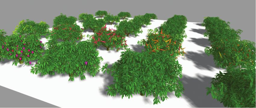
2 •      Vaillant et al.

as the appearance, growth, ageing and death of the elementary units                  To illustrate this approach, we developed a new implementa-
that are affected by physiological and environmental processes. Since            tion of V-Mango (Boudon et al. 2020), a model of mango tree
the state and the number of units change over time, simulating plant             development and fruit production that is composed of complex
growth corresponds to a class of problems formalized as dynamic                  architectural and fruit growth processes sensitive to environmen-
systems with dynamic structures (DS)2 (Giavitto and Michel 2001),                tal (temperature, light, etc.), temporal and structural factors. The
which leads to the definition of dedicated formalisms (Godin et al.              new design of the model, based on this environment, allows clear
2005) such as L-systems (Prusinkiewicz and Lindenmayer 1990).                    modularization of the original model, efficient computation,
     During the last decades, dedicated modelling platforms (Federl              easy exploration of the results and simple, reliable installation for
and Prusinkiewicz 1999; Barczi et al. 2008; Hemmerling et al. 2008;              the user.
Pradal et al. 2008; Boudon et al. 2012; de Reffye et al. 2021) have been             Our contribution can be summarized as follows:
developed. They allow the creation of a multitude of models, built

                                                                                                                                                             Downloaded from https://academic.oup.com/insilicoplants/article/4/1/diab040/6461084 by guest on 02 July 2022
on a series of specialized tools for the simulation of plant growth and             -The definition of a virtual modelling environment based on the
functioning. Such integrative platforms usually rely on software com-               Jupyter notebooks and the Python scientific ecosystem. The use of
ponents composed of multiple computer languages or formalisms.                      conda, a software environment manager, or Docker, a virtualization
Models are created as scripts or as scientific workflows (Pradal et al.             service, allows easy deployment of the environment, both locally
2008; Lang 2019). Some platforms include a visual representation of                 and remotely.
the workflows in order to give an overview of the modelled processes                -The development of wrapping and visualization tools of FSPM
and their interdependencies. However, their reuse by non-experts is                 modelling software modules for the Jupyter environment and for
usually limited to the modification of parameters, and the exploration              xarray-simlab-based scientific workflows, offering new possibilities
of model outputs (extraction, transformation, export, plotting, etc.) is            to develop models in a modular manner and simulate and visualize
often cumbersome. Extending and customizing the model generally                     plant development within notebooks.
requires inputs from the authors of the original model. Furthermore,                -The reimplementation of the V-Mango model within this
while some efforts have been made to port these tools over multiple                 environment to illustrate its use for a complex FSPM.
operating systems, reproducibility and dissemination are hampered by
the complexity inherent in their deployment and installation on new              While planning the requirements for a redesigned mango tree model
computers with different configurations.                                         and drawing conclusions from our results within a group of scientists
     On the other hand, modelling languages such as Python or R for statis-      with diverse scientific backgrounds, it became apparent that we were
tical computation propose ready-to-use ecosystems of scientific packages         addressing some issues that were relevant to a wider audience of FSPM
(Millman and Aivazis 2011). For instance, the scientific Python ecosystem        modellers and users. In particular, we addressed the shortcomings of
(Oliphant 2007) allows data processing and analysis. At the centre of these      current approaches related to dissemination, reproducibility, complex
packages, multidimensional arrays allow the user to characterize sets of enti-   model handling and interoperability, and greater genericity (Louarn
ties. Numerous tools make it possible to manipulate, visualize and perform       and Song 2020).
statistical analyses. However, these tools are generally disconnected from
FSPM simulations where flexible, graph-based structures are used to repre-                  2. T H E V I RT UA L M O D E L L I N G
sent plants. Dedicated software tools are required for parsing model input/                         ENVIRONMENT
output and extracting homogeneous views of the data for plotting or analyses.    The intent of this project is to propose a virtual software environ-
     In a new initiative to alleviate these problems, we explored the            ment that allows the creation and the execution of FSPM models. As
use of the Jupyter framework (Kluyver et al. 2016) to create virtual             reported by Capuccini et al. (2019), the idea of on-demand Web-based
modelling environments for plant models. To build the simulation                 working environments on virtual infrastructures was envisioned by
environment, we combined and extended the modules of the Python                  Candela et al. (2013). These working environments, dedicated to a
scientific ecosystems, namely numpy, pandas, SciPy (Virtanen et al.              community of practice, were originally referred to as Virtual Research
2020), xarray (Hoyer and Hamman 2017) and xarray-simlab (Bovy                    Environments. While the Jupyter project and its notebooks provide a
et al. 2021), based on multidimensional arrays to represent attributes           solid foundation for creating such environments, simulating and ana-
of plant units over time. We complemented this with the igraph library           lysing complex modelling scenarios of plant growth create specific
(Csárdi and Nepusz 2006) to build, validate and visualize the topology           needs. In particular, specific formalisms such as growth grammar need
of the plant using matrices that allow matricial algebraic operations to         to be integrated. 3D visualization and flexible interaction with 3D
model, e.g. physiological processes involving distance relationships.            shapes in a distributed way are required. Workflow formalism, possi-
Finally, we integrated the FSPM dedicated tools, L-Py (Boudon et al.             bly with a multiprocessing computation capability, to gather and run
2012) and PlantGL (Pradal et al. 2009), into the Jupyter notebooks               a set of processes that define the model, is also necessary. On the basis
and used them to efficiently model and visualize the 3D architecture             of these concepts, we propose the definition of what we call a virtual
of the plants. The key points of this environment are: (i) the seamless          modelling environment for FSPM. The different components of such
integration into Jupyter that allows the easy collaboration, dissemina-          an environment are described below.
tion, visualization and introspection of the generated data and model
processes; and (ii) a full compatibility with the Python scientific stack                    2.1 Notebook-based environment
and, therefore, direct access to the vast numpy and SciPy ecosystem              These last years have seen the emergence of a new way to communicate
since the data are almost entirely modelled as multidimensional arrays.          and collaboratively explore scientific computational ideas and data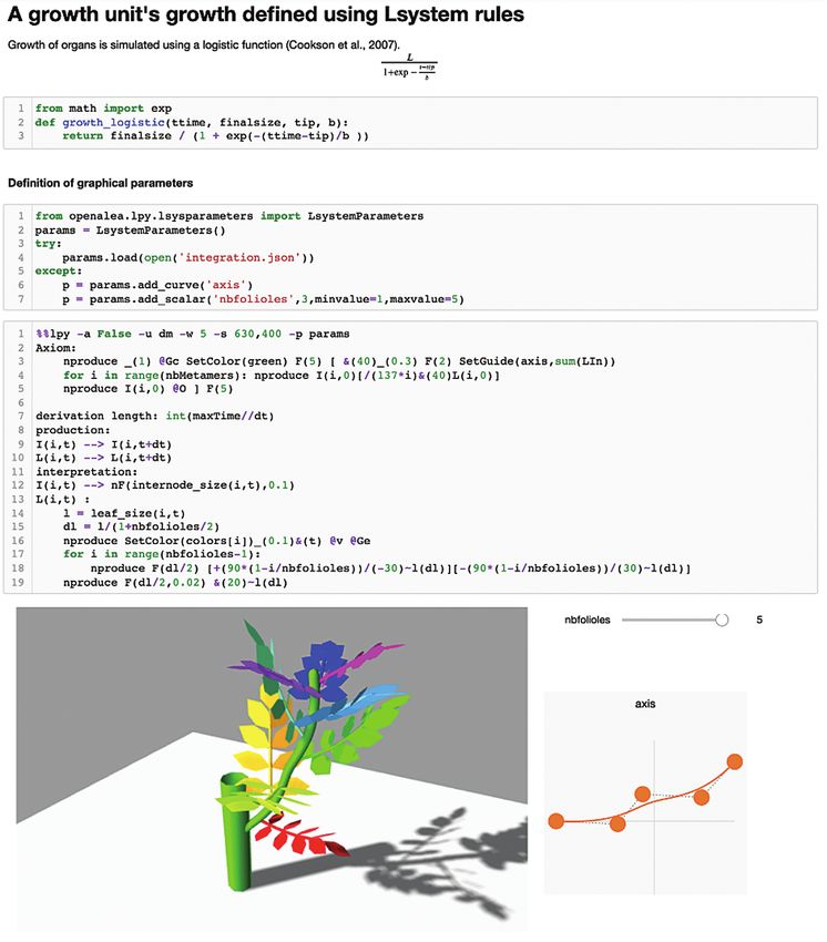
Virtual modelling environments for FSPMs based on Jupyter notebooks •           3

analysis using notebooks. In these environments, raw code is inter-         rather than the activation of a different computational kernel. Variables
spersed with charts, figures, texts and equations. This allows the crea-    are exchanged with any other Python cell. By using specific interface
tion of a shareable, interactive computational narrative (Perkel 2018)      modules such as RPy2 (https://rpy2.github.io/), L-system cells can
where analysis or modelling scenarios can be textually described, with      even be mixed with code cells from other languages such as R (see illus-
visual elements alongside their code. Some interactive features allow       tration in https://nbviewer.org/github/fredboudon/plantgl-jupyter/
the manipulation of different parts of a model and its parameters.          blob/isp2022/examples/r_and_py.ipynb).
Notebook environments emerged from the concept of literate pro-                  This L-systems integration is illustrated in Fig. 1, which rep-
gramming originally proposed by Donald Knuth (1984). They were              resents a notebook (https://nbviewer.org/github/fredboudon/
first introduced in a number of commercial analysis packages such as        plantgl-jupyter/blob/isp2022/examples/integration-demo.ipynb)
Mathematica, Maple, Matlab, and later, in open-source software such         composed of a series of cells that combine formatted text, equations
as SageMath.                                                                and both Python and L-systems code. The goal of this model is to

                                                                                                                                                        Downloaded from https://academic.oup.com/insilicoplants/article/4/1/diab040/6461084 by guest on 02 July 2022
     More recently, the Jupyter project, an open-source computational       simulate the growth of a simple growth unit. The first cell gives the
notebook ecosystem, has gained wide popularity. Part of its success         title of the notebook and mathematical details on the growth func-
is due to its clear and open format for its notebook representation.        tion. The next cell gives its Python implementation. The second cell
Moreover, thanks to a major redesign, it is possible to couple it with      of the code defines the parameters of the L-system that can be graph-
many programming languages. The foundational languages Julia,               ically controlled by the user. Using the growth function and the pre-
Python and R inspired the name of the project (Perkel 2018). Each           viously defined parameters, some L-systems rules are defined in the
language is introduced into the system as a specific computational          third cell. The cell is initiated with the magic command %%lpy, which
kernel that is responsible for the interpretation of the code (https://     makes it possible to write L-systems rules embedded in Python note-
github.com/jupyter/jupyter/wiki/Jupyter-kernels). The Jupyter pro-          books. Executing this cell directly generates a 3D dynamic plot in
ject is based on a distributed infrastructure and thus provides easy        the browser. Different buttons make it possible to navigate within the
deployment on the Internet, e.g. with the JupyterHub project. Based         simulation, allowing, e.g., the display of the entire animation of the
on this, services such as MyBinder (Auer and Landers 2019) and              simulation or forward or backward movement. Graphical parameters
Google Colaboratory (Bisong 2019) provide online services to run            appear alongside the visualization, and the simulation is automati-
any public notebook with minimal configuration. Online resources            cally updated when these values are edited. For now, parameters of
for education based on the Jupyter infrastructure have been devel-          the scalar, function and 2D curve type can be defined and manipu-
oped, like at UC Berkeley (Perez 2018), and modules such as nbgrader        lated. With such tools, it is possible to directly compare the code and
(Hamrick et al. 2017) have been developed to build online exams.            its result, interact with the model and thus provide an educational
Notebooks are also used to publish books or supplementary informa-          experience for the audience.
tion on scientific papers.
     Notebooks can be imported and run in different applications with                      2.3 The simulation framework
different styles of the Jupyter project. The standard one is the display    To organize and execute simulations, our environment is based on
of the notebook as a simple editable Web page within the browser,           the Python library xarray-simlab (Bovy et al. 2021), a feature-rich and
composed of a sequence of cells for codes and charts, figures, texts        robust extension to the xarray library.
and equations. An advanced version is the JupyterLab that makes it               The xarray-simlab library provides a framework to compose com-
possible to manage different resources and to customize the display by      plex computational models from sets of reusable components, called
arranging cell outputs in different ways so as to create a custom virtual   processes. A collection of processes can be combined to form a model,
modelling environment.                                                      and their computational ordering is entirely deduced from process
     Furthermore, dedicated Web applications can be built from note-        dependencies. In essence, those dependencies are created by explic-
books using the voila project (Voila 2020). Finally, notebooks can also     itly linking processes via output variables (producing processes) and
be displayed as interactive slideshows for educational purposes, or run     input variables (consuming processes). Variables declared within a
inside popular IDEs such as Visual Studio Code.                             process class may be annotated with other useful metadata like unit,
                                                                            description, validation functions or specific encoding settings. The
       2.2 Integrating L-systems into notebooks                             set of variables declared inside a process class describes the process
While models built with agnostic modelling languages such as Python         interface in terms of computed variables. They may be consumed by
or Java could be easily integrated within Jupyter notebooks, dedicated      any other process in the model as long as no circular dependencies
formalisms such as L-systems have been widely adopted by the mod-           are created. However, circular dependencies are allowed if a variable
elling community to create FSPMs and require specific integration.          is consumed with an offset over time, i.e. in the following simulation
As a first step to building a useful modelling environment for FSPMs,       step. For the case of interdependent variables, their evolution should
we integrated the L-systems formalism into notebooks. To do this,           be estimated within a common process, for example, using an appro-
we reused the L-Py framework (Boudon et al. 2012) that combines             priate numerical solver.
L-systems constructs with Python. Specific notebook cells can be cre-            The model—the predefined collection of processes—can be
ated with L-systems code and are executed by the L-Py interpreter.          dynamically altered by plugging in or unplugging other processes,
Since this interpreter is built on top of Python, the execution of this     or by replacing a particular process with an alternative imple-
cell corresponds to the activation of a specific mode of interpretation     mentation. Processes may inherit from a base process class, and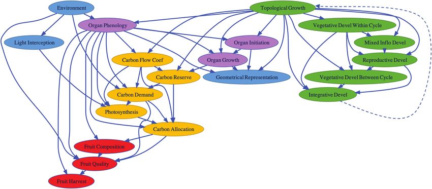
4 •    Vaillant et al.

                                                                                                                                              Downloaded from https://academic.oup.com/insilicoplants/article/4/1/diab040/6461084 by guest on 02 July 2022

Figure 1. Integration of L-systems within a notebook. Cell code that starts with %%lpy contains L-systems rules. At the execution
of the rules, a 3D visualization widget is displayed below. Graphical parameters are defined in the cell above using Python code
and displayed on the right of the 3D visualization.

derived classes may implement a different model logic and provide       In order to execute a particular model, users create a model set-up
additional output variables. Models and their processes and vari-   in which they define the basic parameters for each simulation run. The
ables can be programmatically inspected, and the computational      most important are the time steps, the values of the model input vari-
order, i.e. process dependency, can be easily visualized.           ables and the name of the variables to be exported.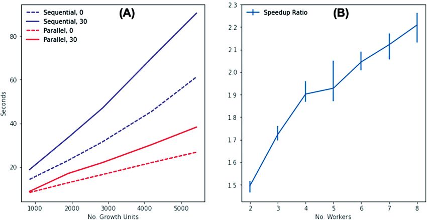
Virtual modelling environments for FSPMs based on Jupyter notebooks •             5

    The xarray-simlab library provides great freedom in the design of              multidimensional arrays (in general, from the numpy library)
a model and numerous ways to declare variables. We decided to sepa-                and provides tools to analyse and plot such arrays. Using such
rate three types of numerical data: pure constants like natural physi-             tools for items stored within flexible structures requires the
cal constants that are kept directly inside a Python module, variables             definition of queries to parse the structures and extract values in
that effectively vary during a simulation, and parameters that are either          an appropriate order.
obtained from the literature or after a calibration process and are there-    (ii) A lack of control over data consistency. Loosely typed data
fore constant within a simulation set-up. Each individual process may              structures such as MTG do not ensure that values for a property
be parameterized with these separate files stored in the toml format.              stored within a tree are of identical types. Type checking needs
By default, an initialization function is associated with each process             to be introduced to ensure compatibility with standard scientific
to load those parameter files and parameterize a process at startup.               stacks.
However, it is still possible to inject custom parameter values by reim-     (iii) Difficulties to store time series data, which are typical for

                                                                                                                                                           Downloaded from https://academic.oup.com/insilicoplants/article/4/1/diab040/6461084 by guest on 02 July 2022
plementing a process initialization function.                                      most biological process models. By default, the standard plant
    Simulation inputs and outputs are mostly composed of xarray data               data structures for FSPM are mainly designed to represent
structures (i.e. labelled arrays and data sets). All features from xarray          the current state of the simulation. Time series of structures
are therefore readily available for all input and output data: index- and          can be created, but mapping between entities over time is
label-based selections; interpolation and grouping of data; reshap-                challenging. Alternatively, time series of property values can
ing and combining data sets; reading and writing files; and advanced               be directly stored within a structure. However, trees need to
plotting.                                                                          be parsed each time one wants to export the time series of the
    To adapt this framework to FSPMs, we have extended the                         properties of different structure entities in order to manipulate,
library with new features. L-systems models can be automatically                   analyse or plot them.
integrated as processes, and the simulation runs with associated             (iv) Possible computational inefficacy if operations need to be
visualization (see following Section 2.4 below). While FSPMs                       repeatedly applied on every or on a large subset of entities.
simulate structures with a growing number of elements, xarray-                     In particular, structure parsing and type checking creates a
simlab is originally designed to model the dynamics of structures                  performance overhead that can be avoided when working
with a fixed number of elements. We extended it so that all prop-                  directly with multidimensional arrays. Moreover, array-based
erty arrays are automatically and consistently resized when new                    operations, optimized at the C level, generally outperform
entities are created. The growth of the entity index over time does                equivalent operations built using pure Python.
not make it possible to use xarray-simlab built-in parallelism capa-
                                                                             We therefore explored ways of expressing the properties of plant mod-
bilities. We therefore reimplemented the parallel processing of
                                                                             els and their topologies in multidimensional arrays by essentially creat-
multi-model simulations using Python’s standard multiprocessing
                                                                             ing arrays for properties and an adjacency matrix (a standard matrix
library. Our solution is not as efficient as some GPU-based solu-
                                                                             representation of graphs). An additional time dimension may also be
tions for L-systems (Lipp et al. 2010), but it offers great flexibility
                                                                             required for all properties that vary over time. A data structure, referred
and expressiveness to define modelling processes thanks to Python
                                                                             to as a data set, from the xarray library makes it possible to assemble
and its scientific ecosystem.
                                                                             the different properties and the topology in a coherent way. A con-
                                                                             straint is that all entities have a common set of properties for their rep-
                   2.4 Plant representation                                  resentation. L-system string representations are made compatible with
Plants can be seen as a collection of entities of various natures (e.g.      the data set of properties by associating a unique id with each module
vegetative and reproductive units). The topological relationship of          of the L-systems string that represents the position in the arrays of the
those entities can be expressed as a tree graph, possibly multiscale         properties of the entities.
(Godin and Caraglio 1998). Dedicated data structures such as the                 The main challenge is to take the growing number of entities over
multiscale tree graph (MTG) (Pradal and Godin 2020) or a brack-              the simulation time into account. To do this, we extended the xar-
eted string representation (Prusinkiewicz and Lindenmayer 1990)              ray-simlab framework to provide an automatic extension of the data
have been developed to represent and manipulate these structures.            structure representing the plant. Every array representing properties
Those representations have various advantages, like easy traversals          or topology is extended with new default values upon the appearance
through the parent–child relationships and the possibility to store          of new entities. By default, the NaN value is used to express the fact
items with arbitrary structures and properties of various types              that a value is not set (i.e. entities that have not yet appeared or have
within the tree.                                                             been pruned) and should be determined by the appropriate process.
    However, this flexibility comes with a cost and has several disad-       As a constraint, the values are all expressed as floating-point values (the
vantages that may make it a suboptimal choice, depending on the spe-         only nullable data type available).
cific model structure, the research question and the requirements of
the model environment. The main disadvantages are:
                                                                                  2.5 Integrating L-systems into the simulation
  (i) No straightforward transformation to and from array structures                                workflow
      suitable for utilizing features of the standard Python scientific      The definition of the processes of a simulation workflow based on
      stack. By default, the Python scientific stack is based on             xarray-simlab requires the precise definition of input and output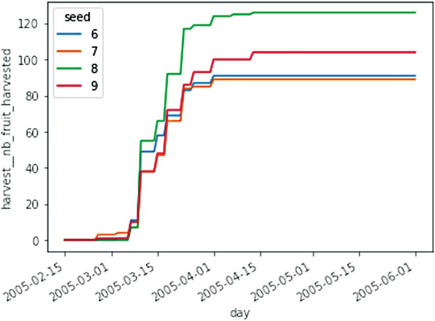
6 • Vaillant et al.
variables, and an execution function for each process. In the spe- the L-system code, automatically exposing in and out variables. For
cific case of L-systems, input and output variables can be directly the out variables, the lpyprocess function individually exports
deduced from the model definition. Using L-Py specifications, all the parameters of the custom modules as arrays. For instance, the
model input variables are defined using the extern command. Metamer_t variable stores all values for parameter t of all Metamer
These variables are directly exported onto the process interface. modules. Although it is transparent from the L-system point of view,
As output, an L-system generates topological structures in the the redirection of the module parameters into arrays is made through
shape of L-strings, and 3D representations. To be compliant with specific Param structures that are automatically generated for the
the array-based plant representation of the simulation frame- simulation. For each module of an L-string, the Param structure
work, the parameters of the different modules of the L-strings are mainly stores the id of the module it represents and has the possibility
grouped and stored as individual arrays. For each type of module, of retrieving or modifying its associated parameters within the array
an index array is also generated. This makes it possible to directly representation.
Downloaded from https://academic.oup.com/insilicoplants/article/4/1/diab040/6461084 by guest on 02 July 2022
access and manipulate all values of the parameters of all entities of The third cell of the code defines a second process that
the same type. simulates a simple carbon allocation procedure. To do this,
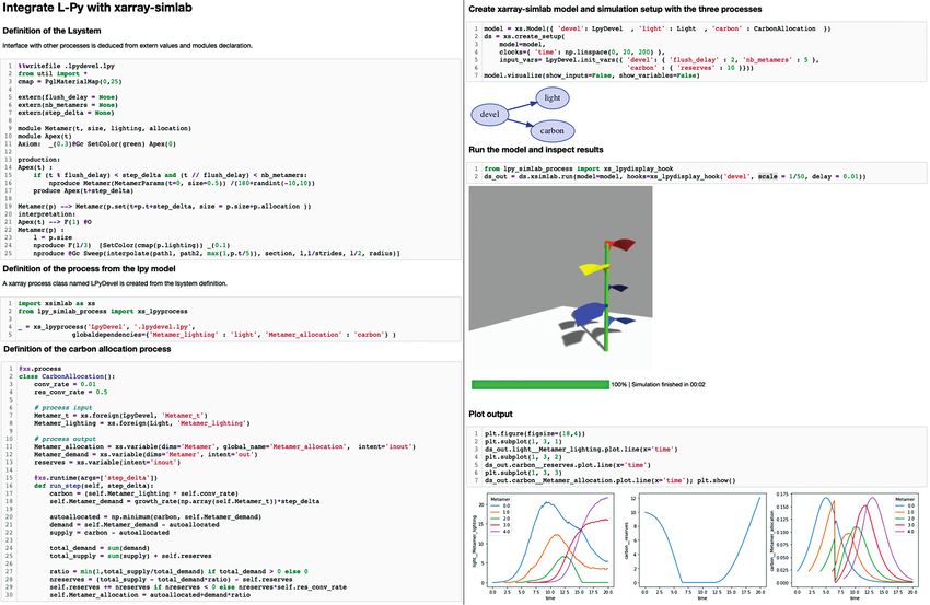
The integration of L-systems within the xarray-simlab scien- some parameters of the L-system simulation are used, such as
tific workflow is illustrated in Fig. 2 (https://nbviewer.org/github/ Metamer_t. Other parameters are filled in by the process,
fredboudon/plantgl-jupyter/blob/isp2022/examples/lpy-simlab/ such as Metamer_allocation. Another process (code not
lpy_carbon_light.ipynb). In the first cell, the code of an L-system is shown) simulates the intercepted light (from a zenithal light
defined. The extern commands (lines 5–7) define the input vari- source in this example). The fourth cell assembles these pro-
ables that control the simulation. Note that the step_delta is a cesses into a simulation workflow, defines its set-up and visual-
custom variable of xarray-simlab that gives the current step duration, izes it. The workflow is then run and some of the variables are
which is required as input for each step of the L-system simulation. explored and visualized as 2D plots, such as the amount of inter-
The second cell of the code generates an xarray-simlab process from cepted light per metamer over time.
Figure 2. Integration of L-systems within a notebook-based scientific workflow.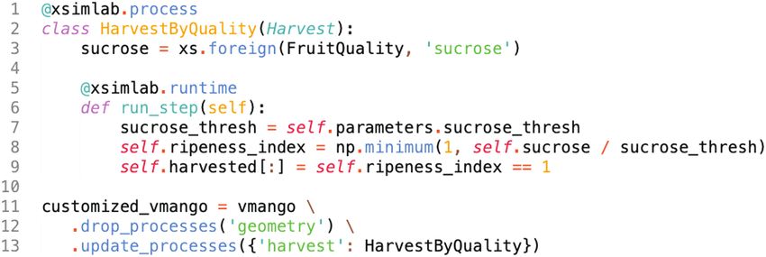
Virtual modelling environments for FSPMs based on Jupyter notebooks •             7

             2.6 3D visualization of plants in a                             PlantGL could be made readily available in JavaScript. Nevertheless,
                   client-server context                                     minimal computational capabilities are required for the client. Our
Both execution of the model and visualization of the simulation results      approach might be suboptimal for less well-equipped terminals such
are performed inside Jupyter notebooks using the plantgl-jupyter             as tablets or smartphones.
module (Vaillant and Boudon 2021). The Jupyter framework has a
distributed architecture with a client (Web browser) and a server that             2.7 Deployment of the virtual environment
contains the actual execution of the model. The result of a simulation       In order to deliver deployable software modules for reproducible sci-
must therefore be communicated by the server to the client using             ence, we rely on the conda management system. It allows us to build
Internet protocols and be rendered by the Web client. While stand-           a software environment relatively independent of the host operating
ard protocols for streaming and display of pictures and 2D charts have       system. An environment is simply specified using a text file that lists all
been adopted for a long time, the case of the 3D representation is less      the required software modules and, possibly, their version. An environ-

                                                                                                                                                           Downloaded from https://academic.oup.com/insilicoplants/article/4/1/diab040/6461084 by guest on 02 July 2022
clear. Different libraries allow the definition and the streaming of 3D      ment can be created locally or on online services such as binder from
shapes (pythreejs, k3d, etc.). From the client side, high-level JavaScript   this file.
libraries such as three.js (mrdoob 2021) allow the rendering of 3D               To create custom FSPM environments, some of the software mod-
shapes in the browser using WebGL.                                           ules we developed, such as PlantGL and L-Py, were packaged for conda
    To have interactive visualization, the time necessary to transmit the    so as to be easily deployed. To rapidly build and assemble these pack-
3D representation has to be minimized. This time can be broken down          ages, we defined a releasing pipeline based on online services for open
into a time to encode the representation into a streamable representa-       software. Code is managed on the GitHub repository that is now con-
tion, the actual time of streaming and the time to decode the represen-      figured to trigger automatic build on continuous integration services
tation, convert it into three.js objects, and the time for the rendering     such as GitHub Actions or AppVeyor. If the build is successful and
itself. Streaming time is proportional to the size of the encoded data,      passes the automatic tests, a new version of the package is automati-
while encoding and decoding are proportional to the size of the origi-       cally published on the conda package online database (https://ana-
nal 3D scene. We tested different procedures to serialize and stream         conda.org/), currently in the fredboudon channel. This allows the
3D representations with minimal encoding and streaming time, and             rapid publication of new features and bug correction, while preserving
we evaluated their benefits.                                                 previous versions for reproducibility of previous environments.
    We first tested the pythreejs library (https://pythreejs.readthe-
docs.io/) that wraps three.js in Python and allows the streaming and                        3. A P P L I C AT I O N TO T H E
display of 3D objects in a Web browser. The advantage of such an                                V- M A N G O M O D E L
approach is that a similar representation is used both by the server and     The integrative FSPM V-Mango was recently developed to simu-
the client, minimizing data transformation. However, it does not allow       late mango tree growth, phenology and fruit production (Boudon
a straightforward high-level representation for plants, and it leaves        et al. 2020). Mango is an important fruit from tropical and subtropi-
too little room for customizations. As such, many objects need to be         cal regions and its cultivation faces several agronomic challenges. In
stored with low-level mesh representation. Furthermore, due to its           particular, it exhibits (i) phenological asynchronisms partly due to
architecture, every custom user interaction with the browser’s canvas        complex interactions between vegetative and reproductive growth
(where the 3D scene is rendered) must be transmitted to the server’s         (Dambreville et al. 2013; Normand and Lauri 2018), and (ii) fruit
Python runtime, which in turn issues a signal to the renderer. This pro-     heterogeneity at harvest in terms of size, gustatory quality and post-
cess slows down the visualization and user interaction. As an alterna-       harvest behaviour. To understand such a complex behaviour, the
tive, we tested the Draco mesh compression library (https://google.          precise modelling of the development of the mango tree architecture
github.io/draco) that proposes an efficient compression algorithm that       and its constituents (growth units (GUs), inflorescences and fruits)
makes it possible to minimize streaming time. The drawback is that it        was required. A number of developmental processes were formalized
requires converting the entire 3D representation into a single mesh,         and assembled. In the first version of the model, these processes were
thus removing semantic information contained in the 3D scene.                implemented as simple functions or L-system rules with no way to dis-
    Finally, we tested an alternative method that consists in directly       tinguish them from each other, except by their names. The model was
using the serialization methods for 3D objects of the PlantGL library        implemented using Python, R and the L-Py framework. Glue-code
(Pradal et al. 2009) and combining it with a standard zip compression        between these different technologies was based on code developed
format. PlantGL representation allows the use of massive instantiation       in-house. In particular, the fruit model was implemented in R and,
and high-level primitives with compact representation. From the client       because of the simple interface provided, no interaction with the other
perspective, a port of the PlantGL API can be created using its original     submodels written in Python was possible.
C++ code and a WebAssembly transpiler such as Emscripten (Zakai                  In the new version of the model, called vmango-lab and published
2011). With such an approach, server and client share a high-level geo-      at https://github.com/fredboudon/vmango-lab/tree/isp2022 under
metric representation. Discretization of the geometry for rendering is       an open-source license, we used the virtual modelling environment
made by the client, allowing the server to dedicate its computational        based on the notebooks presented above to redesign the model and
capability to the simulation. This last approach proved to be efficient      reorganize its code. Most of the work consisted in defining processes
with minimal coding costs since C++ routines already implemented in          and their inputs/outputs, and assigning corresponding model logic.
8 • Vaillant et al.
Code was also adapted to the use of multidimensional arrays to store generalized linear models, and probabilities were determined by archi-
parameter values. This new modular implementation allows the cus- tectural and temporal factors (Dambreville et al. 2013; Boudon et al.
tomization of the model for new use cases. To illustrate this, we pre- 2020). Different automata were formalized for the different types of
sent in the following sections the application of vmango-lab for testing entities (GUs, pure inflorescences and mixed inflorescences). For veg-
carbon allocation strategies at the scale of individual GUs, and for etative development, GUs appearing during the same growing cycle
performing parallel multi-model simulations. For each of the cases as their mother GU are distinguished from the ones appearing dur-
presented, a notebook with further detail is available at https://github. ing the following cycle since different factors affect their appearance.
com/fredboudon/vmango-lab-demo/tree/isp2022. All of this developmental information is contained in the Integrative
Developmental process that updates the developmental attributes.
3.1 Modularity and redesign of the V-Mango Finally, the Topological Growth process uses this developmental infor-
processes mation to extend the plant representation at each time step according
Downloaded from https://academic.oup.com/insilicoplants/article/4/1/diab040/6461084 by guest on 02 July 2022
V-Mango is a complex model where different processes simulate the to the simulated appearance date (feedback represented with a dashed
growth and the phenology of the mango tree and its constituents of arrow on the diagram).
interest (GUs, inflorescences and fruits). To have a homogeneous and A second set of processes, represented in purple in Fig. 3, simu-
simple representation, the model formalizes the tree as a collection of lates the development and growth of the individual entities. To do
GUs with flowering and fruiting attributes to represent information on this, potential growth is estimated from empirical distribution (Organ
inflorescences and fruits. During the simulation, the variables repre- Initiation process), thermal time models are run for the development
senting the different attributes of the GUs are passed between the dif- and the growth of each entity (Organ Phenology process) and their
ferent processes of the model and their values are updated to simulate spatial dimensions are increased accordingly (Organ Growth process).
the development of the mango tree and its constituents of interest. The The specific case of fruit growth in terms of dry matter is modelled
model is now formalized as the sets of processes depicted in Fig. 3. based on carbon exchange. To do this, we extended and modular-
A first collection of processes, depicted in green in Fig. 3, simulates ized the carbon balance model proposed by Léchaudel et al. (2005)
the appearance of the botanical entities in the architecture at differ- for mango fruiting branches (represented in yellow in Fig. 3). First,
ent time steps. The appearance of these entities is broken down into carbon supplies (reserves and assimilation by photosynthesis) and
elementary stochastic events that describe the occurrence, the inten- demands (maintenance and growth) are estimated by different pro-
sity and the timing of their appearance and are modelled by binomial, cesses. Carbon reserves are estimated for the different GUs as a func-
Poisson and ordinal multinomial distributions, respectively. These tion of their size (Carbon Reserve process). Carbon demand for organ
distributions are assembled into a stochastic automaton that simulates maintenance and fruit growth are determined in the Carbon Demand
the number, timing and fate (purely vegetative, flowering or fruiting) process as a function of organ size and potential growth for each fruit.
of new entities appearing on each terminal GU. The different distri- Carbon assimilated by photosynthesis (Photosynthesis process) is cal-
butions were parameterized from measured architectural data using culated from intercepted light given by the Light Interception process.
Figure 3. Workflow of the new V-Mango model. The diagram has been directly generated from the code, except for the dashed
arrow. Explicit names to explain process purposes are used. Abbreviated names for processes are also used in the code (see
Supporting Information—Table S1 for correspondences).Virtual modelling environments for FSPMs based on Jupyter notebooks • 9
At this time, light interception is chosen from microclimate environ- 3.3 Customization of the modelling workflow
ments measured within canopies.
Based on the estimations of carbon supplies and demands, and Thanks to the introduced modularization, alternative processes can
on the exchange parameters determined from distances between be easily defined to replace predefined ones. In the following example,
GUs (Carbon Flow Coef process) and allocation rules, the Carbon changes in the Fruit Harvest process are illustrated in Listing 1. A new
Allocation process performs the allocation of carbon between organs process to test the sucrose content of the fruit is defined. This process
and functions. Priority for carbon allocation is as follows: organ main- is defined as a Python class with the @xsimlab.process deco-
tenance is first satisfied with local carbon supply; supplementary rator (lines 1–2). Its run_step function (lines 4–8) first retrieves
carbon is then exported to demanding fruiting GUs according to the the variable sucrose that represents the sucrose content of each
estimated distance-based flow coefficient; and finally, fruit growth in fruit with an array. The ripeness index is set to 1 if the sucrose con-
dry mass is determined from their allocated carbon. tent exceeds the threshold sucrose_thresh defined as a param-
eter of this process. A new model customized_vmango is then
Downloaded from https://academic.oup.com/insilicoplants/article/4/1/diab040/6461084 by guest on 02 July 2022
A last set of processes, represented in red in Fig. 3, simulates fruit
growth in fresh matter and fruit quality. We integrated the model pro- instantiated (line 11) as a copy of the vmango model, with removal
posed by Léchaudel et al. (2007) for mango fruiting branches. The of the geometry process (that computes the geometrical represen-
amount of soluble sugars, starch, acids and minerals in the fruit is tation). The harvest process is replaced by the new custom process
empirically linked to fruit age and fruit dry mass (Fruit Composition HarvestByQuality. This non-visual, and thus faster, model
process). Fruit growth in fresh matter is then modelled by water- makes it possible to test for an alternative harvesting policy.
related processes (water inflow into the fruit, driven by stem and fruit
water potentials, and fruit transpiration), and sugar content is calcu-
lated (Fruit Quality process). The Fruit Harvest process calculates a
ripeness index for each fruit. By default, the index is estimated as a
threshold on the thermal time sum of the fruit.
3.2 Estimating carbon fluxes from a distance matrix
In the original model, carbon demand (for GU maintenance and
fruit growth) and supply (from reserves and photosynthesis) were Listing 1. Customizing a model by replacing a process and
globally estimated for all the GUs composing a fruiting branch. As a unplugging another one (code slightly simplified for clarity).
limit, no topological change in the structure was allowed during fruit New modelling workflows can thus be designed by partly reusing the
growth. In order to model more detailed exchanges, all GUs are now default workflows. For instance, in the notebooks https://nbviewer.org/
considered separately. Their carbon exchanges with the surrounding github/fredboudon/vmango-lab-demo/blob/isp2022/notebooks/1-
fruits are explicitly formalized using an exchange matrix (Carbon 0-modularity.ipynb and https://nbviewer.org/github/fredboudon/
Flow Coef process) based on distances that can be re-evaluated at vmango-lab-demo/blob/isp2022/notebooks/1-1-arch_dev.ipynb, a
the appearance of each new GU. The distance between two GUs is workflow focussing on the architectural development alone is designed.
expressed as the number of GUs in the shortest path between the In contrast, in https://nbviewer.org/github/fredboudon/vmango-lab-
two GUs in the tree structure. To reproduce the assessment of the demo/blob/isp2022/notebooks/4-use_case_measure_and_simulate.
level of carbon autonomy of branches according to their size found ipynb, presented in more detail in the Section 3.5, a fixed architecture is
in the original version of the model, only carbon flows between GUs considered and only phenology and fruit growth are simulated. A variety
at a distance d from a fruit below a given threshold dmax are consid- of workflows can thus be designed according to the modelling needs.
ered. The carbon flow coefficient Fij from a leafy GU i towards a fruit Since workflows are coupled with L-systems, it can also be seen as a way
borne by GU j, with GU j belonging to the set J of fruiting GUs, is to introduce modularity within L-system models.
calculated as:
3.4 Distributed simulations and visualization
H(dmax − dij ) The performance of the modelling environment and of the visu-
Fij = ∑J
(1) j H(dmax − dij ) alization tools is important to provide the user with an interactive
and intuitive experience of the modelling process. The techno-
where H represents the heaviside step function equal to one when logical stack presented in this manuscript already provides many
distance d is less than or equal to dmax, and zero otherwise. This func- excellent solutions to overcome these challenges. However, cer-
tion can be seen as a simplified version of the distance-based allocation tain aspects of our particular model logic and data representa-
function proposed in previous studies (Lescourret et al. 2011; Reyes tion, such as the inherent dynamic nature of the topology and
et al. 2020). The distance between all GUs in the structure is efficiently the rendering of its geometric representation, required solutions
computed using SciPy routines and, in particular, the ‘shortest_ that were not readily available. These solutions had to be imple-
path’ function, from the adjacency matrix representing the tree mented, in particular, the visualization of large PlantGL scenes
structure. The distance matrix makes it possible to test more complex in a notebook context and multi-model parallelization. To evalu-
carbon allocation scenarios in the future. ate the usability and interactivity of the proposed visualization10 • Vaillant et al.
system, we first assessed its performance on complex mango Listing 2 : Creating and running a set-up in batch (parallel)
models. In a second step, we assessed the possibility to launch, mode and plotting of results.
display and analyse in parallel simulations with different initial The batch option (line 2) of the vmango-lab run function made it pos-
conditions. In the model development process, these features sible to pass the array of parameters used by the parallel execution. The
offer interesting possibilities for calibrating a model or running a 3D view of the parallel simulations was updated by each simulation
sensitivity analysis more efficiently. independently, allowing a pleasant interactive view of the develop-
On the basis of our tests, the rendering engine was able to effi- ment and fruit production of the virtual ‘orchard’. Results of the dif-
ciently transmit and render large scenes with great detail, even ferent executions were assembled into a common data set and could
if the scene was generated on a distant system (Fig. 4). Our test be directly plotted (line 4), resulting in the diagram shown in Fig. 5.
machine was a laptop with a Debian GNU/Linux 10 system with The performance of a simulation run varied with the size of the ini-
16 GB of memory and an Intel® Core™ i5-8250U CPU @1.60 tial tree, the number of time steps, the number of geometries derived
Downloaded from https://academic.oup.com/insilicoplants/article/4/1/diab040/6461084 by guest on 02 July 2022
GHz × 8, Intel® UHD Graphics 620. With the model execution during the simulation and, last but not least, with the number and fre-
and the visualization in the Web browser distributed locally, the quency of model outputs that needed to be merged into the resulting
transmission took several milliseconds. The frame rate (FPS) of xarray data set. As a test case, we benchmarked the duration of a simu-
the display varied from 40 to 10 for an average tree with 2000 to lation run, both in sequential (four model runs on a single CPU core)
3000 GUs (approximately 107 triangles), depending on the num- and in parallel mode (four model runs, each on a single CPU core),
ber and level of details in associated GU organs like leaves, flow- over 2 years (daily time steps) with a varying number of GUs in the
ers and fruits. Similarly, large scenes representing orchards (Fig. 4 initial tree, and generating 3D visualization every 30 steps or only at
and Supporting Information—Video 1) were smoothly visual- the end of the simulation. The model was initialized with trees com-
ized, and user interactions like rotation and zoom were seamlessly posed of 100–500 GUs. At the end of the simulation, final trees had
performed. 800–5500 GUs, which roughly translated into 4- to 10-year-old mango
In a second test, a synthetic mango orchard [see Supporting trees. The total simulation time increased linearly with the number of
Information—Video 1] was simulated. Each mango tree was initial- GUs of the final trees, with a higher slope for sequential simulation
ized with the same structure, but different seed values controlled the and 3D visualization generated every 30 steps (Fig. 6A). A compari-
random number generation used during the stochastic processes of son between sequential and parallel simulation shows an increasing
tree development (Fig. 4). speedup ratio with the number of cores used, and ranging from 1.5 to
Depending on the number of available CPU cores, multiple simula- 2.2 for 2–8 CPU cores (Fig. 6B). The general performance was reason-
tions were run in parallel with only a few lines of code (Listing 2 able for a typical simulation set-up run on a personal computer.
However, for very large trees with several thousand GUs, the
factor limiting computational time could be the available com-
puter memory rather than the number of cores or the capacity of
.) CPUs and GPUs. Since square adjacency and distance matrices
Figure 4. 3D rendering of a tree at selected simulation steps during several successive growing cycles. Simulation steps are from
leftmost in the back to rightmost in the front.Virtual modelling environments for FSPMs based on Jupyter notebooks • 11
grow exponentially with the number of GUs in the tree, the mem- 3.5 Study case: investigating source–sink relation-
ory required to hold the data grows likewise. For example, allocat- ships on measured architecture
ing a single full distance matrix for a tree composed of 20 000 GUs The vmango-lab allows a wide range of uses and applications in
requires 1.6 GB of memory (float32 data type). In the future, this agronomical research. In this section, we illustrate how the model
limitation could be alleviated by integrating sparse implementations could be used to investigate source–sink relationships, a widely
of multidimensional arrays in xarray-simlab based, for example, on studied issue in fruit production, by manipulating the Carbon
a representation defined in the sparse library (https://sparse.pydata. Allocation process through the threshold distance dmax (Equation
org). Alternatively, a vmango-lab environment can be deployed on a (1)). Model modularity makes it possible to run simulations for
virtual machine with a configurable amount of memory if required fruit growth- and fruit quality-related processes (represented in
for large simulations. yellow and red, respectively, in Fig. 3), using observed architecture
instead of architecture simulated with architecture-related pro-
Downloaded from https://academic.oup.com/insilicoplants/article/4/1/diab040/6461084 by guest on 02 July 2022
cesses (represented in green in Fig. 3). The corresponding note-
book can be found at https://nbviewer.org/github/fredboudon/
vmango-lab-demo/blob/isp2022/notebooks/4-use_case_meas-
ure_and_simulate.ipynb.
The study case consisted in a girdled branch bearing one fruit,
whose architecture (topology, stem diameter, stem length and leaf
number of all GUs) was measured in the field and represented with
a simple drawing (Fig. 7A1 and A2). These data were easily formatted
into a csv file used as model input. A 3D (mock-up, Fig. 7B) and a 2D
(igraph, Fig. 7C1) representations of the observed architectural data
set were generated by the model. Carbon flow between a GU and a
fruit is controlled by a distance-based allocation function (Equation
(1)). It was assumed that only leafy GUs, i.e. those producing pho-
toassimilates, located below a threshold distance dmax to a fruit allocate
carbon to support the growth of this fruit. Carbon flow from a leafy
GU i to the fruit borne by GU j is proportional to the carbon flow coef-
ficient Fij that depends on the distance dij (Equation (1)). The set of
Figure 5. Cumulated number of fruits harvested per tree, leafy GUs supporting fruit growth according to dmax is illustrated in Fig.
plotted from the resulting data set of a parallel batch run of four 7C1 using an igraph representation of the data, for dmax values of 4 or
simulations (four trees) with different seed values. 10 GUs. Fruit growth in fresh mass was simulated in these two cases,
Figure 6. Evaluation of simulation performances. (A) Comparison of computational time (seconds) of four simulation scenarios:
two parallel multiprocessing simulations with four models run on four cores (in red) and two sequential single process (in blue)
simulations of four model runs, both with either a geometry derived at the end of the simulation (0) or a geometry processed
every 30 days (30); (B) Speedup ratio: time elapsed for n models in a sequential, single process simulation over time elapsed for n
workers (cores/processes) in parallel mode with 10 repetitions (mean, minimum and maximum values are displayed).12 • Vaillant et al.
and predicted and observed fruit fresh mass at harvest were com- 4. D I S C U S S I O N
pared (Fig. 7C2). The light environment was set to an average default 4.1 Notebooks for FSPM
value for all the GUs of the branch. However, it would be possible to The Jupyter-based modelling environment presented in this manu-
use observed values if the light environment was measured. Results script brings together and customizes scientific and modelling tools of
showed that 10 GUs was certainly a more adequate dmax value than 4 the Python ecosystem to build robust and shareable FSPMs. Building
GUs, indicating that almost all the leafy GUs of the branch might have on such an environment makes it possible to benefit from the regular
contributed to fruit growth. By varying the value of the input param- improvements of this dynamic ecosystem. At the centre of the Jupyter
eter dmax, it is possible to explore different source–sink relationships project, the notebook format allows the user to create a computational
within the branch through simulation. The approach developed at a narrative of a modelling scenario. Such an approach is efficient because
local (branch) scale could further be extended at a global (tree) scale, it allows collaborators and users to test a model, as illustrated by the
as proposed, for example, in peach (Lescourret et al. 2011) or apple notebooks that supplement this manuscript, thus demonstrating the
Downloaded from https://academic.oup.com/insilicoplants/article/4/1/diab040/6461084 by guest on 02 July 2022
(Pallas et al. 2016) fruit crops. reproducibility and ease of dissemination of research work on FSPMs. In
Figure 7. Protocol of use of the fruit model on measured architecture. (A) Data acquisition in the field: (A1) picture of the original
branch; and (A2) drawing of the manual measurement of the branch architecture. (B) Reconstruction and 3D visualization of the
branch (a fake trunk was added for visualization). (C) Fruit growth simulation with a threshold distance (dmax) of 4 and 10 GUs
for the Carbon Allocation process, and visualization of model outputs: (C1) carbon flow between all GUs and the fruiting GU;
and (C2) simulated fruit fresh mass dynamics as of the end of fruit cell division (time = 0 d). Red numbers in pictures A1, A2 and
B and numbers in picture C1 are the GUs’ id. Orange, green and white dots in picture C1 represent the fruiting GU, leafy GUs
and GUs without leaves, respectively. Red arrows represent the distance between source and sink GUs, with arrow width inversely
proportional to distance. The red point in picture C2 is the observed fresh mass of the fruit at harvest.Virtual modelling environments for FSPMs based on Jupyter notebooks • 13
particular, the use of notebooks and the conda package management sys- The possibility of distributing simulation computation allows the
tem make it possible to clearly specify software dependencies, hypoth- efficient computation of multiple models with varying parameters,
eses of the model and actual parameter values. There is still a possible and thus makes it possible to perform efficient sensitivity analysis. As
limitation since the link to any external sources of data can be inconsist- it comes natively within our framework, this feature is easy to use. As
ent over time and create non-reproducible experiments. A solution to a future step, modelling the growth in parallel of a multitude of plants
this problem is to reference only the data distributed in the modelling would create interesting possibilities for the study of crop growth.
project or to follow the FAIR guidelines (Wilkinson et al. 2016). However, this would make it necessary to account for plant interac-
Moreover, organizing the code, the descriptive texts and illustra- tions, and to thus extend the modelling formalism to allow interactions
tions in a didactic way requires special care. The notebook cells can between processes computed in parallel.
be executed in any order. This has the advantage of allowing flexible The virtual modelling environment presented in this manuscript
experiments, but makes it sometimes difficult to assess the exact origin is largely based on Python. Some modelling softwares of the FSPM
Downloaded from https://academic.oup.com/insilicoplants/article/4/1/diab040/6461084 by guest on 02 July 2022
of the results. As such, notebook design policy should be followed to community are built using alternative programming languages such as
ensure consistency of the experiments over time (Rule et al. 2019). C++ or Java (Hemmerling et al. 2008; Griffon and de Coligny 2014).
Jupyter notebooks are compatible with a large number of languages,
4.2 Continuous delivery including Java and C++. Communication between languages is facili-
Relying on the conda management system to access standard scientific tated by the Jupyter project but can still be complicated in some cases
tools and to package some of our specific modelling tools proves to be (e.g. Python-Java). As a result, integrating Java-based tools within the
efficient and allows easy deployment over different computers with dif- framework presented here would be difficult. However, similarly to
ferent operating systems or clusters or clouds. The continuous delivery what we did with Python, L-Py and PlantGL, integration of Java-based
pipeline we used, based on online services, allows us to develop new FSPM modules into Jupyter can certainly be undertaken in order
features more transparently for collaborators and users since they can to provide a complementary Java-based modelling environment in
have a view of the new code produced and its releasing state through notebooks.
the pipeline. Based on our experience, this fosters the interaction with
other groups and the diffusion of the software. 4.4 Collaborative design of workflows
Rather than maintaining ‘second-order’ documents about processes,
4.3 FSPM modelling dependencies, variables and units, we looked for an approach that
The adaptation of Jupyter notebooks to FSPMs requires the integration would enable us to directly inspect the model code—as the single
of specific tools and formalisms such as L-system and 3D visualization source of truth—and to visualize the model structure in order to col-
capabilities. The possibility to mix cells of L-system code with standard laboratively develop the model and its processes without the need to
code and detailed descriptions containing text, equations and figures inspect the actual source code itself. Due to the model modularity and
makes it possible to create a modelling narrative, with different cells the choice of process granularity, the model can be easily extended and
to compute, display and comment on the different results of the nar- adjusted, even by collaborators with moderate proficiency in the pro-
rative. Nevertheless, the L-system code has a non-standard execution gramming language. This increases the usability of the model and its
mode since it generates an entire animation. The visualization inter- environment for a larger group of researchers.
face allows the exploration of this animation by running the model as With such features provided by xarray-simlab and our customiza-
a whole or for a reduced number of steps. Several modes of execution tions, vmango-lab allows fast model development, interactive model
are thus nested in such a notebook: the execution of the L-system cells exploration and collaborative model design—not least due to its seam-
and the execution of the steps of the model. This may be particularly less integration into the Jupyter framework. However, if required, any
confusing for the beginner. Our experience revealed that computer simulation and model can be run headless (without a Jupyter frontend
science Master’s students were at ease with such an approach, while or kernel) as a standard Python module. This is particularly important
plant science Master’s students with little programming experience for efficient debugging.
preferred the standard L-system interface provided by L-Py. One rea-
son for that was the limited debugging tools provided by the notebook 4.5 Data representation
environment, in particular, for the execution of an L-system model. In Many aspects of xarray and xarray-simlab have been designed for
order to improve the tools, it would therefore be important to upgrade use in the earth sciences and thus have a strong focus on longitude–
this feature. latitude grids. These libraries therefore have no generic support for
The 3D visualization of the growth of a plant structure mod- modelling topological relations and graphs such as plant entities.
elled with an L-system requires an interactive visualization. The In particular, they lack support for growing structures (i.e. grow-
existing solutions were considered to be unsatisfactory since they ing indices along one or more dimensions), sparse representation
may need extensive loading time, which runs counter to the inter- of topologies and modelling of inherently cyclical biological pro-
activity of the tools. The approach we designed relies on transpil- cesses. However, we have shown that an approach based on encod-
ing the PlantGL library in WebAssembly. It was relatively simple to ing topologies and entity properties into multidimensional arrays is
develop and proved to be efficient to execute for standard comput- viable and computationally efficient, even for large trees with several
ers. As a drawback, it requires the maintenance of specific tools for thousand GUs. This enables the user to represent the tree topology at
3D visualization. a given moment, as well as to represent its evolution and the changesYou can also read