TOWARDS PREDICTABLE FEATURE ATTRIBUTION: REVISITING AND IMPROVING GUIDED BACKPROPA-GATION
←
→
Page content transcription
If your browser does not render page correctly, please read the page content below

Under review as a conference paper at ICLR 2022

T OWARDS P REDICTABLE F EATURE ATTRIBUTION :
R EVISITING AND I MPROVING G UIDED BACK P ROPA -
GATION

 Anonymous authors
 Paper under double-blind review

                                             A BSTRACT
         Recently, backpropagation(BP)-based feature attribution methods have been
         widely adopted to interpret the internal mechanisms of convolutional neural net-
         works (CNNs), and expected to be human-understandable (lucidity) and faithful to
         decision-making processes (fidelity). In this paper, we introduce a novel property
         for feature attribution: predictability, which means users can forecast behaviors of
         the interpretation methods. With the evidence that many attribution methods have
         unexpected and harmful phenomena like class-insensitivity, the predictability is
         critical to avoid over-trust and misuse from users. Observing that many intu-
         itive improvements for lucidity and fidelity tend to sacrifice predictability, we pro-
         pose a new visual explanation method called TR-GBP (Theoretical Refinements
         of Guided BackPropagation) which revisits and improves GBP from theoretical
         perspective rather than solely optimizing the attribution performance. Qualitative
         and quantitative experiments show that TR-GBP is more visually sharpened, gets
         rid of the fidelity problems in GBP, and effectively predicts the possible behav-
         iors so that we can easily discriminate some prediction errors from interpretation
         errors. The codes of TR-GBP are available in supplementary and will be open
         source.

1    I NTRODUCTION
Feature attribution methods seek to assign importance or relevance scores for each of input features,
thus users can understand the decision-making processes of deep models. The original BP-based
attribution calculates saliency(Simonyan et al., 2013), the absolute values of raw gradients. As
saliency usually provides results which are mixed with noise and hard to understand, many attri-
bution methods have been proposed to improve the visualization lucidity. While the lucidity of
BP-based attributions developed rapidly, some studies reveal that many widely deployed attribution
methods do not meet expectations of humans and suffer from the following problems: different
classes might obtain similar attributions (Tsunakawa et al., 2019), attribution results could keep the
same even if the models are randomized (Adebayo et al., 2018), or explanations may not reflect the
true changes of the input images (Subramanya et al., 2019), and etc. These results raise concerns
about the fidelity of feature attribution methods, and some theoretical studies have attempted to ex-
plain these phenomena (Nie et al., 2018; Sixt et al., 2020). Different from previous studies, we focus
on another question: beyond lucidity and fidelity, is it possible that we can also foresee the possible
problems in advance rather than explain them afterwards?
For BP-based attribution methods, predictability do not get enough attention. Actually, there is
a gray rhino that has been overlooked by researchers: existing BP-based methods severely lack
theoretical predictability. Specifically, predictability means that users are able to predict the possible
behaviors of a given cause (Chakraborti et al., 2019). It is obvious that this property is essential for
users to understand the functionalities and limitations of attribution methods. For example, if we
cannot predict the possible attribution results for the correct models, we are not able to determine
whether an abnormal dependency shown in interpretations indicates an prediction error or just an
interpretation error. Therefore, even if an attribution method satisfies lucidity and fidelity, without
predictability, users can still hardly make sure that the method works in order or not, which possibly
leads to over-trust or misuse phenomena as shown in (Kaur et al., 2020).

                                                    1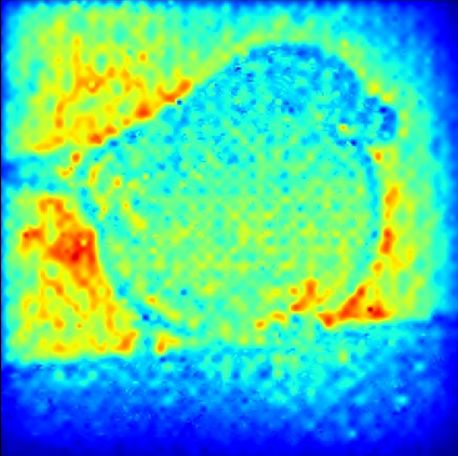
Under review as a conference paper at ICLR 2022

Since predictability is so crucial, why are existing methods not able to achieve it? In fact, saliency
has a degree of predictability since it represents the local behaviors of models, and if we slightly per-
turb the input, the output will perform as shown in saliency. However, such predictability disappears
when many strategies are used to improve its lucidity, like modifying the backpropagation rules,
aggregating the results of different inputs, combining middle activations and backpropagations, and
etc. These methods increase lucidity while changing the functionality in an ambiguous way, so we
cannot predict the attribution behaviors as before.
Is there a method enjoying lucidity and predictability? Guided BackPropagation (GBP) (Springen-
berg et al., 2014) might be a good answer as it visualizes well and has a reconstruction theory (Nie
et al., 2018) justifying its behaviors. However, GBP has two fidelity problems: the class-insensitivity
(Mahendran & Vedaldi, 2016) and the independency of the model parameters (Adebayo et al., 2018).
If we also use heuristic strategies as before, we may run the risk of compromising predictability.
Therefore, we propose a new approach that no longer optimizes attribution performance directly,
but addresses the issues of the reconstruction theory, so-called TR-GBP(Theoretical Refinements of
Guided BackPropagation). As a consequence, TR-GBP can solve fidelity problems without losing
lucidity or predictability. Our main contributions can be summarized three-fold:

       • In addition to lucidity and fidelity, we introduce a novel and critical property predictability
         for BP-based feature attributions.
       • We propose a new predictable feature attribution method TR-GBP, by addressing two fun-
         damental issues in the reconstruction theory of GBP.
       • Qualitative and quantitative experiments are performed and show that TR-GBP can obtain
         sharper visualizations, get rid of the fidelity problems of GBP, and enables us to discrimi-
         nate some prediction errors from interpretation errors.

2     P REDICTABILITY OF F EATURE ATTRIBUTION

To get a predictable interpretation, the definition and requirements of predictability should be clari-
fied. In this section, we specify the scope of predictability and provide some specific predictability
tasks. Then, we show why heuristic strategies fail to predict behaviors and obtain some tips for
keeping predictability when improving the attribution methods.

2.1   D EFINITION OF P REDICTABILITY

Scopes As a reference, in another area, predictability refers to the degree that correct forecasting
can be made (Xu et al., 2019). But for BP-based attributions, the forecasting tasks are not naturally
determined, so we need to specify the scope of the tasks. Considering that the ultimate goal of model
explanations is helping people understand and trust the target models, we focus on the attribution
results that can be clearly perceived by humans and the status of the components which decide
the decision processes. Specifically, the interpretation results that humans can perceive need to
be easily described like intensity changes, shapes, noise, edges, completeness of regions, and etc,
while the components that associate with decision processes of a model normally involve model
inputs, weights, activations, connections of neurons, and etc. Therefore, predictability can be defined
intuitively as the capabilities to predict the human-understandable interpretation behaviors of a given
decision-making process.
Measurements After clarifying the definition, how to measure the predictability of an attribution
method? Due to the difficulties of constructing a general evaluation framework, we only choose
a class of queries which satisfy the human-understandable and are related to the target decision-
making process, like how much noise may appear in the interpretation results? What might happen
when we let some of the model weights be randomly initialized? If there is an unrelated dependency
in the explanation results, does it originate from the model prediction errors or from the explanation
itself? How are attribution results actually connected to decision-making? These questions are not
trivial for BP-based methods, so predictability can be shown as the capabilities of answering these
questions with theoretical analysis.

                                                   2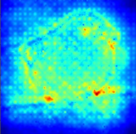
Under review as a conference paper at ICLR 2022

2.2   R EQUIREMENTS OF P REDICTABILITY

As the scopes and tasks of predictability have been clarified, we will next look at what kind of at-
tributions can keep predictability. Recently, there are roughly three kinds of improvement strategies
of BP-based attributions: modifying the backpropagation rules, aggregating the results of different
inputs, and combining middle activations with backpropagations.
Modifying BP-rules These methods modify the backpropagation rules to obtain noise-less attri-
bution results, like Deconv(Zeiler & Fergus, 2014), Guided Back Propagation(GBP) (Springenberg
et al., 2014), Layer-wise relevance propagatoin(LRP) (Bach et al., 2015), ExcitationBP (Zhang et al.,
2018), DeepLIFT (Shrikumar et al., 2017), DeepTaylor(Montavon et al., 2017), PatternAttribution
(Kindermans et al., 2017), Bias Backpropagation(BBp) (Wang et al., 2019), FullGrad (Srinivas &
Fleuret, 2019). However, these changes of backpropagation rules will certainly alter the attribution
behaviors, so these methods no longer represent the local behaviors in a small neighbor of a given
input, and we cannot specify the functionalities of them until another theory is proposed to justify
the behaviors, just like GBP.
Aggregating Gradients Some methods attempt to alleviate gradient issues with the help of the
other input gradients, like SmoothGrad (Smilkov et al., 2017) VarGrad(Adebayo et al., 2018) Inte-
gratedGradients (IG) (Sundararajan et al., 2017) BlurIG(Xu et al., 2020) Guided IntegratedGradients
(GIG) (Kapishnikov et al., 2021). Note that these methods are all unstable as the choices of other
inputs are not determined and different choices might result in different attributions. Therefore,
predictability is ruined by uncertainty.
Activation-based Attributions Activation-based explanations provide attributions for a single in-
put with a linear weighted combination of activation maps from convolutional layers, like Class
Activation Mapping(CAM) (Zhou et al., 2016), GradCAM (Selvaraju et al., 2017), GradCAM++
(Chattopadhay et al., 2018), NormGrad (Rebuffi et al., 2020), CAMERAS (Jalwana et al., 2021).
Remindering that the target convolutional networks are highly non-linear and usually seen as black-
boxes, the middle-layer activation maps of CNNs are also blackboxes. Then, the use of activation
maps will make these methods have unpredictable components.
In all, these improvement strategies can enhance lucidity, but all fail at predictability. So if we want
to optimize an attribution approach, we should find a new way that can insure rigorous functionality,
attribution stability, and without unpredictable components.

3     BACKGROUND
As our proposed method is based on the reconstruction theory (Nie et al., 2018), we introduce its
main conclusions and the core steps of proofs before further discussions.

3.1   P RELIMINARY

Let us start by defining some notations. Consider a multi-category classification with K-class,
suppose there is a d-dimensional image x = {x1 , ..., xd } ∈ Rd , its label is y ∈ {1, ..., K}, for
convenience, we study nomalized input ||x|| = 1. We put x into a deep neural network function
f : Rd 7→ RK , then the attribution map for k th class is Rk : Rd 7→ Rd . Specifically, W l is the
weight of lth layer of f , Al is a vector of the activations of lth layer, and DNN f has L layer. We
have the forward propagation:
                                          Al = σ(W l T Al−1 )                                     (1)
        0
where A = x. The ReLU function is a widely used activation function σ(x) = (x, 0)+ :
                                                       L−1
                                                       Y
                        f = W L T AL−1 = W L T (              M (L−l) W (L−l) T )x                  (2)
                                                        l=1

where M l = diag(I(W l T Al−1 )) denotes the gradient mask of the ReLU operation, I(·) output 1 if
input greater than 0, else output 0. Then the original gradient attribution is:
                                                    L−1
                                           ∂fk    Y
                                    Rk =       =(   W l M l )vk                                     (3)
                                           ∂x
                                                       l=1

                                                   3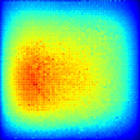
Under review as a conference paper at ICLR 2022

where vk is k th row of W L T which can produce the k th output. For GBP, the negative gradi-
ents passing through the activation functions will be zero-out with the help of ReLU operation, see
Figs.1(b):
                                                L−1
                                       ∂ g fk    Y
                                Rk = g = (           (W l )M l σ◦)vk                            (4)
                                       ∂ x
                                                      l=1

3.2   R ECONSTRUCTION T HEORY OF GBP

There are two main results of reconstruction theory (Nie et al., 2018): one is a theorem for three-layer
CNNs and the other is a proposition for expanding to deeper networks. Now we consider a three-
layer CNN, consisting of an input layer, a convolutional hidden layer and a fully connected layer.
Let W ∈ Rp×N be N convolutional filters and we denote each column w(i) as the i-th filter with
size p. Then, we let C ∈ Rp×J be J image patches extracted from x, and each column c(j) with size
p is generated by a linear function c(j) = Dj x where Dj , [0p×(j−1)s Ip×p 0p×(d−(j−1)s−p) ] with
s being the stride size. The weights in the fully connected layer can be represented by V ∈ RN J×K .
Therefore, the k-th logit is represented by
                                            N X
                                            X J
                                 fk (x) =             Vqij ,k σ(w(i)T c(j) )                              (5)
                                            i=1 j=1

where the index qij denotes the ((i − 1)J + j)-th entry in every column vector of weight matrix V .
Theorem 1. Considering a three layer ReLU convolutional network with sufficient large like
Eqn.(5), and the elements of V and W are all assumed to be independently Gaussian distributed
with zero mean and variance c2 , Z is the normalized term, and GBP at the k-th logit is:
                                             J      N
                                 ∂ g fk   1 X T X (i)
                    sGBP
                     k   (x) =          =       Dj     w I(w(i) c(j) )σ(Vqij ,k )                         (6)
                                 ∂g x     Z j=1    i=1

Then, the GBP at the k-th logit can be approximated as:
                                                            2c2 pN
                                         sGBP
                                          k   (x) ≈                x                                      (7)
                                                            πC0 Z
where C0 = ||c(j) ||2 and if we assume they are the same for all j, then use the normalization term
Z = 2cπC               GBP
       2 pN , we have sk
          0
                            (x) ≈ x.

Nie et al. (2018) provide a proof of Theorem 1, and now we briefly demonstrate the
key proof steps: (1) They transform the summations into the mean of filter weights:
PN       (i)    (i) (j)                 1
                                          PN        (i)  (i) (j)
   i=1 w I(w c )σ(Vqij ,k ) = N N            i=1 w I(w c )σ(Vqij ,k ). (2) They estimate this mean
                                                                   PN
with the help of the expectation of weight distributions: N1 i=1 w(i) I(w(i) c(j) )σ(Vqij ,k ) ≈
E(w(i) I(w(i) c(j) )σ(Vqij ,k )). (3) Note that all the weights sampled i.i.d, the expectations can be
split into a product of two items: E(w(i) I(w(i) c(j) )) and E(σ(Vqij ,k )). (4) E(σ(Vqij ,k )) are con-
                                                       2c2 p
stant positive values and E(w(i) I(w(i) c(j) )) =   π||c(j) ||2 Z
                                                                  c(j)   due to the ReLU operations block the
                                                                         (j)
convolutional kernels in the opposite directions to the input c , as illustrated in Figs.2(a), the blue
arrow represents the input vector where the red arrows mean the weights of convolutional kernels,
and a plane perpendicular to input vector blocks out the red arrows which have a large angle with
the input. Note that the weights are i.i.d. drawn from Gaussian distributions, the expectations of the
rest weights will converge in the same direction as input. (5) If we assume C0 = ||c(j) ||2 , each piece
c(j) are then arranged according to conventional operations (see Figs.2(b)) and finally normalized to
the input x. This result can also be expanded to more than three layers:
Proposition 1. For a random deep CNN where weights are i.i.d. Gaussians with zero mean, we can
                                                                                       g
also approximate every entry of Ṽ as i.i.d. Gaussian with zero mean, where Ṽ = ∂∂g Afk1 denotes the
backpropation results to the first activation maps.

The core of this proof is the Gaussian distribution with zero mean, which can use the Central Limit
Theorem to obtain. It can be seen that under this theory the functionalities and behaviors of GBP

                                                      4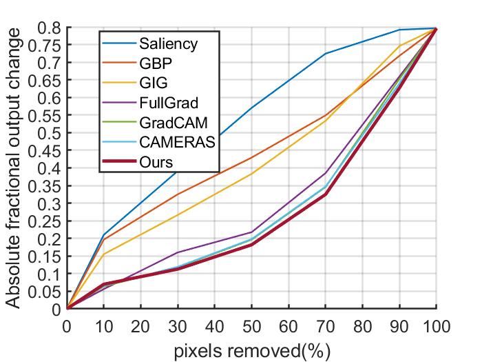
Under review as a conference paper at ICLR 2022

have a theoretical justification for predictions, but a reconstruction might not be a good attribution:
the reconstruction represents the use of input information. Note that the predictions of different
classes might share similar information, such reconstructions fail to highlight the differences which
determine the decision making. In addition, previous work finds that GBP stays identical even if
the top layers are randomized (Adebayo et al., 2018). These fidelity issues illustrate the functional
deficiencies of the GBP.

4     T HEORETICAL R EFINEMENT OF GBP
4.1   A DDRESSING THE L IMITATIONS OF R ECONSTRUCTION T HEORY

Next, we are going to complement some improvements of GBP to obtain fidelity without losing pre-
dictability. According to the requirements listed in Section 2.2, keeping predictability needs a theory
justifying the behaviors, and the improvements should not apply instable or unpredictable compo-
nents. Therefore, we decide to obtain ideas for improvements by addressing theoretical shortcom-
ings, so that our changes can also be estimated with this theory. Specifically, we find two limitations:

       • The missing of bias terms: As reconstruction theory does not take the widely adopted
         bias terms into consideration, its conclusions cannot be directly applied to traditional net-
         works. As bias terms also contribute to decision-making processes (Srinivas & Fleuret,
         2019; Wang et al., 2019), the missing of bias terms will make attribution results incomplete
         and ignore the high-layer changes. That is why GBP failed the sanity checks (Adebayo
         et al., 2018).
       • The similarity of Ṽ : according to the central limited theorem and the Proposition 1, the
         backpropagation results might have similar distributions for different vk , and so that GBP
         is class-insensitive (Sixt et al., 2020).

These limitations are obvious and gravely affect the fidelity of GBP. Now, we will provide two
straight forward strategies without any instable or unpredictable component like other inputs or
middle-layer activations. Our improvements are as follows:
(a) Treatment of bias terms: We apply an operation commonly used in machine learning to transform
the bias term into additional input 1: f (x) = V σ(W x + b) = V σ(Ŵ x̂), where Ŵ = [W, b],
x̂ = [x, 1]T . As for convolutional networks, the additional input 1 will also transform to patches, as
illustrated in Figs.1(b):
                  N X
                    J                                     N X
                                                            J
                  X                                       X                                    bT
       fk (x) =             Vqij ,k σ(w(i)T Dj x + b) =             Vqij ,k σ(w(i)T Dj x +           Dj 1)   (8)
                  i=1 j=1                                 i=1 j=1
                                                                                             ||Dj ||

where b is a p-dimensional vector filled with b. Therefore, the reconstruction of input x in Theorem 1
                                                                                    g k
can be divided into two parts: the recovery of input image x, denoted as R̃k0 = ∂∂ gfx , and the recovery
                                            g
of lth layer input 1l , denoted as R̃kl = ∂∂ gf1kl . Then, if we apply the GBP to a model, we need not
only obtain the GBP for input image x, but also the middle layer input 1, as shown in Figs.1(a).
Considering that the model captures different levels of input features, the reconstruction of middle
layer 1 can reflect the reconstruction abilities at different levels. Note that the final attribution maps
must keep the same size of the input x, we aggregate these results with the spatial pior introduced
by GradCAM (Selvaraju et al., 2017):
                                        X                 ∂ g fk X ∂ g fk
                           R̃k = R̃k0 +      ψ(R̃kl ) = g +           ψ(         )                     (9)
                                         l
                                                           ∂ x
                                                                    l
                                                                          ∂ g 1l
where ψ(·) = BilinearU psample(·).
(b) Removing similarities shared by different classes: The goal of attribution is to explain why the
model makes a certain decision, so we should focus on what is different across classes, rather than
the similar information:
                                                         K
                                                      1 X
                                    Rk (x) = R̃k −          R̃i                                 (10)
                                                     K i=1

                                                     5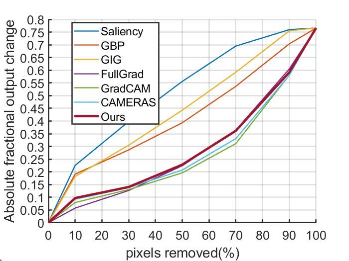
Under review as a conference paper at ICLR 2022

                (a) Forward propagation                           (b) Backward propagation

Figure 1: Pipeline of TR-GBP. The forward propagation treats the bias as input maps fullfilled with
1, and the back propagation procedure also attribute to the middle inputs. Then we aggregate these
middle input with upsampling, and minus the mean values of top5 results.

                                                           (a) input    (b) bull mastiff     (c) tiger cat

 (a) Input alignment      (b) Convolution              Figure 3: Class discriminative results for TR-
                                                       GBP. The middle heatmap is obtained from the
Figure 2: The illustration of important opera-         class ‘bull mastiff’, and the right heatmap is ob-
tions.                                                 tained from the class ‘tiger cat’.

In practice, categories with low prediction probabilities might not have any activated M L in Eqn.(2),
so their backpropagations might be set to zero after the fc-layer, and fail to reflect the shared infor-
mation. In this work, we therefore remove the mean value of the top5 classes for avoid such absences
and achieve computational efficiency. Now, we finally obtain an attribution method Rk , and call it
TR-GBP (Theoretical Refinements of Guided BackPropagation). If we want to get different levels of
                                                                                            1
                                                                                              PK
attribution, we can also apply such operation to the middle-layer results: Rkl (x) = R̃kl − K         l
                                                                                                i=1 R̃i .
                                                                         0              l
                                                                               P
According to the exchangeability of linear operators, we have Rk = Rk + l ψ(Rk ). The pipeline
of TR-GBP is illustrated in Figs.1(b), it can be seen that the puck class uses the information of head
and sticks, but if we remove the means of top5 classes: puck, ski, ballplayer, knee pad, helmet, the
attribution results become jersey and sticks, as head information is shared with ballplayer or helmet.

4.2   T HE P REDICTABILITY OF TR-GBP

As predictability has been concretized to some questions in Section 2, we now show how much
predictability TR-GBP achieves by answering these questions:
(1) How much noise may appear in the interpretation results?
The noise is from the step (2) in Section 3.2, since the estimate of the expectations may introduce
differences in randomness.PFrom (Lugosi & Mendelson, 2019), We can set N = Õ(p/2 ) such that
with high probability || N1 i=1 N I(w(i) c(j) ) − E(I(w(i) c(j) )|| < , where p denotes the filter size
and Õ(·) hides some other factors. So filter size p and filter num N are the dominant factors for
noise. As the top layer normally has larger N , there must be less noise on the top-layer attributions
than the bottom-layer results. This phenomenon can be found in Appendix B.
(2) What might happen to the interpretation results when we let some of the model parameters be
randomly initialized?
According to Theorem 1, if all the weights are randomly initialized, the result will be a recovery
of input. As the middle-layer inputs are feature maps fullfilled with 1, the reconstruction will also

                                                   6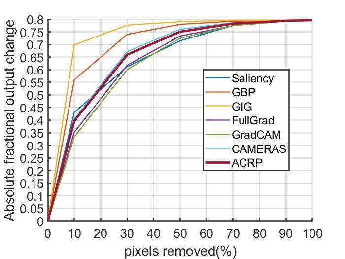
Under review as a conference paper at ICLR 2022

            Input   Saliency     GBP        GIG       FullGrad    GradCAM CAMERAS             Ours

VGG16
ResNet50

Figure 4: Visualization results on VGG16 and ResNet50 of saliency, GBP, GIG, FullGrad, Grad-
CAM, CAMERAS and our method TR-GBP.

be nearly uniform. Note that boundary inputs usually have less convolutional operators, as shown
in Figs.2(b), the center inputs participate 9 convolutions while the corner inputs only have 4 con-
volutions. So the reconstruction will produce weaker attributions at the boundaries. Therefore, if
we cascadely randomize the weights from top layer to the bottom layer, the middle attributions will
gradually become uniform. Such phenomenon is shown in Section 5.2.2 and Appendix B.
(3) When there is an unrelated dependency in the explanation results, does this dependency originate
from the prediction errors of the model or from the explanation itself?
Note that we have predicted that the boundaries of attribution must be weaker, so if there are high
scores in boundaries, it must originate from prediction errors. This claim is supported by the results
of Section 5.4.

5          E XPERIMENTS

In this section, we conduct experiments to show that our method can keep lucidity, fidelity, and
predictability simultaneously.

5.1        V ISUAL I NSPECTION

We perform qualitative visual evaluation for TR-GBP along with baselines on validation set of Ima-
geNet: saliency, GBP, GIG, GradCAM, FullGrad, CAMERAS. These methods are the newest or the
most classical attribution methods of three kinds of attributions listed in Section 2.2. Furthermore,
we use the commonly used pretrained models: VGG16 and ResNet50 from torchvision model zoo.
The results are shown in Figure 4, it can be seen that saliency is full of noise, GBP and GIG highlight
the edges and FullGrad, GradCAM, TR-GBP shed light on a complete region. This is not surprising
that TR-GBP is more complete than GBP and more tightly confined to object regions than Grad-
CAM, FullGrad, CAMERAS, because we supplement the bias attributions for GBP and theoretical
guarantee low noise level in Section 4.2.

5.2        F IDELITY P ROBLEMS

Note that GBP has found two fidelity problems in previous studies, we need to show that TR-GBP
can solve them effectively with our theoretical refinements.

                                                  7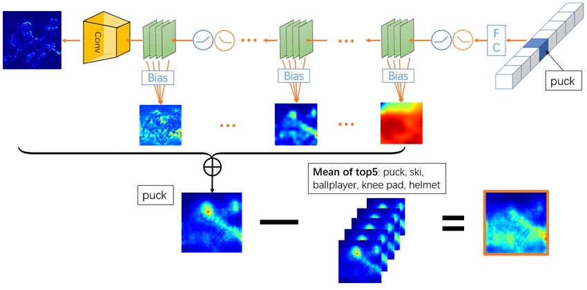
Under review as a conference paper at ICLR 2022

  (a) input     (b) raw      (c) fc    (d) layer4       (e) layer3     (f) layer2    (g) layer1   (h) conv1

Figure 5: Sanity check results by cascade randomizing resnet50 from fc layer to the conv1 layer for
TR-GBP.

         Table 1: Comparative evaluation on Energy-Based Pointing Game (higher is better).
  Model(%)      Saliency   GBP        GIG           FullGrad         GradCAM        CAMERAS        Ours
  VGG           40.2±0.3   56.1±0.4   41.2±0.6      41.3±0.4         45.7±1.1       45.9±1.0      52.2±1.4
  ResNet        36.9±0.5   55.4±0.5   40.6±0.7      35.0±0.6         40.8±1.0       50.1±1.2      53.4±1.1

5.2.1    C LASS D ISCRIMINATIVE V ISUALIZATION
Figure 3 shows our results on cat and dog image for ResNet50. The top1 class of output is ’bull
mastiff’ and the top2 class is ’tiger cat’. It is evident that our method can distinguish different
classes, and provide entire objects except for the tail of the cat. Such results are reasonable as we
remove the reconstruction shared by different categories. More comprehensive results about class
discriminative visualizations can be seen in Appendix A.

5.2.2    S ANITY C HECKS
Adebayo et al. (2018) point out that some attribution methods are not able to show the differences
between different models, just like special edge detectors. Specifically, they randomize some layers
of model, and find that some attribution results, especially GBP, almost remain unchanged. We also
perform a sanity check of TR-GBP and present the results in Figure 5. As can be seen, our method
is sensitive to model parameters and can efficiently reflect the differences between models before
and after randomization. Moreover, the attribution results of TR-GPB converge to uniform with
weak boundaries and random noises. This phenomenon just supports the analysis of predictability
question (2) in Section 4.2. Other results can be seen in Appendix B.

5.3     Q UANTITATIVE E VALUATIONS

5.3.1    L OCALIZATION A BILITIES
Wang et al. (2020) provide an Energy-Based Pointing Game (EBPG) to evaluate the localization
ability of attribution methods. Such evaluation reflects whether the highlighting regions of method
are consistent with humans. Specifically, the evaluation is attributed inside the bounding boxes as a
proportion of all attributions:
                                                  P
                                                     Rx∈bbox
                                EBP G = P                 P                                     (11)
                                              Rx∈bbox + Rx∈bbox   /

The experiment settings are shown in Appendix C, and the evaluation results of VGG16 and
ResNet50 are reported in Table 1. TR-GBP outperforms all other baseline attribution methods sig-
nificantly, except GBP. That is because GBP is only part of our attribution and loses a lot of useful
information: for example, our method finds many boundary dependencies which associate with pre-
diction errors in Section 5.4, but GBP discards middle-layer information and lacks this capability.

5.3.2    P IXEL P ERTURBATIONS
Pixel perturbations (Samek et al., 2016) are evaluations which remove the most or least impor-
tant pixels and compare the magnitude of the changes to judge whether the interpretation results
effectively describe the models. We perform two kinds of pixel perturbations on Imagenet 2012

                                                    8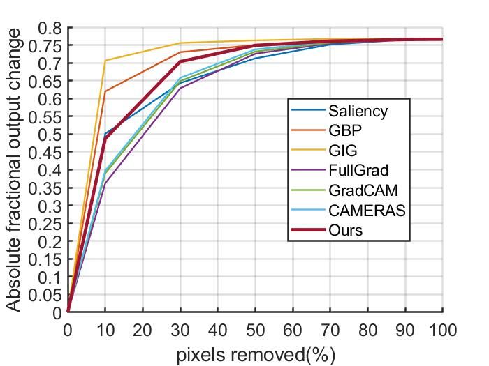
Under review as a conference paper at ICLR 2022

      (a) VGG+MoRF             (b) VGG+LeRF            (c) ResNet+MoRF          (d) ResNet+LeRF

Figure 6: Pixel perturbation results on Imagenet 2012 validation set with VGG16 and ResNet50,
both removing most relevant features(MoRF,higher is better) and removing least relevant fea-
tures(LeRF, lower is better).

                Table 2: Comparative evaluation on AUC of IBD (higher is better).
       Model(%)     Saliency    GBP     GIG      FullGrad    GradCAM       CAMERAS        Ours
       VGG          52.84       53.03   53.85    53.72       56.86         57.00          60.95
       ResNet       51.44       51.96   53.79    54.04       53.06         54.99          62.16

validation dataset: removing most relevant input features (MoRF) and removing least relevant input
features (LeRF) Samek et al. (2016). More details of experiments can be found in Appendix D. The
results are shown in Figure 6, as can be seen, our method shows the best result for ResNet+LeRF,
outperform CAMERAS, GradCAM, Fullgrad for all MoRF, and obtains comparable performance in
VGG+LeRF.

5.4   VALIDATE P REDICTABILITY

Let us look closely at the results of Figs.5(b) and (c), the changes of fc layer lead to high scores in
boundaries. According to the answers to predictability question (3) in Section 4.2, as we have pre-
dicted that the boundaries of attribution must be weaker, if there are high scores in boundary pixels
of TR-GBP, it must originate from model prediction errors. Note that such boundary dependencies
are also shown by previous methods, like CAMERAS in Figs.4. Therefore, we attempt to conduct
validation experiments to make sure such boundary dependencies in our method are actually a pre-
diction errors but others not. Specifically, we use a metric which is similar to EBPG to represent the
intensities of boundary dependencies (IBD):
                                                 P
                                                    Rx∈boundary
                             IBD = P                       P                                      (12)
                                          Rx∈boundary + Rx∈boundary
                                                                /

where boundary is the 16-pixel boundary regions: height, width < 16 or height, width > 224 −
16. We dicard half data in ImageNet validation set with the minimal IBD to obtain attribution
results with salient boundary dependencies. Note that the dependency originates from prediction
errors must have capacities to show the correctness of predictions, so we use traditional AUC (Area
Under Curve) values of ROC curve to measure whether IBD can be used as a valid indicator to judge
the correctness of model predictions. The results are shown in Table 2. TR-GBP has remarkable
advance performance, which means that the boundary dependencies in TR-GBP are actually derived
from prediction errors while other methods not, so TR-GBP succeeds in disentangling prediction
errors from interpretation errors with the help of predictability.

6     C ONCLUSION
In this work, we propose a novel and important concept Predictability for BP-based attributions,
and a new attribution method, named TR-GBP, which addresses the issues of reconstruction theory
rather than intuitive improvements of performance to improve lucidity and fidelity while ensuring
predictability. The experiments on ImageNet show that TR-GBP achieves lucid visualization and
solves two fidelity problems. In addition, the answers to predictability questions are all supported
by experimental phenomena, so TR-GBP is a predictable attribution method to a certain extent. In
the feature, we plan to obtain quantitative evaluations for predictability.

                                                  9
Under review as a conference paper at ICLR 2022

R EFERENCES
Julius Adebayo, Justin Gilmer, Michael Muelly, Ian Goodfellow, Moritz Hardt, and Been Kim.
  Sanity checks for saliency maps. arXiv preprint arXiv:1810.03292, 2018.
Sebastian Bach, Alexander Binder, Grégoire Montavon, Frederick Klauschen, Klaus-Robert Müller,
  and Wojciech Samek. On pixel-wise explanations for non-linear classifier decisions by layer-wise
  relevance propagation. PloS one, 10(7):e0130140, 2015.
Tathagata Chakraborti, Anagha Kulkarni, Sarath Sreedharan, David E Smith, and Subbarao Kamb-
  hampati. Explicability? legibility? predictability? transparency? privacy? security? the emerging
  landscape of interpretable agent behavior. In Proceedings of the international conference on au-
  tomated planning and scheduling, volume 29, pp. 86–96, 2019.
Aditya Chattopadhay, Anirban Sarkar, Prantik Howlader, and Vineeth N Balasubramanian. Grad-
  cam++: Generalized gradient-based visual explanations for deep convolutional networks. In 2018
  IEEE winter conference on applications of computer vision (WACV), pp. 839–847. IEEE, 2018.
Mohammad AAK Jalwana, Naveed Akhtar, Mohammed Bennamoun, and Ajmal Mian. Cameras:
 Enhanced resolution and sanity preserving class activation mapping for image saliency. In Pro-
 ceedings of the IEEE/CVF Conference on Computer Vision and Pattern Recognition, pp. 16327–
 16336, 2021.
Andrei Kapishnikov, Subhashini Venugopalan, Besim Avci, Ben Wedin, Michael Terry, and Tolga
  Bolukbasi. Guided integrated gradients: An adaptive path method for removing noise. In Proceed-
  ings of the IEEE/CVF Conference on Computer Vision and Pattern Recognition, pp. 5050–5058,
  2021.
Harmanpreet Kaur, Harsha Nori, Samuel Jenkins, Rich Caruana, Hanna Wallach, and Jennifer Wort-
  man Vaughan. Interpreting interpretability: Understanding data scientists’ use of interpretability
  tools for machine learning. In Proceedings of the 2020 CHI Conference on Human Factors in
  Computing Systems, pp. 1–14, 2020.
Pieter-Jan Kindermans, Kristof T Schütt, Maximilian Alber, Klaus-Robert Müller, Dumitru Erhan,
  Been Kim, and Sven Dähne. Learning how to explain neural networks: Patternnet and patternat-
  tribution. arXiv preprint arXiv:1705.05598, 2017.
Gábor Lugosi and Shahar Mendelson. Sub-gaussian estimators of the mean of a random vector. The
  annals of statistics, 47(2):783–794, 2019.
Aravindh Mahendran and Andrea Vedaldi. Salient deconvolutional networks. In European Confer-
  ence on Computer Vision, pp. 120–135. Springer, 2016.
Grégoire Montavon, Sebastian Lapuschkin, Alexander Binder, Wojciech Samek, and Klaus-Robert
  Müller. Explaining nonlinear classification decisions with deep taylor decomposition. Pattern
  Recognition, 65:211–222, 2017.
Weili Nie, Yang Zhang, and Ankit Patel. A theoretical explanation for perplexing behaviors of
 backpropagation-based visualizations. In International Conference on Machine Learning, pp.
 3809–3818. PMLR, 2018.
Sylvestre-Alvise Rebuffi, Ruth Fong, Xu Ji, and Andrea Vedaldi. There and back again: Revisiting
  backpropagation saliency methods. In Proceedings of the IEEE/CVF Conference on Computer
  Vision and Pattern Recognition, pp. 8839–8848, 2020.
Wojciech Samek, Alexander Binder, Grégoire Montavon, Sebastian Lapuschkin, and Klaus-Robert
 Müller. Evaluating the visualization of what a deep neural network has learned. IEEE transactions
 on neural networks and learning systems, 28(11):2660–2673, 2016.
Ramprasaath R Selvaraju, Michael Cogswell, Abhishek Das, Ramakrishna Vedantam, Devi Parikh,
  and Dhruv Batra. Grad-cam: Visual explanations from deep networks via gradient-based local-
  ization. In Proceedings of the IEEE international conference on computer vision, pp. 618–626,
  2017.

                                                10
Under review as a conference paper at ICLR 2022
Avanti Shrikumar, Peyton Greenside, and Anshul Kundaje. Learning important features through
propagating activation differences. In International Conference on Machine Learning, pp. 3145–
3153. PMLR, 2017.
Karen Simonyan, Andrea Vedaldi, and Andrew Zisserman. Deep inside convolutional networks: Vi-
sualising image classification models and saliency maps. arXiv preprint arXiv:1312.6034, 2013.
Leon Sixt, Maximilian Granz, and Tim Landgraf. When explanations lie: Why many modified bp
attributions fail. In International Conference on Machine Learning, pp. 9046–9057. PMLR, 2020.
Daniel Smilkov, Nikhil Thorat, Been Kim, Fernanda Viégas, and Martin Wattenberg. Smoothgrad:
removing noise by adding noise. arXiv preprint arXiv:1706.03825, 2017.
Jost Tobias Springenberg, Alexey Dosovitskiy, Thomas Brox, and Martin Riedmiller. Striving for
simplicity: The all convolutional net. arXiv preprint arXiv:1412.6806, 2014.
Suraj Srinivas and François Fleuret. Full-gradient representation for neural network visualization.
arXiv preprint arXiv:1905.00780, 2019.
Akshayvarun Subramanya, Vipin Pillai, and Hamed Pirsiavash. Fooling network interpretation in
image classification. In Proceedings of the IEEE/CVF International Conference on Computer
Vision, pp. 2020–2029, 2019.
Mukund Sundararajan, Ankur Taly, and Qiqi Yan. Axiomatic attribution for deep networks. In
International Conference on Machine Learning, pp. 3319–3328. PMLR, 2017.
Hideomi Tsunakawa, Yoshitaka Kameya, Hanju Lee, Yosuke Shinya, and Naoki Mitsumoto. Con-
trastive relevance propagation for interpreting predictions by a single-shot object detector. In 2019
International Joint Conference on Neural Networks (IJCNN), pp. 1–9. IEEE, 2019.
Haofan Wang, Zifan Wang, Mengnan Du, Fan Yang, Zijian Zhang, Sirui Ding, Piotr Mardziel, and
Xia Hu. Score-cam: Score-weighted visual explanations for convolutional neural networks. In
Proceedings of the IEEE/CVF Conference on Computer Vision and Pattern Recognition Work-
shops, pp. 24–25, 2020.
Shengjie Wang, Tianyi Zhou, and Jeff Bilmes. Bias also matters: Bias attribution for deep neural
network explanation. In International Conference on Machine Learning, pp. 6659–6667. PMLR,
2019.
Paiheng Xu, Likang Yin, Zhongtao Yue, and Tao Zhou. On predictability of time series. Physica A:
Statistical Mechanics and its Applications, 523:345–351, 2019.
Shawn Xu, Subhashini Venugopalan, and Mukund Sundararajan. Attribution in scale and space.
In Proceedings of the IEEE/CVF Conference on Computer Vision and Pattern Recognition, pp.
9680–9689, 2020.
Matthew D Zeiler and Rob Fergus. Visualizing and understanding convolutional networks. In
European conference on computer vision, pp. 818–833. Springer, 2014.
Jianming Zhang, Sarah Adel Bargal, Zhe Lin, Jonathan Brandt, Xiaohui Shen, and Stan Sclaroff.
Top-down neural attention by excitation backprop. International Journal of Computer Vision, 126
(10):1084–1102, 2018.
Bolei Zhou, Aditya Khosla, Agata Lapedriza, Aude Oliva, and Antonio Torralba. Learning deep
features for discriminative localization. In Proceedings of the IEEE conference on computer
vision and pattern recognition, pp. 2921–2929, 2016.
11Under review as a conference paper at ICLR 2022
Raw Irish terrier Norwich terrier Australian terrier Airedale terrier Lakeland terrier
(a)
Raw bull mastiff boxer tiger affenpinscher tiger cat
(b)
Raw soccer ball tennis ball Lhasa Shih-Tzu toy poodle
(c)
Raw junco brambling house finch water ouzel indigo bunting
(d)
Figure 7: Class Discriminative Visualization for VGG16. From left to right, they represent top1-top5
classes.
A A PPENDIX
A C LASS D ISCRIMINATIVE V ISUALIZATIONS
There are class discriminative visualizations for VGG16 and ResNet50 models. We show the top 5
classes results of TR-GBP in Figure 7 and Figure 8. We use Relu function to highlight the regions
which have superior reconstructive abilities than average for the given class. It is shown that TR-
GBP can highlight the correct regions for target classes according to their meaning, while absence
class would be below the average. For example, in Figure 7(a), the ears of dogs attribute much to
Norwich terrier class. In Figure 1(b), all the dog classes highlight the region of dog, and the class of
tiger or cat highlights the region of cat. In Figure 7(c), soccer ball and tennis ball show the attention
on ball, Lhasa, and etc. show the attention on dog. In Figure 7(d), the junco class is so outstanding
that other classes are all below the average. We can also find similar results in Figure 8. These results
show that our method can effectively capture the model preferences of input features for different
classes.
12Under review as a conference paper at ICLR 2022
Raw Irish terrier Airedale Lakeland terrier Australian terrier fox terrier
(a)
Raw bull mastiff tiger cat boxer tabby cat doormat
(b)
Raw bobtail soccer ball Maltese dog komondor Sealyham
(c)
Raw junco brambling house finch indigo bunting jay
(d)
Figure 8: Class Discriminative Visualization for ResNet50. From left to right, they represent top1-
top5 classes.
B S ANITY C HECKS
In this section, we present more detailed results for sanity check. We show the reconstruction ability
of different layers, and demonstrate the influence of cascade randomization of models on different
layers. The results can be seen in Figure 9 for VGG16, and Figure 10 for ResNet50. It can be seen
that the low layers of model can emerge corresponding features, and then highlight some of them
according to the high-layer attention. In this way, if high layers of a model have been randomized,
the reconstruction of low layer can still recognize and discard some irrelevant input features, until
they have been randomized too, and then become meaningless. It is noticed that VGG has three FC
layers with ReLU activations at the top, according to the answer to predictability questions (1), the
noise level depends on the kernel size p, as the FC-layer can be seen as large kernel convolution,
such p is too large, so the results in 9 also composite with noise at the top attribution results. These
results show that our method can effectively reflect the changes of model parameters.
Additionally, let us concentrate on the columns of ’raw’ in Figure 9 and 10, it is clear that the results
of bottom layers have more noise than top layers, which have been forecasted in Section4.2.
13Under review as a conference paper at ICLR 2022
image raw classifier layer 11 layer 7 layer 4 layer1
(a) Aggregation of all layers
(b) Layer11
(c) Layer7
(d) Layer4
(e) Layer1
Figure 9: Sanity checks for different layers on VGG16. From left to right, it reflects the cascade
randomization of model.
C E XPERIMNENTAL D ETAILS OF E NERGY- BASED P OINTING G AMES
In detail, we use the same setting as Wang et al. (2020): (1) Removing images where an object
occupies more than 50% of the whole image to guarantee the bounding box makes sense; (2) Only
considered the images with one bounding box which represents the target. We experiment on 500
random selected images from the ILSVRC2012 validation set, each term repeats 5 times and obtains
the mean and standard deviation.
D E XPERIMNENTAL D ETAILS OF P IXEL P ERTURBATIONS
Specifically, our procedure is as follows: for a given value of k, we replace the k pixels corresponding
to k most/least salient values with zero pixels. Especially, for GBP and GIG, we add an absolute
function to obtain the least differences for LeRF as the least score is not zero but negative values,
which means it can also influence the output.
14Under review as a conference paper at ICLR 2022
image raw fc layer4 layer3 layer2 layer1
(a) Aggregation of all layers
(b) A layer in Layer4
(c) A layer in Layer3
(d) A layer in Layer2
(e) A layer in Layer1
Figure 10: Sanity checks for different layers on ResNet50. From left to right, it reflect the cascade
randomization of model.
15You can also read