The rise of grasslands is linked to atmospheric CO2 decline in the late Palaeogene - Nature
←
→
Page content transcription
If your browser does not render page correctly, please read the page content below
ARTICLE
                   https://doi.org/10.1038/s41467-021-27897-y                OPEN

                  The rise of grasslands is linked to atmospheric CO2
                  decline in the late Palaeogene
                  Luis Palazzesi         1,2 ✉,   Oriane Hidalgo2,3, Viviana D. Barreda1, Félix Forest2,6 & Sebastian Höhna4,5,6 ✉

                  Grasslands are predicted to experience a major biodiversity change by the year 2100. A
                  better understanding of how grasslands have responded to past environmental changes will
1234567890():,;

                  help predict the outcome of current and future environmental changes. Here, we explore the
                  relationship between past atmospheric CO2 and temperature fluctuations and the shifts in
                  diversification rate of Poaceae (grasses) and Asteraceae (daisies), two exceptionally species-
                  rich grassland families (~11,000 and ~23,000 species, respectively). To this end, we develop a
                  Bayesian approach that simultaneously estimates diversification rates through time from
                  time-calibrated phylogenies and correlations between environmental variables and diversi-
                  fication rates. Additionally, we present a statistical approach that incorporates the informa-
                  tion of the distribution of missing species in the phylogeny. We find strong evidence
                  supporting a simultaneous increase in diversification rates for grasses and daisies after the
                  most significant reduction of atmospheric CO2 in the Cenozoic (~34 Mya). The fluctuations
                  of paleo-temperatures, however, appear not to have had a significant relationship with the
                  diversification of these grassland families. Overall, our results shed new light on our
                  understanding of the origin of grasslands in the context of past environmental changes.

                  1 Museo Argentino de Ciencias Naturales & Consejo Nacional de Investigaciones Científicas y Técnicas (CONICET), Buenos Aires C1405DJR, Argentina.
                  2 Jodrell
                          Laboratory, Royal Botanic Gardens, Kew, Richmond, Surrey TW9 3DS, UK. 3 Institut Botánic de Barcelona (IBB, CSIC-Ajuntament de Barcelona),
                  Catalonia, Spain. 4 GeoBio-Center, Ludwig-Maximilians-Universität München, Richard-Wagner-Str. 10, 80333 Munich, Germany. 5 Department of Earth and
                  Environmental Sciences, Paleontology & Geobiology, Ludwig-Maximilians-Universität München, Richard-Wagner-Str. 10, 80333 Munich, Germany. 6These
                  authors contributed equally: Félix Forest, Sebastian Höhna ✉email: lpalazzesi@macn.gov.ar; hoehna@lmu.de

                  NATURE COMMUNICATIONS | (2022)13:293 | https://doi.org/10.1038/s41467-021-27897-y | www.nature.com/naturecommunications                          1
ARTICLE                                                                 NATURE COMMUNICATIONS | https://doi.org/10.1038/s41467-021-27897-y

T
        he grassland biome (steppes, savannas, and prairies) covers          Supplementary Fig. 6). This diversification rate shift is robust to
        vast areas of the Earth’s surface and today accounts for as          several model assumptions. We recovered the same diversifica-
        much as one-third of the net primary production on                   tion rate shifts regardless of the assumed number of time intervals
land1,2. Although grasses (Poaceae) comprise the bulk of the                 (Supplementary Fig. 7). Both autocorrelated diversification rate
biomass and plant population in grasslands, other plant families—            prior models qualitatively agree on the overall pattern of diver-
in particular the daisies (Asteraceae)—are usually as much as (or            sification rates (Gaussian Markov random field (GMRF) or
even more) diverse than grasses (Supplementary Fig. 1). The                  Horseshoe Markov random field (HSRMF), Supplementary
evolution of grasslands marked the emergence of a new landscape              Figs. 6 and 7). Only the uncorrelated diversification rate prior
and provided the substrate for the adaptive radiation of other life          model differed in the inferred pattern (UCLN, Supplementary
forms that coevolved along with this biome, including grazing                Figs. 6 and 7). However, the autocorrelated diversification rate
mammals3 such as horses, wombats, and capybaras.                             prior models were significantly favored according to our Bayes
   The age of a given biome is often estimated by detecting when             factor analyses (GMRF for the daisy phylogenetic tree and
particular representative taxonomic groups first appear in the                HSMRF for the grass phylogenetic tree, Supplementary Fig. 8).
fossil record. For example, the early evolution of the grassland             Recently, Louca and Pennell28 showed that phylogenies of extant
biome—and open-habitat biomes in general—has been estimated                  taxa are consistent with infinitely many diversification rate
from the fossil record of grass phytoliths (plant silica)4 or from           models and therefore diversification rates are not identifiable if
the record of fossil pollen of daisies, grasses, and amaranths5,6.           arbitrarily complex diversification rate functions are allowed. Our
Phylogenetic trees based on DNA sequence data calibrated with                diversification models, on the other hand, are identifiable because
fossils provide a powerful new perspective on the history of                 of the piecewise-constant (episodic) diversification rates model29.
biomes7. This approach has been used to estimate the timing of               Furthermore, model comparison is robust when well-formulated
tropical-rainforest evolution based on phylogenetic trees of plant           alternative hypotheses are used30, as is the case for the compar-
groups that are characteristic of this biome (e.g., Malpighiales8,           ison between different environmentally dependent diversification
Arecaceae9, and the legume genus Inga10). Nevertheless, phylo-               models31.
genetic approaches have barely been used to study the evolu-                    The diversification rate patterns were strongly influenced by
tionary history of grassy biomes; most previous studies of                   the assumed incomplete taxon sampling (Supplementary Fig. 9).
grassland evolution have focused on the origins of C4                        In our simulation study we show that incorrectly assuming uni-
grasslands11. Here we estimate when grasslands first expanded                 form taxon sampling and thus disregarding taxonomic informa-
using phylogenetic trees of its two primary plant families, Poaceae          tion about the distribution of missing species strongly biases
and Asteraceae. We assembled a large calibrated phylogenetic tree            diversification rates (Supplementary Figs. 22 and 23). Conversely,
for daisies and used the largest tree yet inferred for grasses11 to          our empirical taxon sampling informed by a more accurate dis-
explore temporal shifts in rates of lineage diversification, and to           tribution of missing species has good power to detect the correct
test correlations between diversification-rate shifts and past cli-           time-varying diversification rates and low false-positive rate when
matic fluctuations.                                                           diversification rates are in reality constant (Supplementary
   A major limitation when analyzing hyper-diverse groups—in                 Fig. 23). Thus, we recommend to include as much information as
our case Asteraceae with ~23,000 species and Poaceae with                    possible regarding the distribution of missing species.
~11,000 species—is the inevitable sparse species sampling (Figs. 1              The respective diversification rates of Asteraceae and Poaceae
and 2). Although existing approaches for inferring rates of lineage          (calibration scenario #1, see “Methods”) peak between 20 Mya and
diversification (speciation and extinction) can accommodate                   15 Mya, and subsequently decreases for a brief period of time
incomplete species sampling12,13, the distribution of missing spe-           before increasing again from the late Miocene (~10 Mya, Fig. 3
cies on the tree in these approaches is modeled in a simplistic and          and Supplementary Figs. 4–6). Our second analysis using the
somewhat unrealistic manner. Previous works have shown that                  Poaceae phylogeny calibrated with a Cretaceous phytolith (cali-
biased species sampling has a strong impact on diversification-rate           bration scenario #2) detects an earlier peak for Poaceae at about
estimates14–16. Here, we develop a Bayesian approach for detecting           35–30 Mya (Supplementary Fig. 6). The phylogenetic placement of
diversification-rate shifts that incorporates a more realistic (non-          this fossil phytolith has been debated32, however here we show the
uniform) model of species sampling and implemented it in the                 results of the two alternative hypotheses (calibration #1 and cali-
open-source software RevBayes17. Our model builds on the                     bration #2) proposed by Christin et al.32 rather than selecting one
episodic birth–death process, where speciation and extinction rates          over the other; other works on Poaceae have also adopted a similar
are constant within an interval but may shift instantly to new rates         approach (e.g. Hackel et al.33). Previous works on Asteraceae and
at a rate-shift episode18–21. This model assumes that diversifica-            Poaceae identified clades with increased diversification rates using
tion rates are homogeneous (equal for all lineages at the same               calibrated molecular phylogenies; for example, Mandel et al.34
time) and does not allow for lineage-specific shifts in diversifica-           detected the highest acceleration rates in the Vernonioid clade
tion rates. Furthermore, we test for a correlation between diver-            (Cichorioideae) and within the Heliantheae alliance of the
sification rate and two environmental variables —atmospheric                  Asteraceae family, both at the early Miocene (~23 Mya) using
CO2 concentration and average global paleo-temperature— using                MEDUSA35. They also detected other lineages with relatively high
one existing22–27 and three here developed environmentally-                  rates at the late Eocene (~40 Mya). Previously, Panero & Crozier36
dependent diversification models. We use an empirically informed              also found the most important shifts in diversification along these
and biologically realistic model to accommodate missing species              two lineages (i.e. Vernonioid clade and Heliantheae alliance) using
that assigns unsampled species to their corresponding clades using           BAMM37. On the other hand, Spriggs et al11 found twelve shifts
taxonomic information.                                                       using their calibrations scenarios #1 and #2 on Poaceae. They
                                                                             detected clades with the highest diversification rates during the
                                                                             Neogene (23–2.4 Mya) using turboMEDUSA38. Overall, the tim-
Results and discussions                                                      ing of the diversification-rate shifts identified by our model
Our analyses demonstrate that the most dramatic increase in                  broadly agrees with the shifts recognized for the clades with the
diversification rates in both Asteraceae and Poaceae (calibration             highest rates according to the previously published data. However,
scenario #1, see “Methods”) occurred from the late Oligocene                 our results clearly indicate that the diversification rate shift
(~28 Mya) to the early Miocene (~20 Mya) (Fig. 3 and                         occurred while all major subfamilies diversified simultaneously

2                NATURE COMMUNICATIONS | (2022)13:293 | https://doi.org/10.1038/s41467-021-27897-y | www.nature.com/naturecommunications
NATURE COMMUNICATIONS | https://doi.org/10.1038/s41467-021-27897-y ARTICLE
K Pg Ng
7500
5000
2500
Missing Species
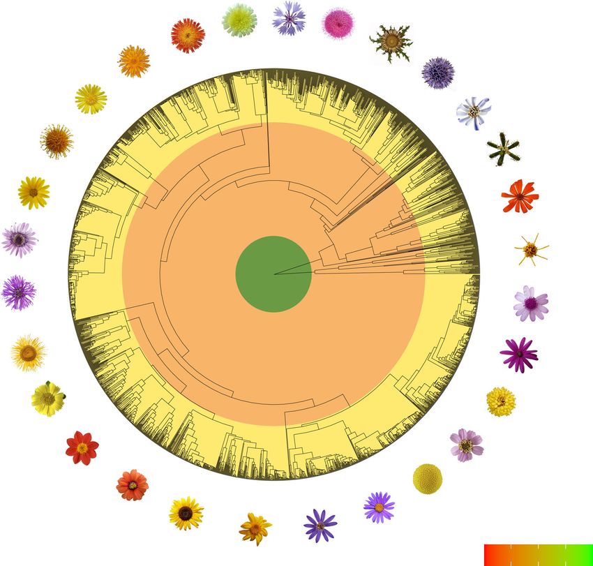
Fig. 1 Phylogenetic tree scaled to geological time of Asteraceae with 2723 sampled tips. Asteraceae is one of the most species-rich families of flowering
plants with more than 23,000 species. The number of non-sampled (missing) species increases enormously towards the more derived and species-rich
lineages. For this reason, the sampling among clades is severely biased. Note that these rich and derived lineages evolved during the late Paleogene or early
Neogene. K Cretaceous, Pg Paleogene, Ng Neogene.
(Supplementary Fig. 4 and 5), thus indicate rather a global (i.e., variation model and for the grasses phylogeny the fixed rate
tree-wide) pattern than a lineage-specific effect. model without additional variation. The support of the uncor-
Interestingly, estimations of low diversification rates prior to related model over the two autocorrelated models (GMRF and
~35Mya are consistent with the scarcity of fossil forms assigned HSRMF), although the autocorrelated models were favored when
to both daisies (Supplementary Table 1) and grasses4,39. Similarly, using time-varying diversification rates without environmental
high diversification rates during or after the Oligocene are in line variables (Supplementary Fig. 8), could stem from the use of
with the high diversity of fossil remains assigned to these vague prior distribution which allows for more rate variation in
groups4,40. The Cenozoic ‘temporal hotspot’ of grassland diver- autocorrelated models21. However, regardless of the specific
sification (~30 Mya to ~15 Mya) based on daisies and grasses environmentally dependent diversification model, we inferred a
(calibration #1 and #2) phylogenetic trees—coincides with one of negative correlation between diversification rates and environ-
the most fundamental changes in global climate in the geologic mental CO2 (Supplementary Fig. 10). The resulting Bayes factors
record; a marked decline of atmospheric CO2 occurred during the for a negative correlation were decisive with values of 37,501 for
Oligocene (~34 Mya), reaching modern levels by the latest the fixed, UC and GMRF models and 49 for the HSMRF model
Oligocene41,42. This scenario marks the onset of a cooler and (Fig. 3). We also see the same agreement between the four
more modern world (Coolhouse state), identified by the earliest environmentally-dependent diversification models in our simu-
Cenozoic glaciations in Antarctica, and the consequent drop in lation study (Supplementary Fig. 20 and 21). Thus, if there is a
global paleo-temperatures43. clear signal of correlation between the environmental variable and
In line with the reconstructed climatic scenario, our analyses of diversification rates, then our analyses appear robust to modeling
correlation between diversification rates and CO2 or paleo- of the additional component of time-varying diversification rates.
temperature show very interesting results (Fig. 3 and Supple- This agreement can also be seen when all four environmentally-
mentary Fig. 10 and 11). Diversification rates inferred from both dependent diversification models show the same estimated
the daisy and grasses phylogenies support correlation to CO2 over diversification rates (Supplementary Figs. 14 and 15). When the
paleo-temperature (Supplementary Fig. 11). Surprisingly, the best signal is less clear, as for the paleo-temperature analyses, the four
fitting environmentally-dependent diversification model for the models disagree and range from significant positive to significant
daisy phylogeny was the uncorrelated lognormal (UCLN) negative correlation (Supplementary Fig. 10) and the estimated
NATURE COMMUNICATIONS | (2022)13:293 | https://doi.org/10.1038/s41467-021-27897-y | www.nature.com/naturecommunications 3ARTICLE NATURE COMMUNICATIONS | https://doi.org/10.1038/s41467-021-27897-y
a) b)
8
8
log(lineages)
6
6
Carduoideae (2491) Andropogon. (1024)
Helianthodae (5996) Paniceae (866)
4
Asterodae (9941) Bambusoideae (1023)
4
Cichorioideae (3235) Aristidoideae (240)
Danthonioideae (47)
Arundinoideae-Micrairoideae(191)
2
Gochnatioideae (53)
2
Wunderlochieae (42) Chloridoideae (1187)
Mutisioideae (427) Ehrharteae (46)
Barnadesioideae (22) Pooideae (2515)
0
0
80 60 40 20 0 60 50 40 30 20 10 0
Time Time
Fig. 2 Lineage-Through Time (LTT) plots of daisies and grasses. Solid gray lines represent LTT curves derived from time-calibrated phylogenetic trees of
a Asteraceae and b Poaceae (calibration scenario #1). Colored boxes depict the name and number of non-sampled (missing) species per clade that we
integrated in our empirical taxon sampling. The shape of LTT curves have demonstrated to be a convenient summary metric for diversification diagnostics,
particularly when diversification deviates from the expectation of constant rates81,82. However, the distribution of missing species might not be uniform—
as it is the case of these angiosperm families—and can severely impact on diversification-rate estimates. Our work shows that the most important increase
in diversification rate for both Asteraceae and Poaceae is completely unnoticeable using the LTT analysis, even when calibrated phylogenetic trees include
a large number of species.
diversification rates of the environmentally-dependent diversifi- early radiation of grasslands48,49. The role of cooling in the emer-
cation models also differ (Supplementary Figs. 14 and 15). gence of open-habitat grasses has been debated as the adaptation to
Finally, our results of correlation between environmental CO2 low temperatures became prominent in the more derived groups of
and diversification rates are also robust to the chosen epoch size grasses4,50. Grazing mammals also have been important compo-
(Supplementary Fig. 12). nents in the evolution of grasslands; grazers and grassland ecosys-
The negative correlation between diversification rates of these tems probably coevolved over millions of years51. Grazing increased
selected grassland families and atmospheric CO2 might not be species diversity according to experimental studies, as grazers pre-
surprising; atmospheric CO2—the main source of carbon for vent dominant plant species from monopolizing resources. Without
photosynthesis—serves as a fundamental substrate for plant grazing, tall, vegetatively reproducing plant species increase in cover
growth. The available experimental evidence shows that low and shade out short and sexually reproducing species52. Grazing
atmospheric CO2 limits plant performance44, although responses also affects the flux of nutrients by accelerating the conversion of
vary significantly between species. At a landscape scale, carbon plant nutrients from forms that are unavailable for plant uptake to
limitation and water stress due to lower atmospheric CO2 con- forms that can be readily used. Overall, grazing mammals have an
centrations (‘ecophysiological drought’), rather than water stress important role in the diversity of present-day natural grasslands
due to lower precipitation (‘climatic drought’), cause changes in and we assume they might have done so during their early radia-
vegetation structure45. During the Last Glacial Maximum (LGM; tion. However, the explosive radiation of true hypsodonts may have
~21,000 years ago), for example, atmospheric CO2 was at its lowest negatively impacted grasslands’ distribution and diversity (see
concentration in the history of land plants (~180–200 ppm)46. below). Sorting out the relative importance of all these environ-
Models have predicted that the direct physiological impact of the of mental and biological competing forces from the hypothesized
low CO2 concentrations during the LGM drove the expansion of CO2-induced shift remains challenging.
grasslands and dry shrublands at the expense of forest47 (Supple- We detected a short decrease in diversification rates for daisy and
mentary Fig. 2). Other modeling experiments indicate that low grass plant groups during the mid-Miocene, about 13–10 Mya
atmospheric CO2, in combination with increased aridity and (Figure 3a). The causal mechanism underlying remains to be eluci-
decreased temperatures, causes new xeric biomes to develop46. dated. However, we suspect that the dramatic radiation of hypsodont
Although our primary hypothesis is that a CO2-depleted atmo- grazers—such as horses—and other mixed feeder grazers may have
sphere played a role in the geographic expansion and diversification had an impact on grasslands3,53. Since the late Miocene (~10 Mya),
of grassland families from Oligocene times (~34 Mya), other however, the more recent expansion of C4 grass lineages11 may have
environmental and biological variables could have also been contributed to the increased diversification rates in these groups.
involved. In particular, the decreasing temperatures, increasing Plants using the C4 photosynthetic pathway have anatomical and
aridity, and increasing seasonality of temperature and/or pre- biochemical adaptations for concentrating CO2 within leaf cells prior
cipitation of the late Cenozoic have been traditionally linked to the to photosynthesis, which may lead to a selective advantage over C3
4 NATURE COMMUNICATIONS | (2022)13:293 | https://doi.org/10.1038/s41467-021-27897-y | www.nature.com/naturecommunicationsNATURE COMMUNICATIONS | https://doi.org/10.1038/s41467-021-27897-y ARTICLE
a) b)
Daisies Grasses
PP(β < 0) PP(β < 0)
0.4
Model
CO 2 GMRF 1 1
Daisies HSMRF 0.98 1
Grasses UC 1 1
fixed 1 1
0.3
CO2
800
atmospheric CO2 (ppm)
net−diversification rate
700
0.2
600
500
−0.015 −0.010 −0.005 0.000 0.005 −0.008 −0.006 −0.004 −0.002 0.000
PP(β < 0) PP(β < 0)
0.1
400
0.49 0.26
0.05 0.09
1 1
Paleo-temperature
1 1
300
0.0
Pleistocene
Oligocene
Pliocene
Miocene
Eocene
Paleogene Neogene Q.
−1.0 −0.5 0.0 0.5 1.0 −0.4 −0.2 0.0 0.2 0.4 0.6 0.8
50
40
30
20
10
0
beta speciation beta speciation
Age (Mya)
Fig. 3 Estimating diversification rates and correlation to CO2 and paleo-temperature. a Diversification rates through time of daisies (yellow) and grasses
(green)—calibration scenario #1—for the last 50 Mya. Dotted line represents atmospheric CO2 fluctuations (22); note that the Oligocene steep decrease
mirrors the onset of the increase in diversification of daisies and grasses. Gray arrow indicates a period (13–10 Mya) of lower diversification rates probably
linked either with a brief increase in CO2 (not represented in the dotted smoothed curve) or the explosive radiation of hypsodont grazers (e.g., horses) and
other mixed feeder grazers3 who may have had a tremendous impact on grasslands through their effects on plant populations and community composition.
b The correlation factor (β) between diversification rates and CO2 concentrations for daisies and grasses is significantly negative (posterior probability of
1.0 for all models except the HSRMF, which has a posterior probability of 0.98; Bayes factors of 37,501 and 49 respectively). The support for a negative
correlation between paleo-temperature and diversification rates is ambiguous; the UC and fixed models show significant support (posterior probability of
1.0, Bayes factor of 37,501) while the autocorrelated models show no support (posterior probability between 0.05 and 0.095, Bayes factors supporting a
positive correlation of 1.04 and 17.86 for the daisy dataset and 2.85 and 9.75 for the grasses dataset for the GMRF and HSMRF models respectively). Note
that the correlation factor β does not follow the same scale as common correlation coefficients (which are between −1 and 1) but instead represents the
factor by which to transform the environmental variable into diversification rates (see “Methods”).
plants under conditions of low atmospheric CO2. Although the Methods
evolutionary origin of C4 photosynthesis in grasses most likely Taxonomic representativeness in grasslands. To quantify the taxonomic repre-
sentativeness of vascular-plant families found in open-habitat landscapes (Supple-
occurred early in the Cenozoic32, their expansion and ecological mentary Fig. 1), we selected seven distantly distributed eco-regions dominated by
dominance may have taken place during the last 10 Mya, by the late grasslands from the World Wide Fund for Nature58. Using the coordinate boundaries
Miocene in warmer and fire-prone landscapes of the world54. Like- of each of the selected eco-regions, we extracted the vascular plant taxa (=Tracheo-
wise, the evolution of hyper-diverse Asteraceae lineages (e.g., phyta) using the R ‘rgbif:Interface to the Global ‘Biodiversity’ Information Facility API’
Senecio)55 have also contributed to the increasing rates of diversifi- package59 with the option ‘hasGeospatialIssue=FALSE’, that includes only records
without spatial issues (e.g., invalid coordinates, country coordinate mismatch). Plant
cation since the last 10 Mya. Our evidence also supports the notion families were sorted according to the number of species, removing duplicated species.
that the ongoing rise of atmospheric CO2 will likely alter vegetation
distributions through differential effects on C3 and C4 plant types. In
Palaeobotanical analysis. Asteraceae and Poaceae have a fairly similar fossil record;
fact, modeling future distributions predicts the near-complete eradi- their oldest findings are known from the Late Cretaceous—which mainly comprise
cation of C4 species across the globe for the next 50 years56; this microscopic remains (that is, phytoliths60 or pollen grains61)—whereas the first indis-
implies that about half of the species in the grass family will be putable macroscopic Asteraceae and Poaceae fossils are first known from the
extinct. In summary, our study reveals episodic shifts in diversifica- Eocene62,63, with a substantial increase of diversity since the Oligocene/Miocene. While
the fossil record of Poaceae has been fully revised4,64,65, the fossil record of Asteraceae
tion rates of grasses and daises which are correlated with changes in has not been as carefully reviewed. We compiled published pollen and macroscopic
atmospheric CO2 (Fig. 3a); these insights are made possible by the fossil data for Asteraceae including all fossil species assigned to Asteraceae (Supple-
development of our Bayesian phylogenetic approach which combines mentary Table 1). The earliest record of the Asteroideae (the clade that includes the
the episodic birth–death process18–21 with environmentally- most common open-habitat daisy tribes) occurs since the Late Oligocene of New
Zealand but in very low frequencies. Fossils refer to this subfamily increased in
dependent diversification rates22–24,26 and empirical taxon abundance and diversity during the Miocene and Pliocene. Pollen referred to Artemisia,
sampling15,16,57. Our environmentally dependent and episodic in particular, did not become abundant until the Middle-Late Miocene with several
birth–death diversification model provides an approach for exploring reports from central Europe, Asia and North America. Pre-Miocene findings need
the evolution of hyper-diverse groups of plants and animals in the further verification. Overall, the Late Oligocene and in particular the Miocene witnessed
the major step in the diversification of Asteraceae; ca. 80% of the fossil species recorded
context of historical environmental changes. have been assigned to this time interval.
NATURE COMMUNICATIONS | (2022)13:293 | https://doi.org/10.1038/s41467-021-27897-y | www.nature.com/naturecommunications 5ARTICLE NATURE COMMUNICATIONS | https://doi.org/10.1038/s41467-021-27897-y
Divergence-time estimation. To construct the Asteraceae supertree (2723 tips), we Empirical taxon-sampling model. Here we develop an empirical taxon-sampling
first inferred a backbone chronogram using 14 plastid DNA regions from 54 species, model that uses taxonomic information on the membership of unsampled species
including representatives of all 13 subfamilies, with an additional four species of to clades and speciation times of unsampled species, which is an extension to the
Calyceraceae used as outgroup taxa (Supplementary Table 2). Sequences were compiled work by Höhna et al15,16 and similar to the approach used by Stadler and Bokma57.
from GenBank and each region was aligned separately using MAFFT66 with the options The main difference of our approach and the approach by Stadler and Bokma57 is
maxiterate 1000 and localpair. Two fossil constraints were applied: (i) a macrofossil that their model uses a constant-rate birth–death process (compared to our epi-
(capitulum) and associated pollen (Raiguenrayun cura + Mutisiapollis telleriae) from sodic birth–death process). Additionally, Stadler and Bokma57 derive the density of
the Eocene (45.6 Mya) to calibrate the non-Barnadesioideae Asteraceae clade63 and; (ii) the missing species using a random probability s of an edge being sampled, which
the fossil-pollen species Tubulifloridites lilliei type A from the late Cretaceous (72.1 differs from our approach where we integrate over the time of the missing spe-
Mya)61 to calibrate the crown Asteraceae (considering T. lilliei as a stem group, see ciation event. Nevertheless, at least for the constant-rate birth–death process, both
Huang et al.67 for further discussion). Divergence-time estimates and phylogenetic approaches arrive at the same final likelihood function.
relationships were inferred using RevBayes17. For the aligned molecular sequences we We include information on the missing speciation events by integrating over
assume a general-time reversible substitution model with gamma-distributed rate var- the known interval when these speciation events must have occurred (that is,
iation among sites (GTR+Γ), an UCLN prior on substitution-rate variation across between the stem age tc of the MRCA of the clade and the present, Figure 4). This
branches (UCLN relaxed clock), and a birth–death prior model on the distribution on integral of the probability density of a speciation event is exactly the same as one
node ages/tree topologies. A densely sampled phylogeny is crucial to identify shifts in minus the cumulative distribution function of a speciation event16,
diversification rates. Therefore, we constructed a supertree by inserting eleven individual
1 PðNðTÞ>0jNðt c Þ ¼ 1Þ expðrðt c ; TÞÞ
sub-trees —representing all subfamilies of the Asteraceae except those less diverse or Fðt c jNðt 1 Þ ¼ 1; t 1 ≤ t ≤ TÞ ¼ 1 ; ð2Þ
monotypic clades (that is, Gymnarrhenoideae, Corymbioideae, Hecastocleidoideae, 1 PðNðTÞ>0jNðt 1 Þ ¼ 1Þ expðrðt 1 ; TÞÞ
Pertyoideae)—into the calibrated backbone chronogram. This method follows a pre- where t1 is the age of the root. The probability of survival is given by:
vious study that constructed a supertree of grasses using the same approach11. Each of
the eleven clades of Asteraceae was built using their own set of markers and the same PðNðTÞ > 0jNðt c Þ ¼ 1Þ
phylogenetic approach as the one used to infer the backbone tree (Supplementary i1 ! k
!1
k μi ∑ ðμj λj Þðxjþ1 xj Þ ρ 1 i¼c
∑ ðμ λi Þðxiþ1 xi Þ
Table 2). Sequence data for each of the eleven trees and their respective outgroup taxa ¼ 1þ ∑ ´ e j¼c ´ ðeðμi λi Þðxiþ1 xi Þ 1Þ ´e i
i¼c μi λi ρ
were collected from Genbank using the NCBIminer tool68. The estimated ages of the
nodes given by the backbone analysis were used to constrain the age of each of the ð3Þ
eleven sub-trees (Supplementary Table 2). Divergence-time estimates and phylogenetic
relationships for each of the eleven sub-clades were estimated using RevBayes as where k ¼ jXj. Let us define n as the number of sampled species, m as the total
number of species in the study group, K as the set of missing species per clade and
described above. The eleven trees were grafted onto the backbone tree using the
function ‘paste.tree’ from the phytools R package69. We used ggtree R package70 to plot jKj the number of clades with missing species. Additionally, we define ci as the
time of most recent common ancestor of the ith clade. Then, the joint probability
the circle phylogenetic tree of Figure 1 and phytools69 to include the concentric geo-
density of the sampled reconstructed tree and the empirically informed missing
logical scale. The supertree of the grass family (3,595 taxa) was obtained from Spriggs
et al.11 (Supplementary Table 3). They inferred two chronograms using two different speciation times is
calibration scenarios, that is, a younger scenario (#1) calibrated using an Eocene f ðΨ; KjNðt 1 ¼ 0Þ ¼ 2; Sð2; t 1 ¼ 0; TÞÞ ¼ f ðΨjNðt 1 ¼ 0Þ ¼ 2; Sð2; t 1 ¼ 0; TÞÞ
megafossil62 and an older scenario (#2) calibrated using Cretaceous phytoliths60. We
ðm 1Þ! Y 1
jKj
ran our diversification analyses using these two chronograms. k
´ 1 FðtjNðci Þ ¼ 1; ci ≤ t ≤ TÞ i :
ðn 1Þ! i¼1 ki !
Inferring changes in diversification rate through time. Our species- ð4Þ
diversification model is based on the reconstructed evolutionary process described
by Nee et al.12 and more specifically on the episodic birth–death process18–21. We
assume that each lineage gives birth to another species with rate λ (cladogenetic Prior models on diversification rates. Our model assumes that speciation and
speciation events) and dies with rate μ (extinction event; see Fig. 4). We model extinction rates are piecewise constant but can be different for different time
diversification rates (i.e., speciation and extinction rates) as constant within an intervals (Fig. 4). Thus, we divide time into equal-length intervals (e.g., Δt = 1).
interval but independent between intervals, where intervals are demarcated by Following Magee et al.21, we specify prior distributions on the log-transformed
instantaneous rate-shift events, and equal among contemporaneous lineages. We speciation rates (ln ðλi Þ) and extinction rates (ln ðμi Þ) because the rates are only
denote the vector of speciation rates Λ = {λ1, …, λk} and extinction rates defined for positive numbers and our prior distributions are defined for all real
M = {μ1, …, μk} where λi and μi are the (constant) speciation and extinction rates in numbers. We apply and compare three different prior models: (i) an UCLN prior
interval i. Additionally, we use the taxon-sampling fraction at the present denoted distribution, (ii) a GMRF prior21, and (iii) a HMRF prior21. The first prior dis-
by ρ15,16. Following the notation of May et al.20, we construct a unique vector, X, tribution specifies temporally uncorrelated speciation and extinction rates, whereas
that contains all divergence times and rate-shift event times sorted in increasing the second and third prior distributions are autocorrelated prior models. The
order. It is convenient for notation to expand the vectors for all the other para- assumption of autocorrelated rates might make more sense biologically (an interval
meters so that they have the same number of elements k ¼ jXj. Let Ψ denote an of high speciation rates is likely to be followed by another interval with high
inferred tree relating n species, comprising a tree topology, τ, and the set of speciation) but also improves our ability to estimate parameters21. Nevertheless,
branching times, T. We use the notation S(2, t1 = 0, T) to represent the survival of our inclusion of both uncorrelated and autocorrelated prior distributions allows for
two lineages in the interval [t1, T], which is the condition we enforce on the testing whether an uncorrelated or autocorrelated model is preferred.
reconstructed evolutionary process. Transforming Equation (A4) in May et al.20 to The prior distribution on the speciation rates λi and extinction rates μi are set in
our model yields the probability density of a reconstructed tree as: exactly the same form in our models with their respective hyperprior parameters.
Thus, for the sake of simplicity, we omit the prior distribution on the extinction
rates here in the text. Our first prior distribution, the UCLN distributed prior,
f ðΨjNðt 1 ¼ 0Þ ¼ 2; Sð2; t 1 ¼ 0; TÞÞ
specifies the same prior probability for each speciation rate λi,
2n1
¼ ln ðλi Þ Normal ðm; σÞ: ð5Þ
n!
i1 ! !2
∑ ðμj λj Þðxjþ1 xj Þ
k
μi k ρ 1 i¼0
∑ ðμ λi Þðxiþ1 xi Þ Thus, each speciation rate is independent and identically distributed.
´ 1þ ∑ ´ ej¼0 ´ eðμi λi Þðxiþ1 xi Þ 1 ´e i
i¼0 μi λi ρ Our second prior distribution, the GMRF prior, models rates in an
k !2 autocorrelated form analogous to a discretized Brownian motion. That is, we
log ðρÞ ∑ ðμj λj Þðxjþ1 xj Þ assume that diversification rates λ(t) and μ(t) are autocorrelated and the rates in the
´ e j¼0
next time interval will be centered at the rates in the current time interval,
" !
Y ∑ ðμj λj Þðxjþ1 xj Þ ln ðλi Þ Normal ðln ðλi1 Þ; σ λ Þ: ð6Þ
l1
k μl
´ λi ´ 1 þ ∑ ´ ej¼0 ´ eðμl λl Þðxlþ1 xl Þ 1
μ l λl
i2IT
l¼i
The standard deviation σ regulates the amount of change between each time
!2 #
ρ 1 l¼i
k
∑ ðμl λl Þðxlþ1 xl Þ
k
log ðρÞ ∑ ðμj λj Þðxjþ1 xj Þ
interval.
´e ´e j¼i
: Our third prior distribution, the HSMRF prior, is very similar to the GMRF but
ρ
additionally allows for the variance to change between time intervals,
ð1Þ
γi halfCauchy ð0; 1Þ ð7Þ
2n1
The first term, corresponds to the combinatorial constant for the number of
n! ln ðλi Þ Normal ðln ðλi1 Þ; σγi Þ: ð8Þ
labeled histories18, the second term corresponds to the condition of two initial
lineage at the root of the phylogeny surviving until the present, and the third term The HSMRF prior model is more adaptive than the GMRF; it allows for more
corresponds to the product of all speciation events and the new lineages surviving extreme jumps between intervals while favoring/smoothing more constant-rate
until the present. trajectories if there is no evidence for rate changes21.
6 NATURE COMMUNICATIONS | (2022)13:293 | https://doi.org/10.1038/s41467-021-27897-y | www.nature.com/naturecommunicationsNATURE COMMUNICATIONS | https://doi.org/10.1038/s41467-021-27897-y ARTICLE
a) Diversification rates through times d) Sampled phylogeny with missing species
Rate-shift event
1.5 2 missing species
1.0
0.5
1 missing species
0.0
20
30
10
0
time before present
b) Complete phylogeny
Extinction event
Speciation event
e) Distribution function of missing speciation event
F(t)
1.0
time of missing
speciation event
c) Reconstructed phylogeny
0.0
time before present
Fig. 4 Cartoon of the birth–death process with rate-shift events and empirical taxon sampling. a Depiction of the speciation (purple lines) and extinction
(red lines) rates through time. Here we assume that speciation and extinction rates are episodically constant, that is, diversification rates shift instantly and
only at the beginning of an episode. Each episode lasts five time units in this example. b A realization (complete phylogeny) of the birth–death process.
Lineages that have no extant or sampled descendant are shown as dashed lines and surviving lineages are shown as solid lines. c Reconstructed phylogeny
corresponding exactly to the one shown in B with the extinct lineages pruned away. Thus, plot c depicts the “observed” phylogeny from which the
speciation times are retrieved. d Sampled phylogeny with gray boxes depicting named clades with known number of missing species. The phylogeny is the
same as in c with fewer taxa. e Distribution function of the time of the missing speciation event. The missing speciation event could have occurred any time
between the crown age of the named clade and the present time (gray box). The distribution function is integrated over and hence the uncertainty of the
missing speciation event accounted for.
These three prior models of diversification rates provide the null models of our We applied this original environmentally-dependent diversification model and
analyses as they do not assume any dependence to an environmental variable. We three environmentally-dependent diversification models described in this work.
use these models first to estimate diversification rates through time before testing for The original environmentally-dependent diversification model of Condamine
a correlation of the speciation or extinction rate to an environmental variable (e.g., et al.22 does not accommodate diversification-rate variation that is independent of
atmospheric CO2 or paleo-temperature). Magee et al.21 found that 100 epochs the environmental variable. Instead, our three environmentally-dependent
perform well for autocorrelated models. Since we do not know how many bins (i.e., diversification models build on our diversification-rate prior models which allow
epochs) should be used for the episodic birth–death process, we test various numbers for rate variation through time (see above). Thus, our environmentally-dependent
of equal-sized epochs (4, 10, 20, 50, 100, and 200, Supplementary Figure 7). We show diversification models will collapse to the episodic birth–death model if rates of
both the median posterior diversification rates (Supplementary Fig. 6) as well as diversification and atmospheric CO2 are uncorrelated and hence inherently allows
select the best fitting model based on the number of epochs (Supplementary Fig. 8). for diversification rate variation. The linkage of environmental variable and
diversification rates without allowing for independent diversification rate variation
might provide spurious results, as has been noticed for trait evolution72 and state-
Correlation between speciation and extinction rate to CO2. Previously, Con- dependent diversification rates73. We explore this potential of misattribution of
damine et al.22 introduced an environmentally-dependent diversification model. In diversification rate variation to the environmental variable in our model selection
their model, diversification rates are correlated with an environmental procedure and simulation study (see below).
As before, we omit the description of the extinction rates in the text for the sake
variable22–27. For example, the speciation rate can be modeled as λðtÞ ¼ of notational simplicity. Both speciation and extinction rates are model exactly in
λ0 eβ ´ CO2 ðtÞ (see Box 1 in Condamine et al.22), which is equivalent to the same way with their corresponding set of hyperparameters (e.g., see the
ln ðλðtÞÞ ¼ ln ðλ0 Þ þ β ´ CO2 ðtÞ. Since we are using the episodic birth–death process Supplementary Tables 4–7). Our first environmentally-dependent diversification
which has piecewise-constant diversification rates, we modify the original model has a fixed linkage between the diversification rate variation and variation in
continuous-time environmentally-dependent diversification model to the environmental variable;
ln ðλi Þ ¼ ln ðλ0 Þ þ β ´ CO2;i , which is equivalent to and more conveniently written
as ln ðλi Þ ¼ ln ðλi1 Þ þ β ´ ΔCO2;i where ΔCO2,i = CO2,i − CO2,i−1. Note that we λ0 Uniform ð0; 100Þ ð9Þ
only use the so-called exponential dependency and not the linear dependency24
because the linear dependency can result in negative rates which are mathemati-
cally and biologically impossible71. ln ðλi Þ ¼ ln ðλi1 Þ þ βλ ´ ΔCO2 : ð10Þ
NATURE COMMUNICATIONS | (2022)13:293 | https://doi.org/10.1038/s41467-021-27897-y | www.nature.com/naturecommunications 7ARTICLE NATURE COMMUNICATIONS | https://doi.org/10.1038/s41467-021-27897-y
This model does not have a counterpart in the above diversification rate priors, but MCMC run with 2000 iteration and on average 1374 moves per iteration (i.e., the
is included as a comparison to the work Condamine et al.22. runs being equivalent to standard single-move-per-iteration software with
Our second environmentally-dependent diversification model adds UCLN 2,748,000 iterations).
variation on top of the variation in the environmental variable; We tested the support for the environmental correlation using Bayes factors
computed from the posterior odds. Our prior probability for the correlation factor β
λ0 Uniform ð0; 100Þ ð11Þ was symmetric and centered at zero, that is, we specified exactly a probability of 0.5
that β < 0 and β > 0. Thus, the prior probability ratio of Pðβ0Þ ¼ 1:0 Then, to compute
ln ð^λi Þ ¼ ln ð^λi1 Þ þ βλ ´ ΔCO2 ð12Þ
the Bayes factor for in support of a negative correlation is simply the number of
MCMC samples with β < 0 divided over the total number of MCMC samples.
ϵi Normal ð0; σÞ ð13Þ We did not compute marginal likelihoods for the two different sampling
schemes; the uniform taxon sampling and the empirical taxon sampling. Empirical
ln ðλi Þ ¼ ln ð^λi Þ þ ϵi : ð14Þ taxon sampling uses additional data, the age ranges of the missing speciation
events, and two analyses with different data cannot be compared using traditional
Thus, this model collapses to the above UCLN model if there is no correlation model selection. Instead, we performed a simulation study to show the robustness
between the environmental variable and diversification rates (β = 0). Importantly, of our parameter estimates under empirical taxon sampling and the resulting bias if
the difference in the variation of the diversification rates and environmental wrongly uniform taxon sampling was assumed.
variable is independent in each epoch, contributed by the variable ϵi. The
environmental-dependent part of the diversification rates ^λi is equivalent to the
fixed environmentally-dependent diversification model. Simulation study. We performed two sets of simulations; focusing (a) on the
Our third environmentally dependent diversification model adds correlated environmentally-correlated diversification model, and (b) the incomplete taxon
lognormal variation on top of the fixed environmentally-dependent diversification same scheme. First, we simulated phylogenies under the UCLN and GMRF
mode; environmentally-correlated diversification model using the R package TESS78,79.
We set the diversification rate variation to σ = {0, 0.02, 0.04} and correlation factor
λ0 Uniform ð0; 100Þ ð15Þ to β = {0, −0.005, −0.01}. Thus, our simulations included the constant-rate
birth–death process (when σ = 0 and β = 0), time-varying but environmentally
ln ðλi Þ Normal ðln ðλi1 Þ þ βλ ´ ΔCO2 Þ; σÞ: ð16Þ independent diversification rates (when σ > 0 and β = 0), the fixed
environmentally-dependent diversification model (when σ = 0 and β ≠ 0), and the
This model an extension of the above GMRF model and collapses to it if there is no time-varying and environmentally-dependent diversification model (when σ > 0
correlation between the environmental variable and diversification rates (β = 0). As and β ≠ 0). For each setting, we simulated ten diversification rate trajectories
the GMRF model is a discretized Brownian motion model, this environmentally- (Fig. S16 and S17) and trees (Fig. S18 and S19). We analyzed each simulated tree
dependent extension can be considered as a Brownian motion with trend model, under the same four environmentally dependent diversification model as in our
where the trend is predicted by the environmental variable. Instead of writing this empirical analysis (see above).
model with a separate environmentally-dependent part ^λi and autocorrelated part Second, we simulated phylogenetic trees under empirical taxon sampling to
ϵi, we directly use the combined environmentally-dependent and independent rate validate the correctness of our model derivation. Unfortunately, simulation of
variation as the mean for the next time interval. Nevertheless, we want to empirical taxon sampling is not straight forward. We circumvented the problem by
emphasize this equivalence to bridge the connection to the UCLN model above. randomly adding the missing species to the daisy phylogenetic tree, then drawing
Finally, our fourth environmentally-dependent diversification model extends the new divergence times under (a) a constant-rate birth–death process, and (b) a
above HSRMF to allow for diversification rates predicted by the environmental variable; time-varying episodic birth–death process with rates taken from the empirical
estimates. Then, we pruned the additional species to mimic empirical taxon
λ0 Uniform ð0; 100Þ ð17Þ
sampling. The simulations under the constant-rate birth–death process provide
information about falsely inferring diversification rate variation (false positives)
γi halfCauchy ð0; 1Þ ð18Þ and the simulations under the time-varying episodic birth–death process provide
information about the power to correctly inferring diversification rate variation
ln ðλi Þ Normal ðln ðλi1 Þ þ βλ ´ ΔCO2 Þ; σγi Þ: ð19Þ (power analysis). We simulated 100 trees under each setting and analyzed each tree
using the GMRF prior model with both empirical and uniform taxon sampling.
This model follows the same extension as the environmentally-dependent GMRF
The MCMC inference settings were identical to the empirical analyses.
model with local adaptability of the rate variation through the parameter γi, as before
for the HSMRF.
In all our four models, we denote the correlation factor by β. If β > 0 then there Reporting summary. Further information on research design is available in the Nature
is a positive correlation between the speciation rate and CO2, that is, if the CO2 Research Reporting Summary linked to this article.
increases then the speciation rate will also increases. By contrast, if β < 0 then there
is a negative correlation between the speciation rate and CO2, that is, if the CO2
concentration increases then the speciation rate will decrease. Finally, if β = 0 then Data availability
there is no correlation and our environmentally-dependent diversification model The authors declare that all data supporting the findings of our study are available within
collapses to corresponding episodic birth–death model. the article and its supplementary information files or upon request to the authors. Time-
All four models have the same parameter for the initial speciation rate λ0 with a calibrated phylogenies from grasses and daisies used in the present study are deposited at
uniform prior distribution between 0 and 100. The models are constructed in https://doi.org/10.5061/dryad.74b5d and Supplementary Data 1, respectively.
increasing complexity and all three models can collapse either to the fixed
environmentally-dependent diversification model or to their environmentally Code availability
independent episodic birth–death process. Both models, the episodic birth–death process and the environmentally-dependent
diversification model, are implemented in the Bayesian phylogenetics software
Environmental data. In our analyses we tested for correlation between two RevBayes version 1.1.117. Moreover, the implementation is not restricted to the models
environmental factors: CO2 and temperature. The concentration of atmospheric we introduce here because RevBayes is built on the principle of probabilistic graphical
CO2 throughout the Cenozoic were compiled by Beerling & Royer41 using ter- models80. The graphical model approach provides full flexibility to extend or modify the
restrial and marine proxies. An updated dataset was provided by Dr. Dana Royer. current analyses to other models and assumption, for example, testing for correlation to
Paleo-temperature fluctuations come from Zachos et al.74. Raw data were extracted multiple environmental variables. RevBayes is open-source and freely available from
from ftp://ftp.ncdc.noaa.gov/pub/data/paleo/. https://revbayes.github.io/. The analysis from this paper are described in detail in several
Analogous to our tests about the number of epochs for the diversification rate tutorials available at https://revbayes.github.io/tutorials/, specifically the tutorials https://
analyses, we computed the arithmetic mean for the environmental variable for 1-, revbayes.github.io/tutorials/divrate/ebd.html, https://revbayes.github.io/tutorials/divrate/
2- and 5-million year intervals. We both estimated the correlation between the env.html and https://revbayes.github.io/tutorials/divrate/sampling.html.
environmental variable and diversification rates for each interval size and
performed model selection using Bayes factors.
Received: 9 June 2017; Accepted: 13 December 2021;
Model selection. We performed three sets of empirical diversification rate analyses
for each dataset. We estimated the diversification rates over time using three dif-
ferent models, we estimated the environmentally-dependent diversification rates
using four different models, and we applied two different taxon-sampling schemes.
For the first two sets of analyses we performed standard model selection in a
Bayesian framework using Bayes factors75. Thus, we computed the marginal References
likelihood for each model using stepping-stone sampling76 as implemented in 1. Vitousek, P. M. Grassland ecology: complexity of nutrient constraints. Nat.
RevBayes77. We run 128 stepping stones with each stone comprising of its own Plants 1, 1–2 (2015).
8 NATURE COMMUNICATIONS | (2022)13:293 | https://doi.org/10.1038/s41467-021-27897-y | www.nature.com/naturecommunicationsNATURE COMMUNICATIONS | https://doi.org/10.1038/s41467-021-27897-y ARTICLE
2. Sala, O. E. et al. Global biodiversity scenarios for the year 2100. Science 287, 33. Hackel, J. et al. Grass diversification in madagascar: in situ radiation of two
1770–1774 (2000). large c3 shade clades and support for a miocene to pliocene origin of c4 grassy
3. Janis, C. M., Damuth, J. & Theodor, J. M. Miocene ungulates and terrestrial biomes. J. Biogeogr. 45, 750–761 (2018).
primary productivity: where have all the browsers gone? Proc. Natl Acad. Sci. 34. Mandel, J. R. et al. A fully resolved backbone phylogeny reveals numerous
USA 97, 7899–7904 (2000). dispersals and explosive diversifications throughout the history of asteraceae.
4. Strömberg, C. A. E. Evolution of grasses and grassland ecosystems. Ann. Rev. Proc. Natl Acad. Sci. USA 116, 14083–14088 (2019).
Earth Planet. Sci. 39, 517–544 (2011). 35. Pennell, M. W. et al. geiger v2. 0: an expanded suite of methods for fitting
5. Hill, R., Truswell, E.M., McLoughlin, S., & Dettmann, M. E. The evolution of macroevolutionary models to phylogenetic trees. Bioinformatics 30,
the Australian flora: fossil evidence. In Flora of Australia: Volume 1, 2216–2218 (2014).
Introduction. Vol. i, 251–320 (CSIRO Publishing, 1999). 36. Panero, J. L. & Crozier, B. S. Macroevolutionary dynamics in the early
6. Palazzesi, L. & Barreda, V. Fossil pollen records reveal a late rise of open- diversification of asteraceae. Mol. Phylogenet. Evol. 99, 116–132 (2016).
habitat ecosystems in Patagonia. Nat. Commun. 3, 1–6 (2012). 37. Rabosky, D. L. et al. Bamm tools: an r package for the analysis of evolutionary
7. Pennington, R. T., Cronk, Q. C. B. & Richardson, J. A. Introduction and dynamics on phylogenetic trees. Methods Ecol. Evol. 5, 701–707 (2014).
synthesis: plant phylogeny and the origin of major biomes. Philos. Trans. R. 38. Alfaro, M. E. et al. Nine exceptional radiations plus high turnover explain
Soc. B Biol. Sci. 359, 1455–1464 (2004). species diversity in jawed vertebrates. Proc. Natl Acad. Sci. USA 106,
8. Davis, C. C., Webb, C. O., Wurdack, K. J., Jaramillo, C. A. & Donoghue, M. J. 13410–13414 (2009).
Explosive radiation of Malpighiales supports a mid-cretaceous origin of 39. Azevedo J. A .R. et al. On the Young Savannas in the Land of Ancient Forests.
modern tropical rain forests. Am. Nat. 165, E36–E65 (2005). In Neotropical Diversification: Patterns and Processes. Fascinating Life Sciences.
9. Couvreur, T., Forest, F. & Baker, W. J. Origin and global diversification (eds Rull V. & Carnaval A.) (Springer Cham, 2020).
patterns of tropical rain forests: inferences from a complete genus-level 40. Barreda, V., Palazzesi, L., Tellería, M. C., Katinas, L. & Crisci, J. V. Fossil
phylogeny of palms. BMC Biol. 9, 44 (2011). pollen indicates an explosive radiation of basal Asteracean lineages and allied
10. Richardson, J. E., Pennington, R. T., Pennington, T. D. & Hollingsworth, P. M. families during Oligocene and Miocene times in the Southern Hemisphere.
Rapid diversification of a species-rich genus of neotropical rain forest trees. Rev. Palaeobot. Palynol. 160, 102–110 (2010).
Science. 293, 2242–2245 (2001). 41. Beerling, D. J. & Royer, D. L. Convergent Cenozoic CO2 history. Nat. Geosci.
11. Spriggs, E. L., Christin, P.-A. & Edwards, E. J. C4 photosynthesis promoted 4, 418–420 (2011).
species diversification during the miocene grassland expansion. PLoS ONE 9, 42. Rae, J. W. B. et al. Atmospheric CO2 over the past 66 million years from
e105923 (2014). marine archives. Ann. Rev. Earth Planet. Sci. 49, 609–641 (2021).
12. Nee, S., May, R. M., Harvey, P. H., Trans, P. & Lond, R. S. The reconstructed 43. Westerhold, T. et al. An astronomically dated record of earthas climate
evolutionary process. Philos. Trans. R. Soc. B Biol. Sci. 344, 305–11 (1994). and its predictability over the last 66 million years. Science 369, 1383–1387
13. Yang, Z. & Rannala, B. Bayesian phylogenetic inference using DNA sequences: (2020).
a Markov Chain Monte Carlo Method. Mol. Biol. Evol. 14, 717–24 (1997). 44. Robinson, J. M. Speculations on carbon dioxide starvation, Late Tertiary
14. Cusimano, N. & Renner, S. S. Slowdowns in diversification rates from real evolution of stomatal regulation and floristic modernization. Plant Cell
phylogenies may not be real. Syst. Biol. 59, 458–464 (2010). Environ. 17, 345–354 (1994).
15. Höhna, S., Stadler, T., Ronquist, F. & Britton, T. Inferring speciation and 45. Crucifix, M., Betts, R. A. & Hewitt, C. D. Pre-industrial-potential and Last
extinction rates under different sampling schemes. Mol. Biol. Evol. 28, Glacial Maximum global vegetation simulated with a coupled climate-
2577–2589 (2011). biosphere model: diagnosis of bioclimatic relationships. Glob. Planet. Change.
16. Höhna, S. Likelihood inference of non-constant diversification rates with 45, 295–312 (2005).
incomplete taxon sampling. PLoS ONE 9, e84184 (2014). 46. Cowling, S. A. & Sykes, M. T. Physiological significance of low atmospheric
17. Höhna, S. et al. RevBayes: Bayesian phylogenetic inference using graphical CO2 for plant-climate interactions. Quat. Res. 52, 237–242 (1999).
models and an interactive model-specification language. Syst. Biol. 65, 47. Harrison, S. P. & Prentice, C. I. Climate and CO2 controls on global
726–736 (2016). vegetation distribution at the last glacial maximum: analysis based on
18. Stadler, T. Mammalian phylogeny reveals recent diversification rate shifts. palaeovegetation data, biome modelling and palaeoclimate simulations. Glob.
Proc. Natl Acad. Sci. USA 108, 6187–6192 (2011). Change Biol. 9, 983–1004 (2003).
19. Höhna, S. The time-dependent reconstructed evolutionary process with a key- 48. Webb, S. D. A history of savanna vertebrates in the new world. part i: North
role for mass-extinction events. J. Theor. Biol. 380, 321–331 (2015). America. Ann. Rev. Ecol. Syst. 8, 355–380 (1977).
20. May, M. R., Höhna, S. & Moore, B. R. A Bayesian approach for detecting the 49. Axelrod, D. I. Rise of the grassland biome, central north America. Bot. Rev. 51,
impact of mass-extinction events on molecular phylogenies when rates of 163–201 (1985).
lineage diversification may vary. Methods Ecol. Evol. 7, 947–959 (2016). 50. Edwards, E. J. & Smith, S. A. Phylogenetic analyses reveal the shady history of
21. Magee, A. F. et al. Locally adaptive Bayesian birth-death model successfully c4 grasses. Proc. Natl Acad. Sci. USA 107, 2532–2537 (2010).
detects slow and rapid rate shifts. PLoS Comput. Biol. 16, e1007999 (2020). 51. Blair, J., Nippert, J. & Briggs, J. Grassland ecology. In Ecology and the
22. Condamine, F. L., Rolland, J. & Morlon, H. Macroevolutionary perspectives to Environment, 389–423 (Springer, 2014).
environmental change. Ecol. Lett. 16, 72–85 (2013). 52. Belsky, A. J. Effects of grazing, competition, disturbance and fire on species
23. Morlon, H. et al. RPANDA: an R package for macroevolutionary analyses on composition and diversity in grassland communities. J. Veg. Sci. 3, 187–200
phylogenetic trees. Methods Ecol. Evol. 7, 589–597 (2016). (1992).
24. Lewitus, E. & Morlon, H. Detecting environment-dependent diversification 53. Jardine, P. E., Janis, C. M., Sahney, S. & Benton, M. J. Grit not grass:
from phylogenies: a simulation study and some empirical illustrations. Syst. concordant patterns of early origin of hypsodonty in great plains ungulates
Biol. 67, 576–593 (2018). and glires. Palaeogeogr. Palaeoclimatol. Palaeoecol. 365, 1–10 (2012).
25. Condamine, F. L., Rolland, J., Höhna, S., Sperling, F. A. H. & Sanmartín, I. 54. Scheiter, S. et al. Fire and fire-adapted vegetation promoted c4 expansion in
Testing the role of the Red Queen and Court Jester as drivers of the the late miocene. New Phytol. 195, 653–666 (2012).
macroevolution of Apollo butterflies. Syst. Biol. 67, 940–964 (2018). 55. Kandziora, M., Kadereit, J. W. & Gehrke, B. Dual colonization of the
26. Condamine, F. L., Rolland, J. & Morlon, H. Assessing the causes of palaearctic from different regions in the afrotropics by senecio. J. Biogeogr. 44,
diversification slowdowns: temperature-dependent and diversity-dependent 147–157 (2017).
models receive equivalent support. Ecol. Lett. 22, 1900–1912 (2019). 56. Forrestel, E. J. & Edwards, E. J. The grasslands future biogeography of c3 and
27. Meseguer, A. S., Antoine, P.-O., Fouquet, A., Delsuc, F. & Condamine, F. L. c4. In Grasslands and Climate Change. (eds Gibson, D. J. & Newman, J. A.)
The role of the Neotropics as a source of world tetrapod biodiversity. Glob. 234–252 (Cambridge University Press, 2019).
Ecol. Biogeogr. 29, 1565–1578 (2020). 57. Stadler, T. & Bokma, F. Estimating speciation and extinction rates for
28. Louca, S. & Pennell, M. W. Extant timetrees are consistent with a myriad of phylogenies of higher taxa. Syst. Biol. 62, 220–230 (2013).
diversification histories. Nature 580, 502–505 (2020). 58. Olson, D. M. et al. Terrestrial ecoregions of the world: a new map of life on
29. Legried, B. Terhorst, J. A class of identifiable birth-death models. Preprint at Earth. Bioscience. 51, 933–938 (2001).
bioRxiv https://doi.org/10.1101/2021.10.04.463015v2 (2021). 59. Scott Chamberlain. rgbif: interface to the global ‘biodiversity’ information
30. Helmstetter, A. J. et al. Pulled diversification rates, lineages-through-time plots facility ‘API’. R package version 0.7 (2014).
and modern macroevolutionary modelling. Syst. Biol. syab083 https://doi.org/ 60. Prasad, V. et al. Cretaceous origin of the rice tribe provides evidence for early
10.1093/sysbio/output (2021). diversification in Poaceae. Nat. Commun. 2, 480 (2011).
31. Morlon, H., Hartig, F. & Robin, S. Prior hypotheses or regularization allow 61. Barreda, V. D. et al. Early evolution of the angiosperm clade Asteraceae in
inference of diversification histories from extant timetrees. Preprint at bioRxiv the Cretaceous of Antarctica. Proc. Natl Acad. Sci. USA 112, 10989–10994
https://doi.org/10.1101/2020.07.03.185074v1 (2020). (2015).
32. Christin, P.-A. et al. Molecular dating, evolutionary rates, and the age of the 62. Crepet, W. L. & Feldman, G. D. The earliest remains of grasses in the fossil
grasses. Syst. Biol. 63, 153–165 (2014). record. Am. J. Bot. 78, 1010–1014 (1991).
NATURE COMMUNICATIONS | (2022)13:293 | https://doi.org/10.1038/s41467-021-27897-y | www.nature.com/naturecommunications 9You can also read