The GRAVITY young stellar object survey - Spatially resolved kinematics of hot hydrogen gas in the star-disk interaction region of T Tauri stars
←
→
Page content transcription
If your browser does not render page correctly, please read the page content below
A&A 669, A59 (2023)
                                                                                                                                                         Astronomy
https://doi.org/10.1051/0004-6361/202244675
                                                                                                                                                          &
© The Authors 2023
                                                                                                                                                         Astrophysics

                               The GRAVITY young stellar object survey
 IX. Spatially resolved kinematics of hot hydrogen gas in the star-disk interaction
                              region of T Tauri stars
      GRAVITY Collaboration: J. A. Wojtczak1 , L. Labadie1 , K. Perraut2 , B. Tessore2 , A. Soulain2 , V. Ganci1,5 ,
      J. Bouvier2 , C. Dougados2 , E. Alécian2 , H. Nowacki2 , G. Cozzo2,15 , W. Brandner3 , A. Caratti o Garatti3,6,7 ,
        P. Garcia9,10 , R. Garcia Lopez3,6,11 , J. Sanchez-Bermudez3,8 , A. Amorim9,12 , M. Benisty2 , J.-P. Berger2 ,
     G. Bourdarot4 , P. Caselli4 , Y. Clénet13 , P. T. de Zeeuw4,14 , R. Davies4 , A. Drescher4 , G. Duvert2 , A. Eckart1,5 ,
      F. Eisenhauer4 , F. Eupen1 , N. M. Förster-Schreiber4 , E. Gendron13 , S. Gillessen4 , S. Grant4 , R. Grellmann1 ,
        G. Heißel13 , Th. Henning3 , S. Hippler3 , M. Horrobin1 , Z. Hubert2 , L. Jocou2 , P. Kervella13 , S. Lacour13 ,
          V. Lapeyrère13 , J.-B. Le Bouquin2 , P. Léna13 , D. Lutz4 , F. Mang4 , T. Ott4 , T. Paumard13 , G. Perrin13 ,
           S. Scheithauer3 , J. Shangguan4 , T. Shimizu4 , S. Spezzano4 , O. Straub4 , C. Straubmeier1 , E. Sturm4 ,
                                     E. van Dishoeck4,14 , F. Vincent13 , and F. Widmann4
                                                             (Affiliations can be found after the references)

                                                         Received 3 August 2022 / Accepted 12 October 2022

                                                                                     ABSTRACT

     Context. Hot atomic hydrogen emission lines in pre-main sequence stars serve as tracers for physical processes in the innermost
     regions of circumstellar accretion disks, where the interaction between a star and disk is the dominant influence on the formation of
     infalls and outflows. In the highly magnetically active T Tauri stars, this interaction region is particularly shaped by the stellar magnetic
     field and the associated magnetosphere, covering the inner five stellar radii around the central star. Even for the closest T Tauri stars,
     a region as compact as this is only observed on the sky plane at sub-mas scales. To resolve it spatially, the capabilities of optical long
     baseline interferometry are required.
     Aims. We aim to spatially and spectrally resolve the Brγ hydrogen emission line with the methods of interferometry in order to exam-
     ine the kinematics of the hydrogen gas emission region in the inner accretion disk of a sample of solar-like young stellar objects. The
     goal is to identify trends and categories among the sources of our sample and to discuss whether or not they can be tied to different
     origin mechanisms associated with Brγ emission in T Tauri stars, chiefly and most prominently magnetospheric accretion.
     Methods. We observed a sample of seven T Tauri stars for the first time with VLTI GRAVITY, recording spectra and spectrally dis-
     persed interferometric quantities across the Brγ line at 2.16 µm in the near-infrared K-band. We used the visibilities and differential
     phases to extract the size of the Brγ emission region and the photocentre shifts on a channel-by-channel basis, probing the variation
     of spatial extent at different radial velocities. To assist in the interpretation, we also made use of radiative transfer models of magneto-
     spheric accretion to establish a baseline of expected interferometric signatures if accretion is the primary driver of Brγ emission.
     Results. From among our sample, we find that five of the seven T Tauri stars show an emission region with a half-flux radius in the
     four to seven stellar radii range that is broadly expected for magnetospheric truncation. Two of the five objects also show Brγ emission
     primarily originating from within the co-rotation radius, which is an important criterion for magnetospheric accretion. Two objects
     exhibit extended emission on a scale beyond 10 R∗ , one of them is even beyond the K-band continuum half-flux radius of 11.3 R∗ . The
     observed photocentre shifts across the line can be either similar to what is expected for disks in rotation or show patterns of higher
     complexity.
     Conclusions. Based on the observational findings and the comparison with the radiative transfer models, we find strong evidence to
     suggest that for the two weakest accretors in the sample, magnetospheric accretion is the primary driver of Brγ radiation. The results for
     the remaining sources imply either partial or strong contributions coming from additional, spatially extended emission components in
     the form of outflows, such as stellar or disk winds. We expect that in actively accreting T Tauri stars, these phenomena typically occur
     simultaneously on different spatial scales. Through more advanced modelling, interferometry will be a key factor in disentangling their
     distinct contributions to the total Brγ flux arising from the innermost disk regions.
     Key words. stars: formation – techniques: interferometric – techniques: high angular resolution – infrared: stars –
     accretion, accretion disks – stars: variables: T Tauri, Herbig Ae/Be

1. Introduction                                                                                 of great importance in providing insight into many aspects of
                                                                                                star formation. Active research into this topic is connected to a
Since the interplay between a young stellar object (YSO) and its                                variety of astrophysical concepts, ranging from high level mod-
circumstellar disk has a major influence on the different phases                                els of stellar evolution down to the environmental conditions in
of its development, the study of such a star-disk interaction is                                the cradles of planet formation and the mechanics that govern

                                                                                                                                                                          A59, page 1 of 40
                 Open Access article, published by EDP Sciences, under the terms of the Creative Commons Attribution License (https://creativecommons.org/licenses/by/4.0),
                                  which permits unrestricted use, distribution, and reproduction in any medium, provided the original work is properly cited.
                             This article is published in open access under the Subscribe-to-Open model. Subscribe to A&A to support open access publication.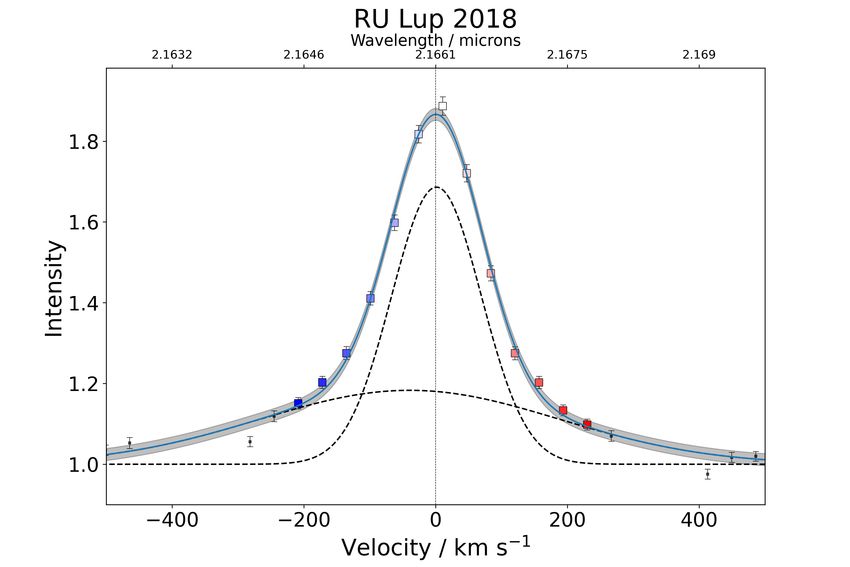
A&A 669, A59 (2023)

mass accretion during the pre-main sequence stage of a YSO.            (Ferreira 2013). For Herbig stars, a wind contribution in the Brγ
A number of ideas regarding the processes behind accretion             emission has been proposed in previous interferometric works
and ejection of matter in the inner disk have been extensively         (Garcia Lopez et al. 2015; Kurosawa et al. 2016). On the con-
explored in theoretical models and are relatively well established     trary, Brγ emission arising from a more compact region close to
on a conceptual level. However, the exact nature of the physi-         the star is considered, in particular in magnetically active T Tauri
cal interaction in the innermost circumstellar region inside 0.1 au    stars, to originate in the accretion columns located inside the
from the central star is still debated because the observational       magnetospheric truncation radius Rtr , at which point the ram
evidence for many of these concepts remains mostly indirect.           pressure of the infalling material is compensated for by the mag-
In this context, a distinction arises between intermediate-mass        netic pressure exerted perpendicular to the field lines (Bessolaz
Herbig stars and low-mass T Tauri stars. The latter has a lower        et al. 2008). A useful parameter to differentiate compact versus
effective temperature and weaker mass-accretion rates, but also        extended emission in the context of magnetospheric accretion
exhibits significant magnetic field strengths of 1–2 kG due their      can be the co-rotation radius Rco , which is the radius at which
convective nature (e.g. Johns-Krull 2007). This substantial dif-       the angular velocities of the gaseous disk and of the star equate
ference in the level of magnetic activity has given rise to the        (Bouvier 2013). Since the formation of stable funnels is only
paradigm of magnetospheric accretion. As a theory concern-             possible if the disk is truncated within the co-rotation radius
ing accretion in low-mass YSOs, it has attained preeminence            (Romanova & Owocki 2016), Brγ emission detected inside Rco
due to its ability to reconcile accretion properties with the pres-    indicates the probable presence of magnetospheric accretion
ence of stellar hot spots and the observations of hydrogen line        flows. Following Fig. 1, it is clear that the mechanisms involved
profiles (Camenzind 1990; Calvet & Hartmann 1992). It has              in the accretion process of matter in low-mass pre-main sequence
superseded the earlier theory of boundary layer accretion, which       stars are acting on a scale of a few (for the magnetic accretion)
is still thought to govern the processes of mass accretion in          to a few tens (in the case of winds) of stellar radii.
magnetically weak intermediate mass Herbig Ae/Be type YSOs                 Prior to the advent of NIR long baseline interferometry,
(Mendigutía 2020).                                                     observational evidence for the magnetospheric accretion sce-
    In the model of magnetospheric accretion, it is proposed that      nario has mainly been discussed in the context of high spectral
the inner gaseous disk is truncated by the strong stellar magnetic     resolution spectroscopy studies by Muzerolle et al. (1998), who
field because of the magnetic pressure exerted perpendicular to        have shown that the magnetospheric accretion model could pre-
the magnetic field lines threading the disk. Thus, a region of a       dict the Brγ profiles. The process of magnetospheric accretion
few stellar radii surrounding the star is formed where the disk        would influence the shape and strength of hydrogen emission
plane is almost completely evacuated from gas particles (Bouvier       lines, with a characteristic inverse P Cygni profile caused by
et al. 2007). Instead of further spiralling inwards, the gas parti-    infalling optically thick gas (e.g. Calvet & Hartmann 1992;
cles can only move freely along the field lines, which effectively     Edwards 1994; Petrov et al. 2014), typically observed at high
serve as funnels that channel the gas onto the star. As the gas        inclination of the system. Through theoretical simulations,
impacts the stellar surface at high latitudes, it creates heated       Kurosawa et al. (2011) investigated how the combination of
shock regions close to the poles (Hartmann et al. 2016).               the magnetospheric model with a (stellar-disk) wind model can
    Hydrogen emission lines serve as tracers for the kinemat-          qualitatively reproduce the observed profiles. However, with-
ics of the hot gas in the inner star-disk system. In particular the    out spatially resolving the star-disk interacting regions, such a
near-infrared (NIR) Brγ line at 2.16 µm, which is directly rel-        picture remains incomplete since such spectroscopic features
evant for this work, requires the gas to be at temperatures of         with their overall line shapes are not unique to magnetospheric
8000–10 000 K (Muzerolle et al. 1998; Tambovtseva et al. 2016)         accretion.
in order to produce strong emission. A heated gaseous disk in              With the advent of long baseline interferometry delivering
Keplerian rotation can, in principle, be the cause for the Brγ         sub-milliarcsecond resolution and the concomitant improvement
emission in YSOs, in particular for intermediate-mass Herbig           in the sensitivity of the technique, a larger reservoir of Brγ emit-
Ae/Be stars (Kraus et al. 2008). However, even in those cases,         ting T Tauri stars at a few hundred parsecs distance has become
theoretical considerations indicate that the total line-flux contri-   accessible. This has been exploited in the past in the works of
bution coming from the hot disk layers is faint compared to the        Eisner et al. (2010, 2014), who examined Brγ emission in a num-
contribution from outflows and infalls (see again Tambovtseva          ber of T Tauri stars with the Keck Interferometer, as well as in
et al. 2016). In T Tauri stars, with their much lower effective        recent pioneering studies with the Very Large Telescope Interfer-
temperatures and comparatively lower mass-accretion rates, the         ometer (VLTI) by GRAVITY Collaboration (2017b) for S CrA,
radiation field strength alone is insufficient to heat the gas disk    GRAVITY Collaboration (2020) for TW Hya, and Bouvier et al.
up to such temperatures at scales of 0.1 au (Natta 1993). It is then   (2020) for DoAr 44.
reasonable to assume that only specific heating mechanisms act-            In this paper, we report on observations made with GRAV-
ing much closer to the star in the accretion funnel flows or in        ITY (GRAVITY Collaboration 2017a), the second generation
the stellar-disk wind-launching regions result in the formation        beam combiner instrument of the VLTI, of a small sample of
of Brγ emission lines. Consequently, Brγ emission in T Tauri           seven accreting T Tauri stars. We aim to improve upon the results
stars is an excellent tracer of the processes associated with such     obtained in previous studies by combining the high angular and
gas-heating mechanisms, in particular for the magnetospheric           spectral resolution offered by GRAVITY to present spectrally
accretion model which is believed to play a central role in the        dispersed measurements of the Brγ emission region across the
evolution of low-mass pre-main sequence stars.                         sample, capable of identifying broader trends and categories
    Figure 1 illustrates how different possible mechanisms pro-        between the different objects. We contextualise our findings by
ducing Brγ emission are tied to different spatial scales. Brγ          drawing upon the latest results in radiative transfer modelling
emission coming from extended parts of the gaseous disk closer         of magnetospheric accretion in Brγ , deriving sets of synthetic
to the sublimation radius is likely to trace outflows in the form      observables to which our observations can be compared.
of a disk or even a stellar wind, launched from either the cir-            Sections 2 and 3 describe the sample, observations, and
cumstellar disk or the polar region of the star, respectively          data reduction. Sections 4 and 5 describe the modelling and the
A59, page 2 of 40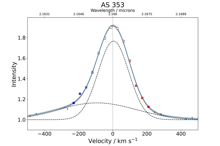
GRAVITY Collaboration: The GRAVITY young stellar object survey. IX.
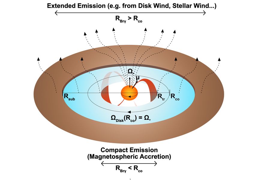
Fig. 1. Schematic depiction of the innermost parts of the circumstellar disk of a T Tauri star. Brγ emission in T Tauri stars is associated with the
concept of magnetospheric accretion, but outflows caused by certain types of disk or stellar winds (dashed lines) can heat the hydrogen gas to
the necessary temperatures to produce Brγ emission as well. Different origin mechanisms can be tied to different spatial scales. Magnetospheric
accretion flows (depicted in red) can only stably form in a compact region within the co-rotation radius Rco , where the gaseous disk rotates at the
same angular velocity Ω as the star. Spatially extended Brγ emission from outside Rco cannot be attributed to magnetospheric accretion and must
be caused by some other emission component. This figure specifically shows the common case of a non-axisymmetric magnetosphere, featuring a
tilt between the stellar rotational axis Ω∗ and the magnetic dipole µ. The obliquity of the magnetosphere leads to the formation of two accretion
columns, which funnel gas from a wide arc at the truncation radius onto one primary hot spot per hemisphere, as first suggested in Bertout et al.
(1988) and Calvet & Hartmann (1992). The equations and physical quantities relevant for the determination of the co-rotation radius Rco and the
magnetic truncation radius Rtr are discussed in Sect. 5. For the equations used to estimate the sublimation radius Rsub , which indicates the area at
which the disk becomes sufficiently hot to destroy dust grains, we refer to GRAVITY Collaboration (2021b).
results. Comparisons with synthetic data obtained from the mod- K-band beam combiner based at the ESO facilities of the VLTI
els can be found in Sect. 6, along with a wider discussion on at Cerro Paranal, Chile. The analysis of the Brγ emission region
magnetospheric accretion and the origin of Brγ in T Tauri stars relies exclusively on observations taken with the four Unit Tele-
scopes (UTs) with their 8.2 m primary mirrors. The Auxiliary
2. Scientific sample and observations Telescopes (ATs), while providing better coverage in the uv plane
and potentially higher spatial resolution at the longest baselines,
2.1. Sample are usually not sensitive enough to detect the relatively faint
emission signal of Brγ originating from T Tauri type stars. The
We have studied a total of seven T Tauri sources, which in standard UT configuration combines the four telescopes to a total
the context of this work will be referred to as the GRAVITY of six baselines, spanning up to 130 m in length on the ground
T Tauri sample. The targets in the sample consist of a number of λ
and providing a spatial resolution of up to 2B , which translates
mostly strong accretors with mass-accretion rates of the order of into 1.6–1.7 mas when observing in the near infrared between 2
10−8 M⊙ yr−1 , masses of less than 1.5 M⊙ , and stellar luminosi- and 2.4 micrometres. With the exception of S CrA N, all of the
ties ranging up to 4 L⊙ . The majority are mid K-type stars with sources were observed in single field mode, meaning the fringe
surface temperatures in the span between 4000 and 4900 K and data were simultaneously recorded on the separate detectors of
ages of 1–2 million yr or younger. Their individual properties are the instrument’s fringe tracker (FT) and science channel (SC).
summarised in Table 1. The FT data were recorded at low spectral resolution (R = 22)
in six spectral channels over the range of the entire K-band.
2.2. Observations
While the fringe tracker data in its own right can be utilised in the
The individual sources of the sample were observed between analysis of the K-band continuum, its main purpose with respect
2016 and 2021 with VLTI GRAVITY, the latest generation to the investigation of the hydrogen emission lines is to allow for
A59, page 3 of 40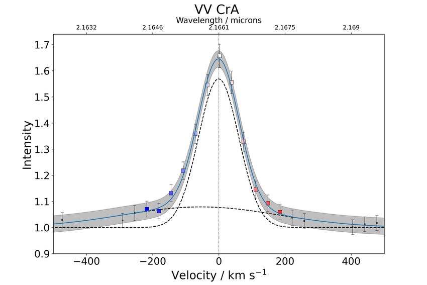
A&A 669, A59 (2023)

Table 1. Properties of the stars of the T Tauri sample.

   Name             Sp. type   T eff        d           M∗             L∗             R∗             Ṁacc         Age            References
                               [K]         [pc]        [M⊙ ]          [L⊙ ]          [R⊙ ]      [10−8 M⊙ yr−1 ]   [Ma]
   AS 353             K5       4450    399.6 ± 4.2    1 ± 0.2      3.9 ± 0.67     3.32 ± 0.29       7.9–45        ≤1            Rei et al. (2018),
                                                                                                                               Prato et al. (2003)
   RU Lup             K7       4050    157.5 ± 1.3    0.6 ± 0.2   1.64 ± 0.22     2.60 ± 0.17       1.8–30        1–2    Herczeg & Hillenbrand (2008),
                                                                                                                              Siwak et al. (2016)
   VV CrA SW          K7       4050    156.6 ±1.2     0.6 ± 0.2   1.73 ± 0.24     2.67 ± 0.19      3.33–22        1–2        Sullivan et al. (2019)

   TW Hya             K6       4200    60.14 ± 0.07   0.9 ± 0.1   0.41 ± 0.05     1.21 ± 0.07     0.13–0.23       4-12       Donati et al. (2011),
                                                                                                                              Venuti et al. (2019)
   S CrA N          K5-K6      4300    160.5 ± 2.2    0.9 ± 0.2   3.82 ± 0.54     3.52 ± 0.25       7.8–50        ≤1        Sullivan et al. (2019),
                                                                                                                              Gahm et al. (2018)
   DG Tau             K6       4200    125.2 ± 2.3    0.8 ± 0.2   1.58 ± 0.37     2.37 ± 0.28       4.6–74        1–2       White & Ghez (2001),
                                                                                                                          White & Hillenbrand (2004)
   DoAr 44          K2-K3      4840    146.3 ± 0.6    1.5 ± 0.2    1.61 ± 0.21    1.80 ± 0.12      0.63–0.9       3–6           Manara (2014),
                                                                                                                            Espaillat et al. (2010)

Notes. References are referring to the lower and upper limit Ṁacc literature values. We note that R∗ was computed from effective temperature and
stellar luminosity. Other properties were adopted from GRAVITY Collaboration (2021b).

longer integration times in the SC than would otherwise be fea-                       In the context of this work we focus on the analysis of the SC
sible by stabilising the fringes against small perturbations of the              data to extract information about the Brγ gas emission region,
atmosphere (Lacour et al. 2019). We made use of the FT capa-                     whereas FT data is only used in a supplemental manner as
bility to take the SC observations in GRAVITY’s high resolution                  described further below. For an overview of the treatment of the
mode (R = 4000) with a width of ∼5 Å, or 75 km s−1 , per chan-                   K-band continuum, based on the same data sets obtained with
nel, enabling us to spectrally resolve the Brγ feature and trace                 GRAVITY, we refer to the work of GRAVITY Collaboration
the gas kinematics over a range of up to ± six channels from the                 (2021b).
centre of the line, depending on the strength of the feature in the                   Each of the individual files obtained for all of our targets con-
individual sources.                                                              tains four sets of flux data coming from the four Unit Telescopes,
     The observations of the different targets are subdivided into a             six sets of normalised visibility amplitude data coming from the
set of short term runs of about 5 min in length, each of which was               six UT baselines, six corresponding sets of visibility phase data,
saved as a separate file, stretching over a total observation time               and four sets of closure phase data from the four unique closed
of around 1 1/2 hr for most of the objects, although the observa-                baseline triangles that can be formed by the UTs.
tion of DoAr 44 went on for notably longer with a total time of                       The individual files were merged before further analysis
slightly over 4 hours. Measurements of suitable calibrator stars                 using the post-processing routine of the GRAVITY pipeline,
in a sufficiently close part of the sky were predominantly taken                 effectively time-averaging our observables with a weighted mean
either up to 45 min before the beginning or after the end of the                 over the 1 1/2 h of observation. The data were globally shifted to
telescope run and thus potentially probing the sky under close                   the local standard of rest (LSR) to eliminate observational effects
but not entirely identical atmospheric conditions. For the 2021                  due to the earth’s rotation around the sun and the radial velocity
epoch of the RU Lup observation, no calibrator close to the tar-                 of the source.
get was available for the night, so that an object in a significantly                 The flux data were treated by first merging the four individual
different part of the sky had to be used for data calibration.                   telescope spectra and then normalising the Brγ peak to the sur-
     Weather conditions for the relevant nights were mostly sta-                 rounding continuum via a polynomial fit in the region between
ble with typical seeing values of around 0.5–0.7 arcseconds,                     2.1 and 2.2 µm. The normalised mean spectrum was further fit-
however, due to the relatively long observation of DoAr 44,                      ted with a Gaussian function in a region (2.15 and 2.18 µm)
we note a larger fluctuation of the seeing throughout the night                  closer to the Brγ peak to smooth out local fluctuations when
and deteriorating atmospheric conditions towards the end of the                  determining the line-to-continuum ratio on a channel to channel
run.                                                                             basis. For those objects in the sample which exhibit asymmetric
     The GRAVITY data on TW Hya, S CrA and DoAr 44 was                           line shapes, a combination of two single Gaussians was used to
previously published in GRAVITY Collaboration (2017b, 2020),                     fit the spectrum. We then consider the function value for a given
and Bouvier et al. (2020), respectively. A log of the observations               wavelength as the true line to continuum flux ratio for that wave-
of the T Tauri sample is given in Table 2.                                       length and use this value in our computations concerning the
                                                                                 size and photocentre shift as detailed in Appendix A. In order
                                                                                 to ensure the interpretation of the data remains meaningful, we
3. Data reduction and spectral calibration                                       implemented a selection criterion based on the strength of the
3.1. Pipeline reduction and post-processing                                      flux ratio in each channel relative to the continuum dispersion so
                                                                                 that only those channels that lie above a 2σ threshold are taken
The data were reduced and calibrated through the use of the stan-                into account for further analysis.
dard GRAVITY pipeline software provided by ESO (Lapeyrere                             For the visibility amplitudes, which we take as the root of
et al. 2014). A full account of the calibrated SC data from the                  the V 2 , we used FT data to normalise the science channel con-
observations is given in Appendix D.                                             tinuum around the Brγ line to the continuum value measured by

A59, page 4 of 40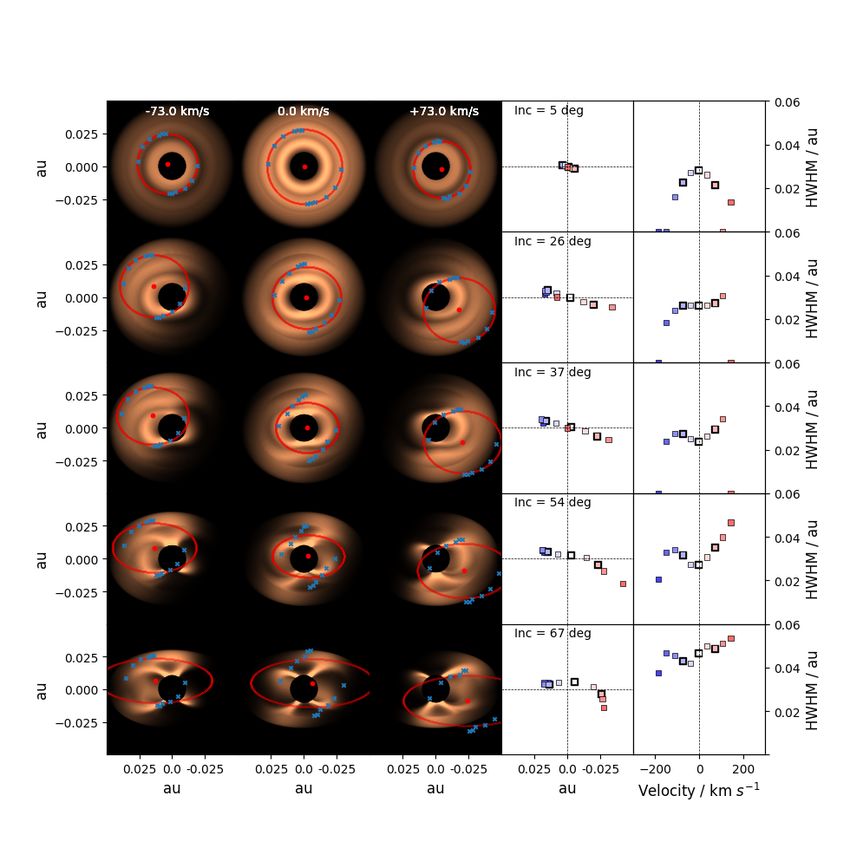
GRAVITY Collaboration: The GRAVITY young stellar object survey. IX.

Table 2. Log of observations.

         Source                 Date         Time (UTC)        Configuration      Calibrator      Airmass     Seeing [arcsec]     Files
         DG Tau             21.01.2019       01:31–03:06      U1-U2-U3-U4         HD 37491          1.59            0.65           10
         TW Hya             21.01.2019       06:59–08:24      U1-U2-U3-U4         HD 95470          1.03            0.51           13
         AS 353             21.04.2019       08:44–10:22      U1-U2-U3-U4         HD 183442         1.31            0.34           12
         RU Lup 2018        27.04.2018       03:23–04:30      U1-U2-U3-U4         HD 142448         1.27            0.57            8
         RU Lup 2021        30.05.2021       01:58–03:19      U1-U2-U3-U4         HD 99264          1.31            0.64            8
         S CrA N            20.07.2016       05:30–06:13      U1-U2-U3-U4         HD 188787         1.10            0.56            6
         VV CrA             20.06.2019       02:53–04:04      U1-U2-U3-U4         HD 162926         1.31            0.77            3
         DoAr 44            22.06.2019       02:04–05:46      U1-U2-U3-U4         HD 149562,        1.04            0.68           28
                                                                                  HD 147701,
                                                                                  HD 147578

Notes. Time denotes the beginning of the first and the last file of the observation.

the fringe tracker for the corresponding baseline. To this end, we           baselines shifted to the left or right, thus affecting the results
took an average continuum value from the FT channels, discard-               of the channel-by-channel analysis of those observables. The
ing the channel at the lowest wavelength as it is affected more              line feature in the differential phases is equally affected, as
strongly by atmospheric conditions and the meteorology laser                 S-shape signatures can be effectively suppressed and appear
operating at 1.908 µm. To determine the visibility value in each             single peaked.
of the considered spectral channels, a single peaked Gaussian                     We adjust for this effect by introducing a correction based on
function was then fitted to the data, similar to the treatment of the        a fit of the 24 individual spectra of each observational run to the
flux. The visibility phase data received an analogous treatment              known telluric lines close to Brγ. If the telluric lines are too weak
after a polynomial function was first fitted to and then subtracted          or the data too noisy to produce a proper fit, a master correction
from the data in order to obtain the differential phase between              based on an average shift is applied. An example of this, showing
line and continuum channels.                                                 the individual spectra before and after the correction, is shown
     We attempted to correct for the telluric effects from atmo-             in Fig. 2.
spheric absorption lines by using the calibrator spectra, but found               We found the overall effect of the correction to be more
that many of the calibrators were not suitable for this method               pronounced in the photocentre shift profiles derived from the
due to large photospheric absorption features broad enough to                differential phases, whereas the visibility data appeared to be
cover the telluric features. An alternative attempt, using an atmo-          relatively less affected. The general impact is highest on the
spheric model spectrum, to remove the telluric lines proved also             pure line quantities (see Appendix A), which is shown in Fig. 3.
to be problematic. Instead, we decided against a full correction             While the marginally changed shape of spectra and visibility sig-
and opted to restrain our analysis to a range of channels that falls         nals after the correction also affect the pure line observables, the
inside the two telluric features at 2.163446 and 2.168645 µm. We             dominant effect here stems from the relative shift between the
proceeded to remove the channels affected by those two features              mean spectrum and the interferometric observables. When com-
from the spectrum before attempting to fit the Gaussian pro-                 puting VLine from Eq. (A.1), a different combination of FL/C and
file as described above. Whilst we recognise that the flux ratios            Vtot values in each channel is used after the correction, as now the
obtained close to the telluric features obtained in this manner are          visibility peaks are better aligned with the mean spectral peak.
potentially incorrect, we propose that the overall impact of this            The difference is immediately obvious when comparing the pure
discrepancy on our results is negligible as low signal strengths             line visibilities in Fig. 3 between top and bottom. Before the cor-
in those areas means we do not consider those channels in our                rection, the peak of the visibility was shifted to the right with
analysis for the majority of our targets.                                    respect to the four-telescope mean spectral peak, resulting in
                                                                             comparatively large values for Vtot at much weaker flux ratios
                                                                             in the blue wing. Consequently, the pure line visibilities are
3.2. High-precision spectral calibration
                                                                             increasing as we move to higher wavelengths. After the correc-
A more detailed analysis of the flux recorded by the 4 UTs has               tion, the decreasing values for FL/C in the blue wing are paired
shown a systematic spectral shift of the spectra with respect to             with decreasing values in in the visibilities, leading to a peak in
known telluric absorption lines in the K-band. This shift, which             pure line visibilities that is roughly aligned with the peak in total
is on average of the order of 5 Å, is not affecting the individ-             visibilities.
ual UT spectra equally, leading to a misalignment between the                     The telluric shift has been detected in all of the data sets
4 Brγ lines recorded with the UTs. Such a misalignment not only              except for the 2021 epoch of RU Lup. The effect is currently
affects the flux values in the merged spectrum, but also the com-            understood to be connected to the old grism of the science spec-
putation of the complex visibilities by the pipeline during the              trometer and was consequently resolved with the grism upgrade
reduction process. This leads to a distortion of the Brγ line sig-           in October 2019, meaning all GRAVITY data taken after this
nature in both the visibility amplitudes and differential phases             month should no longer be affected.
for the different baselines, depending on the UTs involved. As
a practical consequence of this effect we noticed that the spec-             4. Data and methodology overview
trally resolved line features in the visibility amplitudes, which
are generally expected to be single peaked, were not well aligned            Through our GRAVITY observation, we obtained K-band spec-
with the peak of the mean spectrum and instead were for some                 tra between 2 and 2.4 microns, showing clear Brγ features at
                                                                                                                                A59, page 5 of 40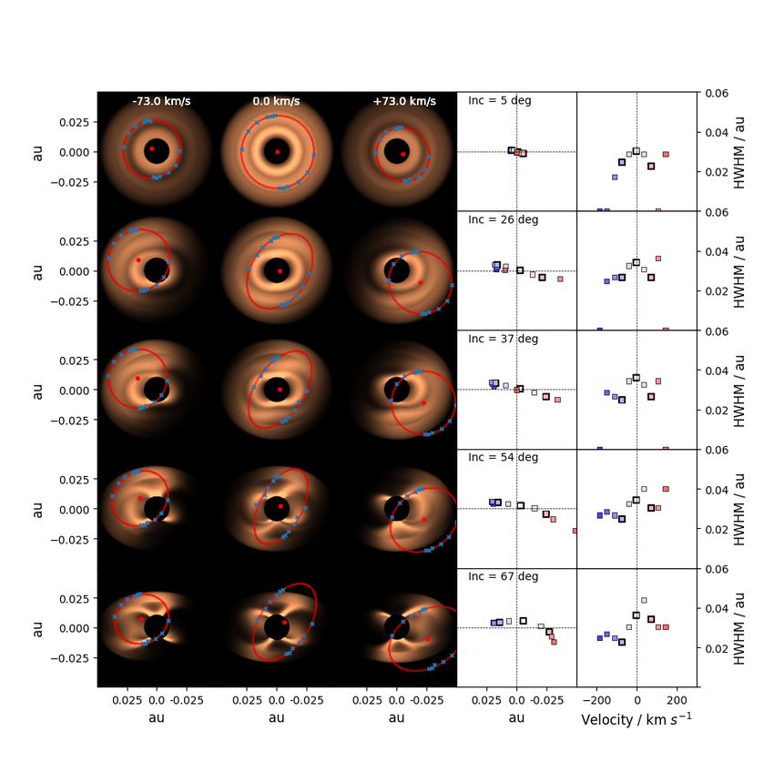
A&A 669, A59 (2023)

Fig. 2. Brγ spectra of the AS 353 observation, taken with the four unit
telescopes of the VLTI. Top: the spectra before the application of the       Fig. 3. Total and pure line visibilities for an exemplary baseline from
spectral calibration. The vertical line indicates the mean position of the   the AS 353 observation. Top: visibilities before the spectral correction
line peak. Before the correction, the individual spectra for most of our     was applied. Blue and grey shaded regions indicate the uncertainties on
objects were misaligned both with respect to the telluric lines and also     the total and pure line visibilities, respectively. Bottom: same baseline
between each other. Bottom: same spectra after they were brought into        after the correction. Especially with respect to the computation of the
alignment through the spectral calibration. The corrected spectra and        pure line visibilities, the change appears significant in the red wing of
recomputed observables were then further shifted to bring them to the        the signal.
local standard of rest (LSR).

                                                                             and surrounding continuum can be as high as 0.12 (Fig. D.3),
around 2.16 microns with peak line-to-continuum flux ratios                  compared to the relatively faint signals detected at the position
spanning a range of values from 1.91 in the extreme case of                  of Brγ for DoAr 44 with a line to continuum difference in
AS 353 down to only 1.19 for the faintest line we observed for               visibility of only about 0.01 at even the longest baselines.
DoAr 44. The uncertainties on the flux ratios, derived from the                  Noise levels can equally vary greatly, with low continuum
instrumental error bars given by the pipeline, are of the order of           dispersion in wavelength regions adjacent to the Brγ line again
0.01 for the majority of the T Tauri sample, although in the case            for RU Lup, where we measure a continuum standard deviation
of VV CrA we note a severe increase to around 0.03, even though              of 0.0023, compared to the very noisy data obtained for VV CrA
the dispersion of the continuum flux values remains comparable               (Fig. D.6) where the continuum standard deviation can go up to
to the dispersion found for the other sources.                               0.035.
    The continuum visibility data in the vicinity of the Brγ fea-                We found non-zero differential phases at the position of Brγ
ture for the different objects in the sample ranges from visibilities        at several baselines for each target in the sample, with typical
of about 0.7 to amplitudes close to 1, indicating that the total line        absolute phase values of around 0.5◦ –1◦ , although the largest
emission region and the surrounding continuum were partially                 measured differential phase goes up to 6.3◦ . S-shaped features,
resolved over the entire K-band at baseline lengths between 40               as expected for systems in rotation, can be observed for some
and 130 m for all of the targets. The Brγ visibilities signals are           sources at some baselines (e.g. RU Lup 2021, UT4-UT1, see
single peaked and in most cases well aligned with the position               Fig. D.3), but are rather exceptional and notably absent from
of the feature in the corresponding spectrum, see, for instance,             many other targets. The features appear single peaked in many
Fig. D.2.                                                                    cases, but the peak is not aligned with the line centre, suggesting
    There are clear distinctions in terms of visibility sig-                 that in such cases a potential S-shape might be masked by one of
nal strength at the Brγ line between the different sources.                  the two constituent peaks being somehow attenuated.
Particularly clear and strong features were observed in both                     The differential phase data is significantly more noisy
epochs of RU Lup, where the difference between Brγ peak                      when compared to the visibilities. Standard deviations in the

A59, page 6 of 40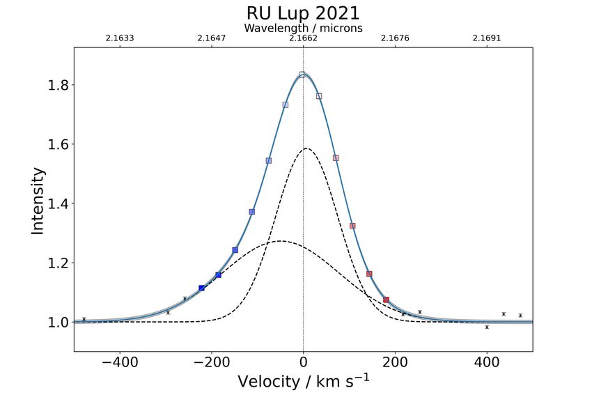
GRAVITY Collaboration: The GRAVITY young stellar object survey. IX.

Table 3. Results for equivalent widths, mass-accretion rates, and characteristic sizes of the Brγ emission region.

                                   AS353        RU Lup 2018     RU Lup 2021       TW Hya         DG Tau         DoAr 44          S CrA            VV CrA
   FL/C                             1.91            1.86            1.83            1.61           1.29           1.19            1.53              1.65
   FWHM [km s−1 ]                   233              183            187             121            224            137             175               150
   W10% [km s−1 ]                   594              607            420             241            445            274             524               416
   µHV [km s−1 ]                    −97             −55             −50            −183             –              –              −273             −75.49
   µLV [km s−1 ]                     3                2              6               1              –              –               3                0.84
                       −1
   FWHMHV [km s ]                   520              586            295             482             –              –              549              598.54
   FWHMLV [km s−1 ]                 204              154            154             116             –              –              170              141.32
   EW [Å]                       −19.62 ± 0.91 −16.82 ± 1.76     −13.47 ± 0.43   −7.11 ± 0.76   −5.80 ± 0.35   −2.65 ± 0.38    −8.71 ± 0.66      −10.09 ± 0.99
   Lacc [L⊙ ]                    3.07 ± 0.17   0.98 ± 0.12       0.76 ± 0.03    0.03 ± 0.00    0.33 ± 0.02     0.07 ± 0.01     1.74 ± 0.15       1.64 ± 0.19
   log Ṁacc,inst [M⊙ yr−1 ]    −6.38 ± 0.44    −6.76 ± 0.48    −6.87 ± 0.48    −8.74 ± 0.49   −7.40 ± 0.47   −8.46 ± 0.49    −6.56 ± 0.44      −6.52 ± 0.47
   Ṁacc,inst [10−8 M⊙ yr−1 ]    41.48+41.35
                                      −20.16
                                                 17.31+20.78
                                                      −8.54
                                                                 13.38+15.79
                                                                      −6.66
                                                                                  0.18+0.32
                                                                                      −0.1      3.95+4.44
                                                                                                    −2          0.35+0.38
                                                                                                                    −0.19      27.72+28.96
                                                                                                                                    −13.57
                                                                                                                                                 29.77+34.39
                                                                                                                                                      −14.59

   PA [◦ ]                         173 ± 3         99 ± 31        101 ± 31        130 ± 32      143 ± 12        137 ± 4          1±6               91 ± 6
   i[◦ ]                            41 ± 2          16+6
                                                      −8            20+6
                                                                      −8           14+6
                                                                                     −14          49 ± 4          32 ± 4          27 ± 3            32 ± 3
   Continuum HWHM [au]           0.28 ± 0.05     0.21 ± 0.06     0.21 ± 0.06    0.042 ± 0.003  0.13 ± 0.01     0.16 ± 0.02     0.17 ± 0.02       0.16 ± 0.01
   Brγ HWHM [au]                0.206 ± 0.003   0.076 ± 0.001   0.061 ± 0.001   0.029 ± 0.001 0.143 ± 0.004   0.050 ± 0.002   0.071 ± 0.011     0.081 ± 0.005
   Rtr [au]                      0.04 – 0.08     0.04 – 0.07     0.04 – 0.08     0.05 – 0.07   0.05 – 0.09      0.09 – 0.11    0.05 – 0.10       0.04 – 0.07
   Rco [au]                          0.10           0.04            0.04            0.05           0.06            0.05            0.04              0.10
   Continuum HWHM [R∗ ]         18.13 ± 3.59     17.36 ± 5.10   17.36 ± 5.10    7.47 ± 0.70    11.32 ± 1.61   19.07 ± 2.69    10.38 ± 1.42      12.64 ± 1.04
   Brγ HWHM [R∗ ]               13.32 ± 1.16     6.32 ± 0.43    5.01 ± 0.35     5.13 ± 0.33    12.93 ± 1.56    5.93 ± 0.47     4.36 ± 0.75      6.56 ± 0.59
   Rtr [R∗ ]                     2.83 – 5.30      3.28 – 6.14    3.53 – 6.61    8.31 – 12.35    4.50 – 8.42   10.62 – 12.68    3.36 – 6.29       2.86 – 5.36
   Rco [R∗ ]                        6.47             3.31           3.31            8.89           5.44           5.96            2.44              7.25

Notes. FL/C is the total line to continuum flux ratio at the centre of the line. FWHM and W10% are the line widths at 50 and 10% of the peak
flux, respectively. µ is the position of the high (HV) or low velocity (LV) component from the double Gaussian fit to the spectrum. The Brγ half-
flux radius (HWHM) is given for the central channel. Rco , continuum HWHM, PA, and i were adopted from GRAVITY Collaboration (2021b).
Accretion luminosities were estimated from the line luminosities based on the empirical relationship in Eq. (1). The instantaneous mass-accretion
rates were then computed as in Eq (2). Rtr is given based on Eq. (4) for magnetic field strengths between 1 and 3 kG and using the mass-accretion
rates derived from the equivalent widths (EW). The asymmetric error bars on the absolute values of Ṁacc,inst represent the 25th and 75th percentiles
of the distribution. Other error bars denote 1σ uncertainties.

continuum adjacent to Brγ, even for sources with clear differ-                    derived properties across the different velocity components of
ential phase Brγ peaks, are on average the order of 0.4◦ . For the                the Brγ line, see, for example, Fig. 6. A full explanation of the
very noisy data of VV CrA the continuum dispersion even goes                      process is given in Appendix A.
up to 2◦ in standard deviation.
    The closure phases at the position of Brγ are consistent with
the closure phases of the nearby continuum throughout the sam-                    5. Results
ple with no clear Brγ signal visible for any of the sources. The                  5.1. General results
continuum closure phases for most of our objects are close to 0◦ ,
although small offsets of around 1◦ can be detected at certain                    In this section we first present a breakdown of the general results
baseline triangles for AS 353, RU Lup, and DoAr 44 (Figs. D.1,                    obtained from the GRAVITY T Tauri data, introduce some
D.3, and D.7, respectively). For VV CrA (Fig. D.6) we found                       additional concepts relevant to the interpretation, and give an
again a comparatively large dispersion of closure phase values,                   overview over the global trends we were able to identify across
with standard deviations across the different triangles reaching                  the entire sample. In the following sections, we then proceed
up to 4◦ .                                                                        to go over each source individually in detail and contextualise
    The data were treated by using the total line to continuum                    our findings by drawing upon relevant references, if and where
flux ratio and continuum quantities to remove the influence of the                available. Table 3 summarises key results concerning the char-
continuum on the interferometric observables. This way a ‘pure                    acteristics of the Brγ emission region and accretion properties,
line’ Brγ visibility and differential phase was extracted from the                respectively. Figures 4 and 5 serve as a visual overview of the
total observables in each of the chosen spectral channels and                     sample results with regards to the most important criteria we use
then further used to determine the size and photocentre of the                    to interpret our results.
Brγ emission region. Based on a simple geometric Gaussian disk                         The sample consists of mostly strong Brγ emitters, with nor-
model (Berger & Segransan 2007), we extracted the half-flux                       malised peak line to continuum flux ratios between 1.91 and 1.53
radius (or half width half maximum, HWHM) in each channel,                        for six out of our eight data sets and ranging down to 1.19 for
as well as the relative offset of the photocentre with respect to                 the weakest emitter DoAr 44. Many of the objects exhibit line
the position of the continuum photocentre. This treatment was                     shapes that are asymmetric, featuring an excess of blueshifted
applied to a number of spectral channels based on the previously                  emission. We approximate this asymmetry by fitting a superpo-
explained flux selection criterion to analyse the change of those                 sition of two Gaussian functions to the data, basically dividing

                                                                                                                                              A59, page 7 of 40
A&A 669, A59 (2023)

                                                                             line luminosities for each object from the equivalent widths and
                                                                             K-band magnitudes from 2MASS (Cutri et al. 2003). We then
                                                                             used the empirical relationship from Alcalá et al. (2014),
                                                                                        !                 !
                                                                                   Lacc             LLine
                                                                             log          = a · log         +b                               (1)
                                                                                   L⊙                L⊙

                                                                             with a = 1.16 ± 0.07 and b = 3.6 ± 0.38, to estimate the accretion
                                                                             luminosities and subsequently determined the corresponding
                                                                             mass-accretion rates via (Hartmann et al. 1998)

                                                                                                 !−1
                                                                                           R∗                  R∗             R∗
                                                                             Ṁacc = 1 −               Lacc       ≈ 1.25Lacc     ,           (2)
                                                                                           Rin                GM∗            GM∗

                                                                             which describes the relationship between the gravitational
                                                                             energy released and radiated away by the mass falling in from
                                                                             the truncation radius. For the right hand side approximation we
                                                                             follow the common convention of using Rin ≈ 5 R∗ as a typical
                                                                             size for truncation radii.
                                                                                  These results are summarised in Table 3. They are also
                                                                             shown in Fig. 4, where we present both the instantaneous mass-
                                                                             accretion rates as well as a range based on the lowest and highest
                                                                             previous estimates found in the literature. Based on this compar-
                                                                             ison, we found that our mass-accretion rates tend to fall into the
                                                                             range established by past observations, even if mostly towards
                                                                             the higher end for the stronger accretors. The uncertainties on the
                                                                             coefficients a and b of Eq. (1) translate into relatively large and
                                                                             asymmetric error bars on the absolute value of Lacc and conse-
                                                                             quently also Ṁacc . We used a Monte-Carlo approach to determine
                                                                             the final uncertainties on the accretion rate, rather than Gaussian
                                                                             error propagation not applicable here.
                                                                                  We fitted the visibility data with a 2D Gaussian in order
                                                                             to find the half-flux radii (HWHM) of the pure Brγ emis-
                                                                             sion region, using the inclination and position angles of the
Fig. 4. Relationships between Brγ emission region sizes and selected         K-band continuum emission region presented in GRAVITY
stellar properties. Top: fitted HWHM of the Brγ pure line emission           Collaboration (2021b) to constrain those two parameters in our
region of the central channel versus the mass-accretion rate. The lat-       fit. The HWHMs we obtained through this process are, across
ter is depicted in two forms: once as a grey bar which denotes the range     the entire sample, of the order of less than 0.21 au at their great-
of Ṁ values found in the literature on the respective source, then as the
                                                                             est extent, ranging down to regions as compact as 0.03 au. In
instantaneous mass-accretion rate, which was derived from the equiva-
lent width of the GRAVITY Brγ spectra. The colour coding represents          terms of stellar radii, the central channel sizes vary from up
the classification of the sample objects as either weak (green) or inter-    to 13 R∗ to less than 5 R∗ , although the majority of objects
mediate to strong accretors (red). Most of the T Tauri stars cluster in      show clustering (see Figs. 4 and 5) in a range from 4 to 7 R∗ ,
a 4–7 R∗ range, which is of the order of typical magnetospheric sizes.       which is fairly typical for magnetospheric radii (Bouvier et al.
Bottom: Brγ HWHM versus accretion luminosities. The colour coding            2007). This clustering can be observed across the entire range of
corresponds to the upper plot.                                               mass-accretion rates of our small sample, so that a correlation
                                                                             between those sizes and accretion rates cannot be established
                                                                             here. Equally, within our sample we do not detect a clear cor-
the feature into a narrow centred low velocity component and                 relation of those Brγ sizes with the luminosity of the objects, as
a broader offset high velocity component. Whether these Gaus-                opposed to the NIR continuum sizes, which were shown to corre-
sian components can necessarily be directly attributed to specific           late as per R ∝ L1/2 (GRAVITY Collaboration 2021b). However,
physical phenomena, such as additional outflows on top of an                 it is apparent from Fig. 5 that the two weakest accretors in the
accreting magnetosphere, is not certain. Inverse P Cygni fea-                sample (TW Hya and DoAr 44) also show most clearly an emis-
tures, as expected to be seen when observing magnetospheric                  sion region smaller than the co-rotation radius, whereas most of
accretion columns at low inclination, are generally absent from              the other objects show Brγ emission coming from beyond the
the line profiles of the sample, even for those objects observed             co-rotation radius.
at a close to pole-on configuration, such as TW Hya. The width                    Changes in HWHM in the spectral channel across the Brγ
and offset of the broad component, and thus of the total emission            line can be significant, with largest to smallest size-in-channel
line, can vary significantly throughout the sample, even between             ratios being around 1.2–1.5 for many of the objects, although in
two epochs of the same target (RU Lup), although the overall                 extreme cases this can go up to almost 2, whilst others show a
strength of the asymmetry correlates with the peak flux ratio                relatively flat profile relative to their error bars. Under a magne-
and is also reflected in the equivalent widths. We computed the              tospheric accretion scenario, a decrease of size towards the edges

A59, page 8 of 40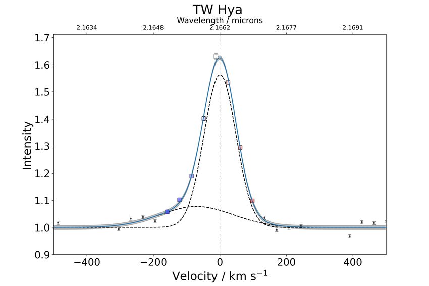
GRAVITY Collaboration: The GRAVITY young stellar object survey. IX.

Fig. 5. Sample overview for emission region sizes and photocenter shifts. Top: Brγ half-flux radii (yellow), compared to K-band NIR continuum
half-flux radii (red) and co-rotation radii (green) across the sample. We note that Brγ region and continuum HWHMs are based on a Gaussian
disk and a Gaussian ring model, respectively, which should approximately reflect the differences in the morphology of both regions. The objects
are given in order of descending mass-accretion rate. Bottom: the distribution of photocentre shift angles across the line for the entire sample. The
x-axis shows the minimum difference angle between the relative shift vector and the position angle of the continuum disk. The white channel serves
as the point of reference for the relative shift vector. An angle of 0◦ means the photocentre shift vector is aligned with the disk axis, as would for
example be expected for a disk in rotation. A difference angle of 90◦ indicates that the shift vector is perpendicular to the disk axis. A clustering
of points close to a certain difference angle indicates an alignment of the photocentre shifts along a preferential axis. VV CrA shows a monoaxial
distribution of photocentres, while for other targets more complex profiles with multiple alignments are indicated. The number stated in brackets
after the object name gives the average error on the angle for the five central channels.

of the line (i.e. higher velocities) would be naively expected, as          an increase as we move to higher velocities. These mixed pro-
the gas at the highest velocities should be in free fall close to           files could be indicative of a multi-component Brγ emission
the star. In our sample, only one source (TW Hya) clearly shows             region, although in many cases the extent of these more complex
this decrease, whereas most of the other objects show either a              signatures is within the uncertainties.
straight increase with a minimum at the centre channel or even                   An important point of reference in the search for the origin
a mixed profile with a decreasing size at low velocities and then           of Brγ emission is the co-rotation radius, since we know that the

                                                                                                                                   A59, page 9 of 40
A&A 669, A59 (2023)
inner disk must be truncated inside the Rco so that stable mag- within or close to 1 R∗ , although such a compact concentration
netospheric accretion columns can form. If the dominant driver of photocentres does not necessarily correlate with the size of
of Brγ emission is magnetospheric accretion, we expect that the the emission region. The photocentre profiles are complex and
Brγ emission region would be of the order of the co-rotation not easily classified, although a broad distinction can be made
radius or even slightly more compact. The co-rotation radius is between targets that show quasi-rotational profiles, featuring dis-
defined as the radius at which the angular velocity of the rotating tinct blue and red arms aligned along a common axis, targets
disk matches the angular velocity of the star Ω∗ (Bouvier 2013): with compact profiles that lack any clear structures, and com-
plex profiles which again appear potentially as a superposition
!1/3
GM∗ of multiple components. In Fig. 5 we give an overview over
Rco = . (3) the possible alignment of the photocentre shifts across the line
Ω2∗
with different axes. To account for the offset of the profiles from
Stellar angular velocities are determined from measurements the plot centre, we compute the difference vectors between each
of the rotational period of the star or the v sin(i). We refer to point and the centre channel (shown as a white square) and then
GRAVITY Collaboration (2021b) for the relevant values for our compute the minimum angular difference between the angle of
sample objects. The co-rotation radii are given in Table 3. Of the difference vector and the NIR continuum disk axis position
course, the best way to determine whether the size of the Brγ angle. The resulting value is a measure of how well aligned the
emission region corresponds to the size of the magnetosphere photocentre offsets are relative to the disk axis. The plot can be
in any object would be to compare the region size against the interpreted in a meaningful way by considering the degree of
magnetospheric truncation radius directly. The truncation radius clustering, and at which angles the clustering occurs. A concen-
can be computed from stellar parameters, if the strength of the tration of points in a narrow angular range (AS 353) indicates
magnetic dipole field is known: that the photocentre shift is aligned along a single axis. If the
clustering range is close to zero, the photocentres are aligned
with the disk semi-major axis, which is something that would
B34/7 R12/7
Rtr = 12.6 2
1/7 2/7
. (4) be expected from a disk in Keplerian rotation. If the points clus-
M0.5 Ṁ−8 ter at 90◦ , the photocentres might be aligned with some form of
polar outflow (red wing in DG Tau). An even spread of points
In this notation we follow the convention used in Hartmann et al. indicates an absence of recognisable structures and a random
(2016), for example. We note that M0.5 is the stellar mass in distribution of photocentres (TW Hya). The figure clearly shows
units of 0.5 M⊙ , R2 the stellar radius in units of 2 R⊙ , B3 the the previously introduced distinction between simple alignments
surface field strength of the dipolar magnetic field at the stel- and complex patterns, where we see multiple clusters (DG Tau
lar equator in kG, and Ṁ−8 the mass-accretion rate in units of and RU Lup).
10−8 M⊙ yr−1 . The resulting truncation radius is given in units It is important to remember that the differential phases track
of R⊙ . The derivation is conceptually discussed in Bessolaz et al. the relative offset of the Brγ emission region from the over-
(2008). all photocentre of the continuum. In Fig. 6, for example, the
Measurements of magnetic field strengths in T Tauri stars centre of the plot is the combined photocentre of the star and
are scarce, so that we cannot rely on the truncation radius as other continuum emitting components such as the dusty disk.
a primary criterion to identify strong magnetospheric accretion If the dusty disk is perfectly centrosymmetric, its own photo-
cases. Even so, we can still use general estimates of Rtr as com- centre coincides with that of the star and the overall continuum
plementary information. Building upon the approach laid out in photocentre matches the position of the star. If the continuum
GRAVITY Collaboration (2021b), we set a range of 1–3 kG for photocentre, however, is not centrosymmetric, either offset from
B and compute the truncation radii for this range as presented in the star or with an asymmetric brightness distribution, then the
Table 3 from the relevant stellar properties. zero position in those plots can significantly deviate from the
An overview of the emission region sizes in the cen- stellar position. We therefore make use of the closure phases
tral line channels, compared to the respective co-rotation radii to extract information about the continuum asymmetry. For the
and the NIR K-band continuum sizes taken from GRAVITY majority of our sample objects the closure phases themselves are
Collaboration (2021b), can be found in Fig. 5. The sample close to zero and thus suggest a centrosymmetric continuum. We
can generally be divided into targets with emission regions then instead use the uncertainty given by the phase dispersion to
of the order of the co-rotation radius (DoAr 44, TW Hya), derive an uncertainty on the stellar position. To do this we fol-
those with more extended Brγ emission than the co-rotation low GRAVITY Collaboration (2021b) by fitting an azimuthally
radius, but still close to typical magnetospheric radii around modulated ring model to the continuum closure phase data. The
5 R∗ (RU Lup, S CrA N, and VV, CrA SW), and those with results are depicted as red circles on the photocentre profile
highly spatially extended Brγ regions outside the typical range plots, showing that indeed in the majority of the cases the centre
of magnetospheric sizes (AS 353, DG Tau). This separation channel photocentre could conceivably be centred on the stellar
partially corresponds to the distinction between weak accretors position.
( Ṁacc < 1 × 10⁻⁸ M⊙ yr−1 , again DoAr 44 and TW Hya) and the
intermediate to strong accretors, which we indicated in Fig. 4 via
the different colours. While the weak accretors do appear to con- 5.2. Individual results
form to the co-rotation criterion with compact emission regions, 5.2.1. AS 353
the situation is more complex for objects with higher accretion
rates, as there is no clear correlation between the relative region With a peak line to continuum flux ratio of 1.91 and an equivalent
sizes and the mass-accretion rates for those targets. width of −19.6 Å, AS 353 (Fig. 6) is the strongest Brγ emitter in
Magnitudes for the observed photocentre displacements are the GRAVITY T Tauri sample. These measurements are consis-
of the order of 0.07 au or below. For multiple targets the entire tent with the results of a spectroscopic survey of young binaries
photocentre profile across the line is sufficiently compact to be done in 1996 by Prato et al. (2003), who found an equivalent
A59, page 10 of 40GRAVITY Collaboration: The GRAVITY young stellar object survey. IX.
comparing these quantities, it is important to point out a cer-
tain amount of confusion surrounding the distance estimate to
the AS 353 system. Since the system is thought to be connected
with the Aquila star forming region (Rice et al. 2006) and thus to
the complex of dark interstellar clouds of the Aquila rift, accu-
rate measurements of the distance have historically been difficult
to obtain. Previous works such as Edwards & Snell (1982) refer
to a distance of 150 pc, which was also adopted by Prato et al.
(2003) with a estimated error of 50 pc based on the idea that
AS 353 is in front of the Aquila rift at 200 ± 100 pc (Dame &
Thaddeus 1985). More recent high accuracy parallax measure-
ments of AS 353 taken by Gaia and released as part of DR2
and DR3 put the binary at a comparatively remote 400 pc (Gaia
Collaboration 2020), which is the value we adopt in this paper.
This is supported by other recent studies covering parts of the
Aquila rift, such as the work of Ortiz-León et al. (2017), which
presents astrometric measurements that put the WS40/Serpens
cloud complex at 436 ± 9.2 pc. Still, even relatively recent pub-
lications like the interferometric study of Eisner et al. (2014) use
the 150 pc estimate to convert their angular scales into physi-
cal sizes. For the Brγ emission region size Eisner et al. (2014)
report an angular ring diameter of 1.06 mas and a subsequent
ring radius of 0.08 au, which, if converted to the more recent
distance measurements, would translate to a radius of 0.21 au.
This, within a 1σ error bar, agrees with our findings, despite the
fact that their model does not take into account the relatively high
inclination of 41◦ of the inner disk of AS 353. Conversely, if our
results were to be converted into a physical size based on a 150 pc
distance, we would obtain a half flux radius of 0.077 au, meaning
something more compact than the co-rotation radius. However,
based on the fact that the most recent distance measurements for
AS 353 independently came to similar results, we consider the
400 pc estimate to be robust. As such, the very large extent of
the emission region indicates that the Brγ emission is likely pro-
duced through some form of disk wind outflow launched from
the inner gaseous disk.
This could be supported by the spatial profile of the Brγ
line photocentres, which shows similarity to a rotational profile,
albeit not aligned with the disk and severely truncated in the blue
wing. It is possible that such an asymmetric structure, with a
maximum photocentre displacement of 0.039 au, or 2.5 R∗ , in the
red wing, is caused by the interplay of disk and jet. The AS 353
system is connected to the Herbig-Haro object HH32 and drives
a large-scale outflow at a very high inclination of 70◦ (Curiel
et al. 1997) with a fainter blue component and multiple more
prominent redshifted knots. At a smaller scale, Hα emission
originating from a blueshifted jet was reported at a position angle
of (111 ± 18)◦ by (Takami et al. 2003). This is, within the respec-
tive uncertainties, close to perpendicular to the NIR continuum
disk axis of (173 ± 3)◦ (GRAVITY Collaboration 2021b).
Assuming that the weaker emission in the blue knot observed
in HH32 translates to a similar asymmetry for the small-scale
jet, a superposition of two distinct photocentre shift profiles, one
Fig. 6. Spectrum (top), size (middle), and photocentre shift (bottom) aligned with the jet axis and the other coming from the rotating
profiles for AS 353. Shaded regions indicate uncertainties. base of a disk wind and thus aligned with the disk semi-major
axis, could lead to the observed distribution of photocentres.
This is also supported by the closure phase data, which indicates
width of −21.1 Å for the Brγ emission line of this object. We do that the position of the star is consistent with the centroid of the
not find a significant change in size across the Brγ line for the central velocity channel within an uncertainty of 0.026 au.
emission region, with all channels appearing consistent within
their respective uncertainties with a half flux radius of 0.206 au 5.2.2. RU Lup
at the centre of the line. This puts the emission region at about
twice the size of the co-rotation radius at 0.1 au, but still well RU Lup was observed in two distinct epochs in 2018 and 2021
within the NIR continuum HWHM of 0.28 au. However, when (Fig. 7). It appears as the second strongest Brγ emitter of our
A59, page 11 of 40You can also read