Algorithm Theoretical Baseline Document for Sentinel-5 Precursor: Carbon Monoxide Total Column Retrieval - European Space ...
←
→
Page content transcription
If your browser does not render page correctly, please read the page content below
Algorithm Theoretical Baseline
Document for Sentinel-5
Precursor:
Carbon Monoxide Total Column
Retrieval
Jochen Landgraf, Joost aan de Brugh, Remco A. Scheepmaker,
Tobias Borsdorff, Sander Houweling, Otto P. Hasekamp

 document number : SRON-S5P-LEV2-RP-002
 CI identification   : CI-7430-ATBD
 issue               : 2.2.0
 date                : 2021-02-16
 status              : released

S5P ATBD draft                                                 SRON-S5P-LEV2-RP-002
issue 2.2.0, 2021-02-16 – released                                       Page 2 of 82

Document approval record
                  digital signature

 prepared:

                    Michael Buchwitz and Thomas Krings
 checked:           Institute of Environmental Physics (IUP)
                    University Bremen, Germany

 approved PM:

 approved PI:
S5P ATBD draft                                                                     SRON-S5P-LEV2-RP-002
issue 2.2.0, 2021-02-16 – released                                                           Page 3 of 82

Document change record
 issue    date          item               comments
 0.0.1    2012-07-09    All                 lnitial draft version
 0.0.2    2012-11-23    Appendix A          Appendix added
 0.0.2    2012-11-23    Sec. 9              Hardware requirement updated
                                            Document revised according to
 0.5.0    2013-06-04    all
                                            SRR/PDR review Feb. 2013
                                            Document revised according to
 0.5.0    2013-06-21    all
                                            internal review June 2013
                                            Document revised according to
 0.9.0    2013-11-30    all
                                            external review September 2013
 0.9.1    2013-12-03    sec. 9              Section 9 ’Feasibility’ revised
 0.10.0   2014-04-15    app. B              SWIR pre-processor introduced
                        app. C              Appendix C ’HDO/H2 O’ revised
                                            Section added including tables
 0.11.0   2014-09-30    sec. 8
                                            on algorithm input and output
                        app. B              Appendix B revised
                                            Cloud filter analysis extended to
 0.11.1   2014-12-16    sec. 5.2.1
                                            one year GOSAT data
                                            Estimated computational effort now based
                                            on cloud filter performance for one year of
                        sec. 9.1
                                            GOSAT data (no significant change
                                            regarding computational cost)
                                            Update of algorithm input/output satisfying
 0.13.0   2015-09-08    sec. 8.3 and 8.4    project unit definition. Update for limited
                                            release to S5p Validation Team
 0.13.0   2015-12-09    all                 References updated, typos corrected
                                            Document revised according to
 1.00     2016-02-05    all
                                            internal review Dec. 2015
                                            appendix TROPOMI HDO/H2O retrievals removed
 1.10     2018-06-15    all
                                            section Examples of TROPOMI CO data added
                                            sections Validation and Examples of TROPOMI CO data removed
                                            section A posteriori destriping of the level-2 data added
 2.20     2021-02-16    all
                                            manuscript updated to reference
                                            the new cross sections used based on SEOM-IAS
S5P ATBD draft SRON-S5P-LEV2-RP-002 issue 2.2.0, 2021-02-16 – released Page 4 of 82 Contents Document approval record . . . . . . . . . . . . . . . . . . . . . . . . . . . . . . . . . . . . . . . . . . . . . . . . . . . . . . . . . . . . . . . . . . . . . . . . . . . . . . . . 2 Document change record . . . . . . . . . . . . . . . . . . . . . . . . . . . . . . . . . . . . . . . . . . . . . . . . . . . . . . . . . . . . . . . . . . . . . . . . . . . . . . . . . . 3 List of Tables . . . . . . . . . . . . . . . . . . . . . . . . . . . . . . . . . . . . . . . . . . . . . . . . . . . . . . . . . . . . . . . . . . . . . . . . . . . . . . . . . . . . . . . . . . . . . . . . 5 List of Figures . . . . . . . . . . . . . . . . . . . . . . . . . . . . . . . . . . . . . . . . . . . . . . . . . . . . . . . . . . . . . . . . . . . . . . . . . . . . . . . . . . . . . . . . . . . . . . . 6 1 Introduction . . . . . . . . . . . . . . . . . . . . . . . . . . . . . . . . . . . . . . . . . . . . . . . . . . . . . . . . . . . . . . . . . . . . . . . . . . . . . . . . . . . . . . 9 1.1 Identification . . . . . . . . . . . . . . . . . . . . . . . . . . . . . . . . . . . . . . . . . . . . . . . . . . . . . . . . . . . . . . . . . . . . . . . . . . . . . . . . . . . . . . . 9 1.2 Purpose and objectives . . . . . . . . . . . . . . . . . . . . . . . . . . . . . . . . . . . . . . . . . . . . . . . . . . . . . . . . . . . . . . . . . . . . . . . . . . . 9 1.3 Document overview . . . . . . . . . . . . . . . . . . . . . . . . . . . . . . . . . . . . . . . . . . . . . . . . . . . . . . . . . . . . . . . . . . . . . . . . . . . . . . . 9 2 Applicable and reference documents . . . . . . . . . . . . . . . . . . . . . . . . . . . . . . . . . . . . . . . . . . . . . . . . . . . . . . . . . 10 2.1 Applicable documents . . . . . . . . . . . . . . . . . . . . . . . . . . . . . . . . . . . . . . . . . . . . . . . . . . . . . . . . . . . . . . . . . . . . . . . . . . . . 10 2.2 Standard documents . . . . . . . . . . . . . . . . . . . . . . . . . . . . . . . . . . . . . . . . . . . . . . . . . . . . . . . . . . . . . . . . . . . . . . . . . . . . . . 10 2.3 Reference documents . . . . . . . . . . . . . . . . . . . . . . . . . . . . . . . . . . . . . . . . . . . . . . . . . . . . . . . . . . . . . . . . . . . . . . . . . . . . 10 2.4 Electronic references . . . . . . . . . . . . . . . . . . . . . . . . . . . . . . . . . . . . . . . . . . . . . . . . . . . . . . . . . . . . . . . . . . . . . . . . . . . . . 14 3 Terms, definitions and abbreviated terms . . . . . . . . . . . . . . . . . . . . . . . . . . . . . . . . . . . . . . . . . . . . . . . . . . . . 15 3.1 Acronyms and abbreviations . . . . . . . . . . . . . . . . . . . . . . . . . . . . . . . . . . . . . . . . . . . . . . . . . . . . . . . . . . . . . . . . . . . . . 16 4 Remote Sensing of Carbon Monoxide . . . . . . . . . . . . . . . . . . . . . . . . . . . . . . . . . . . . . . . . . . . . . . . . . . . . . . . . 18 4.1 Algorithm heritage. . . . . . . . . . . . . . . . . . . . . . . . . . . . . . . . . . . . . . . . . . . . . . . . . . . . . . . . . . . . . . . . . . . . . . . . . . . . . . . . . 18 4.2 Carbon Monoxide level-2 requirements . . . . . . . . . . . . . . . . . . . . . . . . . . . . . . . . . . . . . . . . . . . . . . . . . . . . . . . . . . 19 5 Algorithm Description. . . . . . . . . . . . . . . . . . . . . . . . . . . . . . . . . . . . . . . . . . . . . . . . . . . . . . . . . . . . . . . . . . . . . . . . . . . 21 5.1 Forward model . . . . . . . . . . . . . . . . . . . . . . . . . . . . . . . . . . . . . . . . . . . . . . . . . . . . . . . . . . . . . . . . . . . . . . . . . . . . . . . . . . . . 21 5.2 Inversion . . . . . . . . . . . . . . . . . . . . . . . . . . . . . . . . . . . . . . . . . . . . . . . . . . . . . . . . . . . . . . . . . . . . . . . . . . . . . . . . . . . . . . . . . . 28 5.2.1 Methane cloud filter . . . . . . . . . . . . . . . . . . . . . . . . . . . . . . . . . . . . . . . . . . . . . . . . . . . . . . . . . . . . . . . . . . . . . . . . . . . . . . . 28 5.2.2 Tikhonov regularisation for CO column retrieval . . . . . . . . . . . . . . . . . . . . . . . . . . . . . . . . . . . . . . . . . . . . . . . . 29 5.2.3 Tikhonov regularisation for stability . . . . . . . . . . . . . . . . . . . . . . . . . . . . . . . . . . . . . . . . . . . . . . . . . . . . . . . . . . . . . . 32 5.2.4 Step control . . . . . . . . . . . . . . . . . . . . . . . . . . . . . . . . . . . . . . . . . . . . . . . . . . . . . . . . . . . . . . . . . . . . . . . . . . . . . . . . . . . . . . . . 32 5.2.5 Unphysical values . . . . . . . . . . . . . . . . . . . . . . . . . . . . . . . . . . . . . . . . . . . . . . . . . . . . . . . . . . . . . . . . . . . . . . . . . . . . . . . . . 33 5.3 Numerical Implementation and Data Product . . . . . . . . . . . . . . . . . . . . . . . . . . . . . . . . . . . . . . . . . . . . . . . . . . . 33 5.4 Molecular optical properties . . . . . . . . . . . . . . . . . . . . . . . . . . . . . . . . . . . . . . . . . . . . . . . . . . . . . . . . . . . . . . . . . . . . . . 33 5.5 Micro-physical properties of the scattering layer . . . . . . . . . . . . . . . . . . . . . . . . . . . . . . . . . . . . . . . . . . . . . . . . 35 5.6 State vector, ancillary parameters and a priori knowledge . . . . . . . . . . . . . . . . . . . . . . . . . . . . . . . . . . . . . 35 5.7 Data product . . . . . . . . . . . . . . . . . . . . . . . . . . . . . . . . . . . . . . . . . . . . . . . . . . . . . . . . . . . . . . . . . . . . . . . . . . . . . . . . . . . . . . . 36 6 Common aspects with other algorithms. . . . . . . . . . . . . . . . . . . . . . . . . . . . . . . . . . . . . . . . . . . . . . . . . . . . . . 37 7 Error analysis . . . . . . . . . . . . . . . . . . . . . . . . . . . . . . . . . . . . . . . . . . . . . . . . . . . . . . . . . . . . . . . . . . . . . . . . . . . . . . . . . . . . 38 7.1 Performance analysis for generic scenarios . . . . . . . . . . . . . . . . . . . . . . . . . . . . . . . . . . . . . . . . . . . . . . . . . . . . . 38 7.2 Performance Analysis for generic scenarios . . . . . . . . . . . . . . . . . . . . . . . . . . . . . . . . . . . . . . . . . . . . . . . . . . . . 40 7.3 Geophysical test scenario for measurements over China . . . . . . . . . . . . . . . . . . . . . . . . . . . . . . . . . . . . . . 46 7.4 Robustness of the CO retrieval with respect to uncertainties in the atmospheric input . . . . . . . 53 7.5 Robustness of the CO retrieval with respect to instrument artifacts . . . . . . . . . . . . . . . . . . . . . . . . . . . 57 7.6 Quality of the model derived XCH4 . . . . . . . . . . . . . . . . . . . . . . . . . . . . . . . . . . . . . . . . . . . . . . . . . . . . . . . . . . . . . . 61 7.6.1 Simulation of XCH4 . . . . . . . . . . . . . . . . . . . . . . . . . . . . . . . . . . . . . . . . . . . . . . . . . . . . . . . . . . . . . . . . . . . . . . . . . . . . . . . 61 7.6.2 Uncertainty of model-derived XCH4 . . . . . . . . . . . . . . . . . . . . . . . . . . . . . . . . . . . . . . . . . . . . . . . . . . . . . . . . . . . . . . 62 7.6.3 Discussion and conclusions . . . . . . . . . . . . . . . . . . . . . . . . . . . . . . . . . . . . . . . . . . . . . . . . . . . . . . . . . . . . . . . . . . . . . . 64 8 Algorithm input and output . . . . . . . . . . . . . . . . . . . . . . . . . . . . . . . . . . . . . . . . . . . . . . . . . . . . . . . . . . . . . . . . . . . . 66 8.1 High level processing scheme . . . . . . . . . . . . . . . . . . . . . . . . . . . . . . . . . . . . . . . . . . . . . . . . . . . . . . . . . . . . . . . . . . . . 66 8.2 Static input. . . . . . . . . . . . . . . . . . . . . . . . . . . . . . . . . . . . . . . . . . . . . . . . . . . . . . . . . . . . . . . . . . . . . . . . . . . . . . . . . . . . . . . . . 66 8.3 Dynamic input . . . . . . . . . . . . . . . . . . . . . . . . . . . . . . . . . . . . . . . . . . . . . . . . . . . . . . . . . . . . . . . . . . . . . . . . . . . . . . . . . . . . . 66 8.4 Algorithm output . . . . . . . . . . . . . . . . . . . . . . . . . . . . . . . . . . . . . . . . . . . . . . . . . . . . . . . . . . . . . . . . . . . . . . . . . . . . . . . . . . . 67 9 Spatial data selection approach . . . . . . . . . . . . . . . . . . . . . . . . . . . . . . . . . . . . . . . . . . . . . . . . . . . . . . . . . . . . . . . 69 10 A posteriori destriping of the level-2 data . . . . . . . . . . . . . . . . . . . . . . . . . . . . . . . . . . . . . . . . . . . . . . . . . . . . 70 11 Conclusion . . . . . . . . . . . . . . . . . . . . . . . . . . . . . . . . . . . . . . . . . . . . . . . . . . . . . . . . . . . . . . . . . . . . . . . . . . . . . . . . . . . . . . . 71 A Appendix: Flux method PIFM . . . . . . . . . . . . . . . . . . . . . . . . . . . . . . . . . . . . . . . . . . . . . . . . . . . . . . . . . . . . . . . . . . 74 B Appendix: SWIR Pre-Processing . . . . . . . . . . . . . . . . . . . . . . . . . . . . . . . . . . . . . . . . . . . . . . . . . . . . . . . . . . . . . . 79
S5P ATBD draft                                                                                                                                                   SRON-S5P-LEV2-RP-002
issue 2.2.0, 2021-02-16 – released                                                                                                                                         Page 5 of 82

List of Tables
1        Setup of state vector x. Here, CO, CH4 , H2 O and HDO indicates the total column retrieval of
         the trace gases, A s and ∆A s are the Lambertian surface albedo and its slope, zscat represents
         the center height of the scattering layer, τscat the total optical thickness of the layer, and ∆λ is
         a spectral measurement offset of the measurement. . . . . . . . . . . . . . . . . . . . . . . . . . . . . . . . . . . . . . . . . . . .                                                              36
2        Microphysical properties of water and ice clouds: n(r) represents the size distribution type,
         reff and veff are the effective radius and variance of the size distribution, n = nr − ini is the
         refractive index.The ice cloud size distribution follows a power-law distribution as proposed by
         [RD1]. . . . . . . . . . . . . . . . . . . . . . . . . . . . . . . . . . . . . . . . . . . . . . . . . . . . . . . . . . . . . . . . . . . . . . . . . . . . . . . . . . . . . . . . . . . . . .     38
3        Summary of the different generic test cases A-F. . . . . . . . . . . . . . . . . . . . . . . . . . . . . . . . . . . . . . . . . . . . . . . .                                                       39
4        Estimated uncertainty in XCH4 comparing the proposed modeling approaches. . . . . . . . . . . . . .                                                                                                  65
5        SICOR Static input. Calibration key data and irradiance L1b-product are semi-static, because
         they are provided once per processor run. . . . . . . . . . . . . . . . . . . . . . . . . . . . . . . . . . . . . . . . . . . . . . . . . . . . . . .                                                67
6        SICOR Dynamic input. . . . . . . . . . . . . . . . . . . . . . . . . . . . . . . . . . . . . . . . . . . . . . . . . . . . . . . . . . . . . . . . . . . . . . . . . . . . .                         67
7        SICOR output fields. Nz is the number of layers in the model atmosphere, and is set to 50 by
         default. . . . . . . . . . . . . . . . . . . . . . . . . . . . . . . . . . . . . . . . . . . . . . . . . . . . . . . . . . . . . . . . . . . . . . . . . . . . . . . . . . . . . . . . . . . . . .   68
S5P ATBD draft SRON-S5P-LEV2-RP-002
issue 2.2.0, 2021-02-16 – released Page 6 of 82
List of Figures
1 SWIR spectral transmittance along the light path of the solar beam reflected by the Earth
surface into the instrument viewing direction. Simulations are performed for viewing zenith
angle (VZA) = 0◦ , and a solar zenith angle (SZA) = 30◦ , and by assuming a US standard
atmospheric profile. From top to bottom, the figure shows the total transmittance, the individual
transmittances due to H2 O, CH4 , and CO, respectively. Note the different y-axis scale for CO
transmittance. . . . . . . . . . . . . . . . . . . . . . . . . . . . . . . . . . . . . . . . . . . . . . . . . . . . . . . . . . . . . . . . . . . . . . . . . . . . . . . . . . . . . . 20
2 Overall structure of the CO retrieval algorithm. For the structure of the SWIR pre-processing
algorithm see Appendix B.. . . . . . . . . . . . . . . . . . . . . . . . . . . . . . . . . . . . . . . . . . . . . . . . . . . . . . . . . . . . . . . . . . . . . . . . 22
3 Relative CH4 column above a cloud top height zcld with respect to the total column amount,
using the US standard model atmosphere. . . . . . . . . . . . . . . . . . . . . . . . . . . . . . . . . . . . . . . . . . . . . . . . . . . . . . . 28
4 Probability density function (left panel) and cumulative probability density function (right panel)
of the non-scattering methane error for one year of GOSAT observations (2010) with respect
to corresponding TM5 model simulations. The figure differentiates the contribution of ocean
and land pixels (blue and green line) with respect to the total dataset (orange). The dataset
comprises 2.4 106 GOSAT measurements in total under which 1.6 106 ocean pixels and 8 105
land pixels. All retrievals are performed using RemoTeC V2.1. . . . . . . . . . . . . . . . . . . . . . . . . . . . . . . . . 29
5 Optimisation of the vertical layering of the two-stream radiative transfer simulation based
on the initial grid. The internal grid is needed to account for pressure and temperature
dependence of atmospheric absorption. For the radiative transfer, layers above and below
the scattering layer can be combined to one layer each, indicated by the blue areas. . . . . . . . . 34
6 Example of the CO data product. The SWIR measurements are simulated for a scene partially
covered by a water cloud between 2 and 3 km with optical depth τcld = 30 and a surface
albedo A s = 0.05. Left panel: Difference ∆CO between the true CO column and the retrieved
CO column as function of cloud fraction fcld . Middle panel: 1 σ retrieval noise estimate as
function of cloud fraction fcld . Right panel: column averaging kernel as function of altitude for
different cloud fractions . . . . . . . . . . . . . . . . . . . . . . . . . . . . . . . . . . . . . . . . . . . . . . . . . . . . . . . . . . . . . . . . . . . . . . . . . . . 37
7 Left: atmospheric concentration profiles (bottom axis) and temperature profile (top axis) used
as input for the model atmosphere. The concentrations are normalised to the concentration
at ground level. Right: assumed profiles for the amount of HDO depletion (solid line, lower
axis) and H2 18 O depletion (dashed line, top axis). . . . . . . . . . . . . . . . . . . . . . . . . . . . . . . . . . . . . . . . . . . . . . . 39
8 Retrieval bias ∆CO (upper panel) and retrieval noise (lower panel) for the clear sky test case
A as a function of SZA and surface albedo A s . . . . . . . . . . . . . . . . . . . . . . . . . . . . . . . . . . . . . . . . . . . . . . . . . . . 41
9 Retrieval bias for case B, i.e. for water clouds above a dark surface (A s = 0.05) as a function
of cloud top height zcld and cloud fraction fcld for different cloud total optical depths τcld = 5
(upper left panel), τcld = 10 (upper right panel), τcld = 30 (lower left panel), τcld = 50 (lower
right panel). . . . . . . . . . . . . . . . . . . . . . . . . . . . . . . . . . . . . . . . . . . . . . . . . . . . . . . . . . . . . . . . . . . . . . . . . . . . . . . . . . . . . . . . . 42
10 Retrieval bias in case of photon trapping between a water cloud and the bright surface (case
C). The CO bias is shown as a function of surface albedo A s and cloud fraction fcld for a cloud
with optical depth τcld = 2 and cloud top height zcld = 2 km (upper left), for τcld = 2 and zcld = 5
km (upper right), for τcld = 5 and zcld = 2 km (lower left) and for τcld = 5 and zcld = 5 km (lower
right). . . . . . . . . . . . . . . . . . . . . . . . . . . . . . . . . . . . . . . . . . . . . . . . . . . . . . . . . . . . . . . . . . . . . . . . . . . . . . . . . . . . . . . . . . . . . . . . 43
11 Retrieval bias for an aerosol loaded atmosphere of test case D. In the left panel, the CO
retrieval bias is shown as a function of surface albedo and aerosol optical depth for a sulfate
aerosol between the surface and 2 km altitude. The right panel shows the corresponding
error analysis for an urban aerosol layer between 4 and 5 km altitude. At each panel, the
lower x-axis describes the aerosol optical depth at 550 nm and the upper x axis indicates the
corresponding aerosol optical depth at 2300 nm. . . . . . . . . . . . . . . . . . . . . . . . . . . . . . . . . . . . . . . . . . . . . . . . 44
12 CO retrieval bias for measurements in presence of optically thin cirrus clouds as a function of
surface albedo and cirrus optical depth (case E). The cirrus optical depth is given at 2300 nm. 44
13 CO retrieval bias for measurements in presence of multiple cloud layers as a function of cirrus
optical depth and cloud fraction of a water cloud for different surface albedo (case F). The
cirrus optical depth is given at 2300 nm.. . . . . . . . . . . . . . . . . . . . . . . . . . . . . . . . . . . . . . . . . . . . . . . . . . . . . . . . . 45
14 Test ensemble to generate TROPOMI measurements over China for a 10 × 10 km2 pixel size
for 10 May, 2006. The pixel distortion towards the edge of the swath is adopted from MODIS:
(upper panel) MODIS cirrus optical depth, (middle) MODIS ground albedo at 2.1 µm, (lower)
MODIS water cloud optical depth. . . . . . . . . . . . . . . . . . . . . . . . . . . . . . . . . . . . . . . . . . . . . . . . . . . . . . . . . . . . . . . . 47S5P ATBD draft SRON-S5P-LEV2-RP-002
issue 2.2.0, 2021-02-16 – released Page 7 of 82
14 (Continued) (upper) MODIS cloud fraction, (middle) MODIS cloud top height, (lower) CHI-
MERE and TM4 CO total column.. . . . . . . . . . . . . . . . . . . . . . . . . . . . . . . . . . . . . . . . . . . . . . . . . . . . . . . . . . . . . . . . 48
14 (Continued) MODIS aerosol optical depth at 2300 nm. . . . . . . . . . . . . . . . . . . . . . . . . . . . . . . . . . . . . . . . . . 49
15 Bias ∆CO of the retrieved CO column for the test ensemble shown in Fig. 14. . . . . . . . . . . . . . . . 49
16 Bias of the retrieved CO column as a function of methane filter ∆CH4 for the China test
ensemble shown in Fig. 14. The median of the methane pre-fit bias is -4.0 %, the mean bias
is −6.6 % with a standard deviation of 6.7 %. Accordingly, the median of the CO retrieval
bias is +1.4 %, the mean bias is +1.6 %, with a standard deviation of 2.3 %. The correlation
coefficient (r) between ∆CO and δCH4 is +0.01. . . . . . . . . . . . . . . . . . . . . . . . . . . . . . . . . . . . . . . . . . . . . . . . . 50
17 Same as Fig. 16 but for a non-scattering CO retrieval. The median of the CO retrieval bias is
−4.90 %, the mean bias is −8.80 %. The correlation coefficient (r) between ∆CO and ∆CH4 is
0.95. . . . . . . . . . . . . . . . . . . . . . . . . . . . . . . . . . . . . . . . . . . . . . . . . . . . . . . . . . . . . . . . . . . . . . . . . . . . . . . . . . . . . . . . . . . . . . . . . 51
18 CO column retrieval noise as a function of methane filter ∆CH4 for the China test ensemble
shown in Fig. 14. The LER distribution as a median of 0.2, a mean value of 0.2 and a standard
deviation of 0.1, whereas the CO retrieval noise distribution has a median of 2.5 % a mean
value of 2.6 %, and a standard deviation of 0.8 %. The correlation coefficient (r) between CO
noise and LER is −0.5.. . . . . . . . . . . . . . . . . . . . . . . . . . . . . . . . . . . . . . . . . . . . . . . . . . . . . . . . . . . . . . . . . . . . . . . . . . . . 52
19 Upper panel: CO retrieval bias as a function of a shift ∆T of the atmospheric temperature
profile. Measurement ensembles of the clear sky generic test cases A (purple lines) and the
cloudy sky test case B for a cloud with an optical depth of 10 (orange lines) are considered.
Here, the maximum (dashed lines), mean (solid lines) and minimum (dotted lines) bias is
reported for the different temperature shifts. Middle panel: mean spectral χ2 of the retrieval
as a function of temperature shift. Lower panel: number of converged retrievals as a function
of temperature shift. . . . . . . . . . . . . . . . . . . . . . . . . . . . . . . . . . . . . . . . . . . . . . . . . . . . . . . . . . . . . . . . . . . . . . . . . . . . . . . . 53
20 Same as Fig. 19 but as a function of surface pressure error ∆P . . . . . . . . . . . . . . . . . . . . . . . . . . . . . . 54
21 Same as Fig. 19 but as a function of the a priori uncertainty of the CH4 column. . . . . . . . . . . . . 55
22 Relative H2 O (left panel) and CH4 (right panel) profiles r as a function of height z. Each profile
is normalised to the reference profile at 500 m, which is used for the measurement simulation. 55
23 Same as Fig. 19 but assuming erroneous relative vertical CH4 profile from Fig. 22 in the CO
retrieval.. . . . . . . . . . . . . . . . . . . . . . . . . . . . . . . . . . . . . . . . . . . . . . . . . . . . . . . . . . . . . . . . . . . . . . . . . . . . . . . . . . . . . . . . . . . . 56
24 Same as Fig. 23 but for erroneous relative vertical H2 O profile from Fig. 22. . . . . . . . . . . . . . . . . 56
25 CO retrieval bias as a function of a FWHM error (∆FWHM) of the ISRF. The measurement
ensembles of the clear sky generic test cases A (purple lines) and the cloudy sky test case B
for a cloud of optical depth 10 (orange lines) are considered. Here, the maximum (dashed
lines), mean (solid lines) and minimum (dotted lines) bias is reported for the different FWHM
errors. Middle panel: mean spectral χ2 of the retrieval as a function of FWHM error. Lower
panel: number of converged retrievals as a function of FWHM error. . . . . . . . . . . . . . . . . . . . . . . . . . . 57
26 Same as Fig. 25 but as a function of the spectral calibration error δs2 as described in Eq.
(73). . . . . . . . . . . . . . . . . . . . . . . . . . . . . . . . . . . . . . . . . . . . . . . . . . . . . . . . . . . . . . . . . . . . . . . . . . . . . . . . . . . . . . . . . . . . . . . . . 58
27 Same as Fig. 25 but as a function of a spectrally constant radiometric error ∆Ioffset . Here,
∆Ioffset is defined with respect to the continuum value of the spectrum. . . . . . . . . . . . . . . . . . . . . . . . 59
28 Same as Fig. 25 but as a function of a spectrally constant radiometric scaling error ∆Iscale .
Here, ∆Iscale is defined with respect to the continuum value of the spectrum. . . . . . . . . . . . . . . . . . 59
29 Comparison of TM5 simulated and in situ FTS observed total column CH4 at selected sites of
the TCCON network. Black: TCCON FTS, Red: TM5. . . . . . . . . . . . . . . . . . . . . . . . . . . . . . . . . . . . . . . . . 61
30 Comparison between TM5 simulated and GOSAT retrieved XCH4 . Differences (TM5 minus
GOSAT) are shown for the period June 2009–June 2011. The TM5 results have been
optimised using surface measurements. . . . . . . . . . . . . . . . . . . . . . . . . . . . . . . . . . . . . . . . . . . . . . . . . . . . . . . . . 62
31 The standard deviation of total XCH4 between years expressed in % of mean XCH4 . Standard
deviations are calculated from TM5 XCH4 fields, optimised using surface measurements, for
the 15th day of the month in each year in the period 2003–2010. . . . . . . . . . . . . . . . . . . . . . . . . . . . . . 63
32 The RMS difference between NOAA optimised CH4 and results of procedure 2 evaluated
after 6 months. RMS values are calculated from the differences between the two simulations
for all days of the 6th month after initialisation of procedure 2. . . . . . . . . . . . . . . . . . . . . . . . . . . . . . . . . 64
33 As Fig. 32 for procedure 3, evaluated in different months. . . . . . . . . . . . . . . . . . . . . . . . . . . . . . . . . . . . . . 64
34 High level processing scheme for operational S5P CO data reduction. Modules that are
described in this ATBD, are indicated by the red boxes. . . . . . . . . . . . . . . . . . . . . . . . . . . . . . . . . . . . . . . . . 66S5P ATBD draft SRON-S5P-LEV2-RP-002
issue 2.2.0, 2021-02-16 – released Page 8 of 82
35 Average surface albedo over five years of SCIAMACHY cloud-free land observations at
2300 nm at a resolution of 0.5◦ (2003–2007). . . . . . . . . . . . . . . . . . . . . . . . . . . . . . . . . . . . . . . . . . . . . . . . . . . . 69
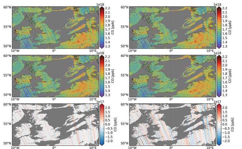
36 CO retrievals of a TROPOMI orbit granule on 27 June 2018 over the UK. Panels of the first
row depict the original data, the second row shows the destriped TROPOMI CO data (FMD
method left, FFD method right), and the third row illustrates the destriping mask that was
subtracted from the original TROPOMI data. . . . . . . . . . . . . . . . . . . . . . . . . . . . . . . . . . . . . . . . . . . . . . . . . . . . . 70
37 Overall structure of the SWIR preprocessor. . . . . . . . . . . . . . . . . . . . . . . . . . . . . . . . . . . . . . . . . . . . . . . . . . . . . 79
38 CH4 error of a non-scattering retrieval from the SWIR 2315–2324 nm spectral window for
a water cloud with optical thickness of 5 as function of cloud height and cloud fraction (left
panel, for more details see generic scenario B in Sec. 7.1) and for a cirrus cloud at 10 km
height as function of surface albedo and cirrus optical thickness (right panel, for more details
see generic scenario E in Sec. 7.1). . . . . . . . . . . . . . . . . . . . . . . . . . . . . . . . . . . . . . . . . . . . . . . . . . . . . . . . . . . . . . 81
39 CH4 two-band cloud filter for the cloud scenarios of Fig. 38. The methane cloud filter relies
on non-scattering methane column retrieval from strong and weak absorption features at
2363-2373 nm and 2310-2315 nm, respectively. . . . . . . . . . . . . . . . . . . . . . . . . . . . . . . . . . . . . . . . . . . . . . . . . 82
40 H2 O two-band cloud filter for the cloud scenarios of Fig. 38. The filter relies on non-scattering
methane column retrieval from strong and weak absorption features at 2367-2377 nm and
2329-2334 nm, respectively. . . . . . . . . . . . . . . . . . . . . . . . . . . . . . . . . . . . . . . . . . . . . . . . . . . . . . . . . . . . . . . . . . . . . . . 82S5P ATBD draft SRON-S5P-LEV2-RP-002
issue 2.2.0, 2021-02-16 – released Page 9 of 82
1 Introduction
1.1 Identification
This document describes the carbon monoxide column retrieval algorithm from Sentinel-5 Precursor (S5P)
measurements in the shortwave infrared (SWIR) spectral range between 2310 and 2340 nm. It is one of the
deliverables of the ESA project ’Sentinel-5 P level 2 processor development’ [AD1].
1.2 Purpose and objectives
The purpose of the document is to describe the theoretical baseline of the algorithm that is used for the
operational processing of the carbon monoxide column densities from S5P measurements in the SWIR spectral
range. Input, output and ancillary data are described. Additionally, the performance of the algorithm is analyzed
with respect to the expected calculation times and the data product uncertainty.
1.3 Document overview
The document is structured as follows: After this introduction, references are provided in Sec. 2 and Sec. 3
contains a list of abbreviations used in this document. Sec. 4 provides a short introduction to satellite remote
sensing of atmospheric CO abundance and the heritage of the presented algorithm is summarized. Moreover,
we recall the level-2 requirement for the CO column product which represents the underlying criterion for the
performance analysis of the presented algorithm. The theoretical concept of the CO retrieval algorithm SICOR
is summarized in Sec. 5, comprising a description of the radiative transfer model and the inversion scheme. The
parameters to be retrieved, ancillary data and a priori knowledge are discussed including the final data product
of the algorithm. Section 7 considers the performance of the retrieval algorithm based on a set of generic
measurement ensembles and a geo-physical ensemble of simulated measurements over China. Here, we
investigate the CO retrieval noise and CO retrieval biases due to forward model errors, erroneous atmospheric
input data and instrument artifacts. Based on this, we evaluate the algorithm performance in the context of
the S5P level-1 and 2 requirements. The numerical feasibility is the subject of Sec. 9, which comprises an
estimate of the numerical effort, a high level data product description and the spatial data selection criteria of
the measurements to be processed. The a posteriori destriping approach that is deployed on the S5P level-2
data product within the operational processing of ESA is introduced in Sec. 10. and Sec. 11 concludes our
document.
Additional material is provided in the appendices, where Appendix A discusses in detail the linearized
two-stream method and Appendix B describes the SWIR preprocessing module which provides required input
to both the SICOR CO algorithm and the RemoTeC CH4 algorithm (see [RD2]).S5P ATBD draft SRON-S5P-LEV2-RP-002
issue 2.2.0, 2021-02-16 – released Page 10 of 82
2 Applicable and reference documents
2.1 Applicable documents
[AD1] Sentinel-5P Level 2 Processor Development – Statement of Work.
source: ESA; ref: S5P-SWESA-GS-053; date: 2012.
[AD2] GMES Sentinels 4 and 5 mission requirements document.
source: ESA; ref: EOP-SMA/1507/JL-dr; date: 2011.
[AD3] GMES Sentinel-5 Precursor – S5p System Requirement Document.
source: ESA; ref: S5p-RS-ESA-SY-0002; date: 2011.
[AD4] NL TROPOMI L2 data processors: Processor Design Document.
source: KNMI; ref: S5P-KNMI-L2-0030-SD; issue: 0.0.0; date: 2014-05-22.
2.2 Standard documents
[SD1] Space Engineering – Software.
source: ESA; ref: ECSS-Q-ST-80C; date: 2009.
[SD2] Space Product Assurance – Software Product Assurance.
source: ESA; ref: ECSS-E-ST-40C; date: 2009.
2.3 Reference documents
[RD1] A. J. Heymsfield and C. M. R. Platt; A Parameterization of the Particle Size Spectrum of Ice Clouds
in Terms of the Ambient Temperature and the Ice Water Content. J. Atmos. Sci.; 41 (1984), 846;
doi:10.1175/1520-0469(1984)0412.0.CO;2.
[RD2] Algorithm Theoretical Baseline Document for Sentinel-5 Precursor methane retrieval.
source: SRON; ref: SRON-S5P-LEV2-RP-001; date: 2014.
[RD3] Terms, definitions and abbreviations for TROPOMI L01b data processor.
source: KNMI; ref: S5P-KNMI-L01B-0004-LI; date: 2011.
[RD4] Terms and symbols in the TROPOMI algorithm team.
source: KNMI; ref: SN-TROPOMI-KNMI-049; date: 2012.
[RD5] H.H. Levy; Normal atmosphere: Large radical and formaldehyde concentrations predicted. Science;
173 (1971), 141.
[RD6] J.A. Logan, M.J. Prather, S.C. Wofsy et al.; Tropospheric chemistry: A global perspective. J. Geophys.
Res.; 86 (1981), 7210.
[RD7] D.T. Shindell, G. Faluvegi, D.S. Stevenson et al.; Multi-model simulations of carbon monoxide: Com-
parison with observations and projected near-future changes. J. Geophys. Res.; 111 (2006), D19306,
doi: 10.1029/2006JD007100.
[RD8] D.P. Edwards, L.K. Emmons, D.A. Hauglustaine et al.; Observations of carbon monoxide and aerosols
from the Terra satellite: Northern Hemisphere variability. J. Geophys. Res.; 109 (2004), D24202, doi:
10.1029/2004JD004727.
[RD9] A.M.S. Gloudemans, M.C. Krol, J.F. Meirink et al.; Evidence for long-range transport of Carbon
Monoxide in the Southern Hemisphere from SCIAMACHY observations. Geophys. Res. Lett.; 33
(2006), L16807, doi:10.1029/2006GL026804.
[RD10] Antje Inness, Melanie Ades, Anna Agusti-Panareda et al.; The CAMS reanalysis of atmospheric
composition. Atmospheric Chemistry and Physics; 19 (2019), 3515; doi:10.5194/acp-19-3515-2019.
[RD11] A. Hollingsworth, R. J. Engelen, A. Benedetti et al.; Toward a Monitoring and Forecasting System For
Atmospheric Composition: The GEMS Project. Bull. Amer. Meteor. Soc.; 89 (2008), 1147.S5P ATBD draft SRON-S5P-LEV2-RP-002
issue 2.2.0, 2021-02-16 – released Page 11 of 82
[RD12] H.G. Reichle Jr and V.S. Connors; The mass of CO in the atmosphere during October 1984, April
1994, and October 1994. J. Atmos. Sci.; 56 (1999), 307.
[RD13] H. Kobayashi, A. Shimota, K. Kondo et al.; Development and evaluation of the Interferometric Monitor
for Greenhouse Gases: a high throughput Fourier transform infrared radiometer for nadir Earth
observations. Appl. Opt.; 38 (1999), 6801.
[RD14] M.N. Deeter, L. K. Emmons, G. L. Francis et al.; Operational carbon monoxide retrieval al-
gorithm and selected results for the MOPITT instrument. J. Geophys. Res.; 108 (2003), 4399,
doi:10.1029/2002JD003186.
[RD15] W.W. McMillan, C. Barnet, L. Strow et al.; Daily global maps of carbon monoxide from NASA’s
Atmospheric Infrared Sounder. Geophys. Res. Lett.; 32 (2005), L11801, doi:10.1029/2004GL021821.
[RD16] C. P. Rinsland, M. Luo, J. A. Logan et al.; Nadir measurements of carbon monoxide distributions
by the Tropospheric Emission Spectrometer instrument onboard the Aura Spacecraft: Overview
of analysis approach and examples of initial results. Geophys. Res. Lett.; 33 (2006), L22806,
doi:10.1029/2006GL027000.
[RD17] S. Turquety, J. Hadji-Lazaro, C. Clerbaux et al.; Operational trace gas retrieval algorithm for
the Infrared Atmospheric Sounding Interferometer. J. Geophys. Res.; 109 (2004), D21301,
doi:10.1029/2004JD004821.
[RD18] The potential of MTG-IRS and S4-TIR to detect high pollution events at urban and regional scales.
source: EUMETSAT; ref: EUM/CO/07/4600000447/SAT; date: 2009.
[RD19] H. Bovensmann, J. P. Burrows, M. Buchwitz et al.; SCIAMACHY: Mission Objectives and Measurement
Modes. Journal of Atmospheric Sciences; 56 (1999), 127.
[RD20] M.N. Deeter, D. P. Edwards, J. C. Gille et al.; CO retrievals based on MOPITT near-infrared observations.
J. Geophys. Res.; 114 (2009), D04303, doi:10.1029/2008JD010872.
[RD21] H. M. Worden, M. N. Deeter, D. P. Edwards et al.; Observations of near-surface carbon monox-
ide from space using MOPITT multispectral retrievals. J. Geophys. Res.; 115 (2010), D18314,
doi:10.1029/2010JD014242.
[RD22] P. Veefkind; TROPOMI on the ESA Sentinel-5 Precursor: a GMES mission for Global Observations of
the Atmospheric Composition for Climate and Air Quality Applications. Remote Sens. Envirom.; 120
(2012), 70.
[RD23] M. Buchwitz, I. Khlystova, H. Bovensmann et al.; Three years of global carbon monoxide from
SCIAMACHY: comparison with MOPITT and first results related to the detection of enhanced CO over
cities. Atmos. Chem. Phys.; 7 (2007), 2399.
[RD24] C Frankenberg, U. Platt and T. Wagner; Retrieval of CO from SCIAMACHY onboard ENVISAT:
detection of strongly polluted areas and seasonal patterns in global CO abundances. Atmos. Chem.
Phys.; 4 (2005), 8425.
[RD25] A.M.S. Gloudemans, A.T.J. de Laat, H. Schrijver et al.; SCIAMACHY CO over land and oceans:
2003-2007 interannual variability. Atmos. Chem. Phys.; 9 (2009), 3799.
[RD26] M. Buchwitz, R. de Beek, S. Noel et al.; Atmospheric carbon gases retrieved from SCIAMACHY by
WFM-DOAS: version 0.5 CO and CH4 and impact of calibration improvements on CO2 retrieval. Atmos.
Chem. Phys.; 6 (2006), 2727.
[RD27] S. Turquety, C. Clerbaux, K. Law et al.; CO emission and export from Asia: an analysis combining
complementary satellite measurements (MOPITT, SCIAMACHY and ACE-FTS) with global modeling.
Atmos. Chem. Phys.; 8 (2008) (17), 5187.
[RD28] A. T. J. de Laat, A. M. S. Gloudemans, I. Aben et al.; Global evaluation of SCIAMACHY and MO-
PITT carbon monoxide column differences for 2004-2005. J. Geophys. Res.; 115 (2010), D06307,
doi:10.1029/2009JD012698.S5P ATBD draft SRON-S5P-LEV2-RP-002
issue 2.2.0, 2021-02-16 – released Page 12 of 82
[RD29] B. Dils, M. De Maziere, J. F. Muller et al.; Comparisons between SCIAMACHY and ground-based FTIR
data for total columns of CO, CH4 , CO2 and N2 O. Atmos. Chem. Phys.; 6 (2006), 1953.
[RD30] A. T. J. de Laat, A. M. S. Gloudemans, H. Schrijver et al.; Validation of five years (2003-2007) of
SCIAMACHY CO total column measurements using ground-based spectrometer observations. Atmos.
Meas. Tech.; 3 (2010), 1457.
[RD31] A. T. J. de Laat, A. M. S. Gloudemans, I. Aben et al.; Scanning Imaging Absorption Spectroscopy for
Atmospheric Chartography carbon monoxide total columns: Statistical evaluation and comparison with
chemistry transprot model results. J. Geophys. Res.; 112 (2007), D12310, doi:10.1029/2006JD008256.
[RD32] GMES Sentinels 4 and 5 mission requirements document.
source: ESA; ref: EOP-SMA/1507/JL-dr; date: 2011.
[RD33] J. Vidot, J. Landgraf, O.P. Hasekamp et al.; Carbon monoxide from shortwave infrared reflectance
measurements: A new retrieval approach for clear sky and partially cloudy atmospheres. Remote
Sens. Envirom.; 120 (2012), 255.
[RD34] M. Krol, S. Houweling, B. Bregman et al.; The two-way nested global chemistry-transport zoom model
TM5: algorithm and applications. Atmos. Chem. Phys.; 5(2) (2005), 417.
[RD35] C.D. Rodgers; Inverse Methods for Atmospheres: Theory and Practice; volume 2 (World Scientific,
2000).
[RD36] A.M.S. Gloudemans, H. Schrijver, O.P. Hasekamp et al.; Error analysis for CO and CH4 total column
retrieval from SCIAMACHY 2.3µm spectra. Atmos. Chem. Phys.; 8 (2008), 3999.
[RD37] W.G. Zdunkowski, Welch R.M. and Korb G.; An Investigation of the Structure of Typical Two-stream-
methods for the Calculation of Solar Fluxes and Heating Rates in Clouds. Contrib. Atmos. Phys.; 53
(1979), 147.
[RD38] W. J. Wiscombe and G. W. Grams; The backscattered fraction in two-stream approximations. Journal
of Atmospheric Sciences; 33 (1976), 2440.
[RD39] G.I. Marchuk; Equation for the Value of Information from Weather Satellites and Formulation of Inverse
Problems. Cosmic Res.; 2 (1964), 394.
[RD40] M.A. Box, S.A.W. Gerstl and C. Simmer; Application of the adjoint formulation to the calculation of
atmospheric radiative effects. Beitr. Phys. Atmos.; 61 (1988), 303.
[RD41] J. Landgraf, O.P. Hasekamp, M. Box et al.; A Linearized Radiative Transfer Model Using the Analytical
Perturbation Approach. J. Geophys. Res.; 106 (2001), 27291.
[RD42] O.P. Hasekamp and J. Landgraf; A linearized vector radiative transfer model for atmospheric trace gas
retrieval. J. Quant. Spectrosc. Radiat. Transfer; 75 (2002).
[RD43] V.V. Rozanov, D. Diebel, R.J.D. Spurr et al.; GOMETRAN: A radiative transfer model for the satellite
project GOME, the plan-parallel version. J. Geophys. Res.; 102 (1997), 16,683.
[RD44] V.V. Rozanov, T. Kurosu and J.P. Burrows; Retrieval of Atmospheric Constituents in the UV-Visible:
A new Quasi-Analytical Approach for the Calculation of Weighting Functions. J. Quant. Spectrosc.
Radiat. Transfer; 60 (1998), 277.
[RD45] H. H. Walter, J. Landgraf and O. P. Hasekamp; Linearization of a pseudo-spherical vector radiative
transfer model. J. Quant. Spectrosc. Radiat. Transfer; 85 (2004), 251.
[RD46] H. H. Walter and J. Landgraf; Towards linearization of atmospheric radiative transfer in spherical
geometry. J. Quant. Spectrosc. Radiat. Transfer; 95 (2005), 175.
[RD47] H. H. Walter, J. Landgraf, F. Spada et al.; Linearization of a radiative transfer model in spherical
geometry. J. Geophys. Res.; 111 (2006), 10.1029/2005JD007014.
[RD48] G. I. Bell and S. Glasstone; Nuclear Reactor Theory (Van Nostrand Reinhold Company, New York,
1970).S5P ATBD draft SRON-S5P-LEV2-RP-002
issue 2.2.0, 2021-02-16 – released Page 13 of 82
[RD49] J. Lewins; Importance, the adjoint function (Pergamon Press, Oxford, England, 1965).
[RD50] E. A. Ustinov; Inverse problem of photometric observation of solar radiation reflected by an optically
dense planetary atmosphere. Mathematical methods and weighting functions of linearized inverse
problem. Cosmic Res.; 29 (1991), 519.
[RD51] P.L. Phillips; A technique for the numerical solution of certain integral equations of the first kind. J. Ass.
Comput. Mat.; 9 (1962), 84.
[RD52] A.N. Tikhonov; On the solution of incorrectly stated problems and a method of regularization. Dokl.
Acad. Nauk SSSR; 151 (1963), 501.
[RD53] P.C. Hansen; Analysis of discrete ill posed problems by means of the L-curve. SIAM Rev.; 34 (1992),
561.
[RD54] P.C. Hansen and D.P. O’Leary; The use of the L-curve in the regularization of discrete ill posed
problems. SIAM J. Sci. Comput.; 14 (1993), 1487.
[RD55] T. Borsdorff, O. P. Hasekamp, A. Wassmann et al.; Insights into Tikhonov regularization: application to
trace gas column retrieval and the efficient calculation of total column averaging kernels. Atmospheric
Measurement Techniques; 7 (2014) (2), 523; doi:10.5194/amt-7-523-2014. URL https://doi.org/
10.5194/amt-7-523-2014.
[RD56] A. Butz, A Galli, O.P. Hasekamp et al.; ROPOMI aboard Sentinel-5 Precursor: Prospective performance
of CH4 retrievals for aerosol and cirrus loaded atmospheres. Remote Sens. Envirom.; 120 (2012), 267.
[RD57] W.H. Press, S.A. Teukolsky, W.T. Vetterling et al.; Numerical Recipes in C: The Art of Scientific
Computing (Cambridge University Press, 1992); 2nd edition.
[RD58] M. Birk., G. Wagner, J. Loos et al.; Methane and water spectroscopic database for TROPOMI Sentinel
5 Precursor in the 2.3µm region. volume 19; (p. 4652) (EGU General Assembly, 2017).
[RD59] SEOM-IAS validation report.
source: DLR; ref: IAS-D09-PRJ-066.
[RD60] T. Borsdorff, J. aan de Brugh, A. Schneider et al.; Improving the TROPOMI CO data product: update of
the spectroscopic database and destriping of single orbits. Atmospheric Measurement Techniques; 12
(2019) (10), 5443; doi:10.5194/amt-12-5443-2019. URL https://amt.copernicus.org/articles/
12/5443/2019/.
[RD61] T. Borsdorff, J. aan de Brugh, H. Hu et al.; Mapping carbon monoxide pollution from space down to city
scales with daily global coverage. Atmospheric Measurement Techniques Discussions; 2018 (2018), 1;
doi:10.5194/amt-2018-132. URL https://www.atmos-meas-tech-discuss.net/amt-2018-132/.
[RD62] OMI aerosol retrieval algorithm.
source: KNMI; ref: ATBD-OMI-03; date: 2001.
[RD63] J.M.J. Schepers, D.and aan de Brugh, Ph. Hahne, A. Butz et al.; LINTRAN v2.0: A linearised vector
radiative transfer model for efficient simulation of satellite-born nadir-viewing reflection measurements
of cloudy atmospheres. J. Quant. Spectrosc. Radiat. Transfer; 149 (2015), 247.
[RD64] S. Chandrasekhar; Radiative transfer (Dover Publications, Inc., New York, 1960).
[RD65] M. Hess and M. Wiegner; COP: a data library of optical properties of hexagonal ice crystals. Appl.
Opt.; 33 (1994) (33), 7740; doi:10.1364/AO.33.007740.
[RD66] M. Hess, R. B. A. Koelemeijer and P. Stammes; Scattering matrices of imperfect hexagonal ice
crystals. Journal of Quantitative Spectroscopy and Radiative Transfer; 60 (1998), 301 ; doi:DOI:
10.1016/S0022-4073(98)00007-7.
[RD67] A Marshak, A. Davis, W. Wiscombe et al.; The Verisimilitude of the Independent Pixel Approximation
Used in Cloud Remote Sensing. Remote Sens. Envirom.; 52 (1995), 71.S5P ATBD draft SRON-S5P-LEV2-RP-002
issue 2.2.0, 2021-02-16 – released Page 14 of 82
[RD68] Instrument noise model for the Sentinel 5 SWIR bands.
source: Netherlands Insitute for Space Research, SRON; ref: SRON-TROPSC-TN-2011-002; date:
2011.
[RD69] U.S. Standard Atmosphere, 1976.
source: National Oceanic and Atmospheric Administration; ref: NOAA-S/T76-1562.
[RD70] Observation Techniques and Mission Concepts for Atmospheric Chemistry (CAMELOT).
source: European Space Agency; ref: 20533/07NL/HE.
[RD71] A. E. Dessler and P. Yang; The Distribution of Tropical Thin Cirrus Clouds Inferred from Terra MODIS
Data. Journal of Climate; 16 (2003), 1241.
[RD72] P. Yang, B.-C. Gao, B.A. Baum et al.; Radiative properties of cirrus clouds in the infrared (8–13 µm)
spectral region. J. Quant. Spectrosc. Radiat. Transfer; (2001).
[RD73] B. Mijling and R.J. van der A; Using daily satellite observations to estimate emissions of short-lived air
pollutants on a mesoscopic scale. J. Geophys. Res.; (2012).
[RD74] T.P.C. van Noije, H.J. Eskes, F.J. Dentener et al.; Multi-model ensemble simulations of tropospheric
NO2 compared with GOME retrievals for the year 2000. Atmos. Chem. Phys.; 6 (2006), 2943.
[RD75] J. F. Meirink, P. Bergamaschi and M. C. Krol; Four-dimensional variational data assimilation for inverse
modelling of atmospheric methane emissions: Method and comparison with synthesis inversion.
Atmos. Chem. Phys.; 8 (2008), 6341.
[RD76] P. Bergamaschi, M. Krol, F. Dentener et al.; Inverse modelling of national and european CH4 emissions
using the atmospheric zoom model TM5. Atmos. Chem. Phys.; 5 (2005), 2431.
[RD77] P. Bergamaschi, C. Frankenberg, J.-F. Meirink et al.; Inverse modeling of global and re-
gional CH4 emissions using SCIAMACHY satellite retrievals. J. Geophys. Res.; 114 (2009),
doi:10.1029/2009JD012287.
[RD78] A. Butz, S. Guerlet, O. Hasekamp et al.; Toward accurate CO2 and CH4 observations from GOSAT.
Geophys. Res. Lett.; 38 (2011), doi:10.1029/2011GL047888.
[RD79] Sentinel-5 precursor/TROPOMI: Level 2 Product User Manual Carbon Monoxide.
source: SRON; ref: SRON-S5P-LEV2-MA-002; issue: 0.8.1; date: 2015-012-08.
[RD80] K. F. Boersma, H. J. Eskes, R. J. Dirksen et al.; An improved tropospheric NO2 column retrieval
algorithm for the Ozone Monitoring Instrument. Atmospheric Measurement Techniques; 4 (2011) (9),
1905; doi:10.5194/amt-4-1905-2011. URL https://www.atmos-meas-tech.net/4/1905/2011/.
[RD81] T. Borsdorff, J. aan de Brugh, S. Pandey et al.; Carbon monoxide air pollution on sub-city scales and
along arterial roads detected by the Tropospheric Monitoring Instrument. Atmospheric Chemistry and
Physics; 19 (2019) (6), 3579; doi:10.5194/acp-19-3579-2019. URL https://www.atmos-chem-phys.
net/19/3579/2019/.
[RD82] T. Borsdorff, A. García Reynoso, G. Maldonado et al.; Monitoring CO emissions of the met-
ropolis Mexico City using TROPOMI CO observations. Atmospheric Chemistry and Physics;
20 (2020) (24), 15761; doi:10.5194/acp-20-15761-2020. URL https://acp.copernicus.org/
articles/20/15761/2020/.
[RD83] F. Kasten and T. Young; Revised optical air mass tables and approximation formula. Appl. Opt.; 28
(1989), 4735.
2.4 Electronic references
There are no electronic referencesS5P ATBD draft SRON-S5P-LEV2-RP-002 issue 2.2.0, 2021-02-16 – released Page 15 of 82 3 Terms, definitions and abbreviated terms Terms, definitions and abbreviated terms that are used in the development program for the TROPOMI L0 1b data processor are described in [RD3]. Terms, definitions and abbreviated terms that are used in development program for the TROPOMI L2 data processors are described in [RD4]. Terms, definitions and abbreviated terms that are specific for this document can be found below.
S5P ATBD draft                                                                 SRON-S5P-LEV2-RP-002
issue 2.2.0, 2021-02-16 – released                                                      Page 16 of 82

3.1     Acronyms and abbreviations
 ADEOS                 Advanced Earth Observing System
 AIRS                  Atmospheric Infrared Sounder
 AOT                   Aerosol Optical Thickness
 AQUA                  A NASA Earth Science satellite mission focussing on the Earth’s water cycle
 CTM                   Chemical Transport Model
 DFS                   Degree of Freedom for Signal
 S-LINTRAN             Scalar linearised Radiative Transfer Program for a Multi-Layered Plane-Parallel Medium
 ECMWF                 European Centre for Medium-Range Weather Forecasts
 ERI                   European Research Institute
 ESRL                  Earth System Research Laboratory
 FFD                   Fourier filter destriping
 FFM                   Fixed mask destriping
 FTS                   Fourier Transform Spectrometer
 FTIR                  Fourier Transform Infrared
 FRESCO                Fast Retrieval Scheme for Clouds from the Oxygen A band
 FWHM                  Full Width Half Maximum
 GCM                   General Circulation Model
 GMES                  Global Monitoring for Environment and Security
 GNIP                  Global Network for Isotopes in Precipitation
 GOSAT                 Greenhouse gases Observing Satellite
 IAGOS                 In-service Aircraft for a Global Observing System
 IASI                  Infrared Atmospheric Sounding Interferometer
 IMAP                  Iterative Maximum A Posteriori
 IMG                   Interferometric Monitor for Greenhouse gases
 IMLM                  Iterative Maximum Likelihood Method
 IRWG                  Infrared Working Group
 ISRF                  Instrument Spectral Response Function
 L1                    Level-1
 L2                    Level-2
 LER                   Lambert-equivalent Reflectivity
 LOS                   Line of Sight
 MACC                  Monitoring Atmospheric Composition and Climate
 MAPS                  Measurement of Air Pollution from Satellites
 MODIS                 Moderate Resolution Imaging Spectroradiometer
 MOPITT                Measurements of Pollution in the Troposphere
 MOZAIC                Measurement of Ozone and Water Vapour on Airbus in-service Aircraft
 NDACC                 Network for the Detection of Atmospheric Composition Change
 NOAA                  National Oceanic and Atmospheric Administration
 NPP                   National Polar-orbiting Partnership
 NRT                   Near Real Time
 OMI                   Ozone Monitoring Instrument
 PIFM                  Practical Improved Flux Method
 RemoTeC               Remote Sensing of Greenhouse Gases for Carbon Cycle Modelling
 RMS                   Root Mean Square
S5P ATBD draft                                                                 SRON-S5P-LEV2-RP-002
issue 2.2.0, 2021-02-16 – released                                                      Page 17 of 82

    S5P                    Sentinel-5 Precursor
    SCIAMACHY              Scanning Imaging Absorption Spectrometer for Atmospheric Chartography
    SEOM-IAS               Scientific Exploitation of Operational Missions - Improved Atmospheric Spectroscopy
                           Databases
    SICOR                  Shortwave Infrared CO Retrieval
    SMOW                   Standard Mean Ocean Water
    SNR                    Signal-to-Noise Ratio
    SPEC                   Standard Performance Evaluation Corporation
    SSD                    Spectral Sampling Distance
    SWIR                   Shortwave Infrared
    SZA                    Solar Zenith Angle
    TCCON                  Total Carbon Column Observing Network
    TES                    Tropospheric Emission Spectrometer
    TM4                    Transport Model 4
    TM5                    Transport Model 5
    TOA                    Top Of model Atmosphere
    TROPOMI                Tropospheric Monitoring Instrument
    VIIRS                  Visible Infrared Imager Radiometer Suite
    VZA                    Viewing Zenith Angle
    WFM-DOAS               Weighting Function Modified-Differential Optical Absorption Spectroscopy
S5P ATBD draft SRON-S5P-LEV2-RP-002
issue 2.2.0, 2021-02-16 – released Page 18 of 82
4 Remote Sensing of Carbon Monoxide
Carbon monoxide (CO) is an important atmospheric trace gas and in certain urban areas, it is a major
atmospheric pollutant. Measurements of its global abundance improve our understanding of tropospheric
chemistry and atmospheric long range transport [RD5, RD6, RD7, RD8]. Main sources of CO are combustion
of fossil fuels, biomass burning, and atmospheric oxidation of methane and other hydrocarbons. Whereas fossil
fuel combustion is the main source of CO at Northern mid-latitudes, the oxidation of isoprenes and biomass
burning play an important role in the tropics. Due to the long lifetime of methane (CH4 ), its oxidation provides a
close-to uniform background on the global CO distribution. The most important sink of CO is its reaction with
the hydroxyl radical OH. The CO lifetime is several weeks to several months, which makes CO a good tracer
to study long range transport processes (e.g. [RD9]). Moreover, CO is one of the highest priority chemical
species measured by the Copernicus Atmosphere Monitoring Service (CAMS) project [RD10, RD11].
The first spaceborne measurements of CO were performed with the MAPS (Measurement of Air Pollution
from Satellites) instrument during four flights of the space shuttle between 1981 and 1999 [RD12], and with the
IMG (Interferometric Monitor for Greenhouse gases) instrument onboard ADEOS (Advanced Earth Observing
System) in 1996 and 1997 [RD13]. Since 2000, long-term global data sets of CO are provided by MOPITT
(Measurements of Pollution in the Troposphere) instrument (e.g. [RD14]), which measures in two spectral
ranges at 2.3 µm and 4.7 µm, respectively, using correlation radiometry. At present, the operational CO
MOPITT data product relies only on measurements around the fundamental 1-0 CO absorption band at
4.7 µm. This spectral range is also employed by three other spaceborne spectrometers which measure
the infrared brightness of the Earth’s surface and the atmosphere: (1) AIRS (Atmospheric Infrared Sounder
[RD15]) launched in 2002 onboard the Aqua satellite, (2) TES (Tropospheric Emission Spectrometer [RD16]
launched in 2004 onboard the Aura satellite and (3) IASI (Infrared Atmospheric Sounding Interferometer[RD17])
onboard a series of three METOP (Meteorological Operational) satellites. Generally, these thermal infrared
measurements exhibit peak sensitivity to CO in the middle troposphere and are thus well suited to study long
range atmospheric transport. However, depending on spectral resolution and the thermal contrast in the lower
troposphere, the measurements show also sensitivity to CO in the lower troposphere [RD18].
CO total columns with sensitivity to the tropospheric boundary layer can be inferred from sunlight reflected
by the Earth atmosphere in the 2.3 µm spectral range of the shortwave infrared (SWIR) part of the solar
spectrum. The first overtone 2-0 absorption band of CO is situated between 2305 nm and 2385 nm. For clear
sky measurements, this spectral range is subject to little atmospheric scattering and most of the measured light
is thus reflected by the Earth’s surface. SWIR measurements are therefore sensitive to the integrated amount
of CO along the light path, including the contribution of the planetary boundary layer. This makes the SWIR
spectral range particularly suitable for detecting surface sources of CO. Since the launch of SCIAMACHY
(Scanning Imaging Absorption Spectrometer for Atmospheric Chartography [RD19] in the year 2002 on the
Envisat satellite, a continuous time series of global CO SWIR measurements is available. Moreover, first results
were reported recently using MOPITT measurements in the SWIR [RD20] and a combination of SWIR and
the 4.7 µm CO absorption band [RD21]. However, new space-borne instrumentation is required to ensure
continuity of SWIR measurements of CO in the future. In this respect, the Sentinel 5 Precursor mission (S5P
[RD22]) provides the opportunity to extend this unique long-term global data set of CO using the same type of
measurement. On top of that, the major scientific objective of these mission is to participate in the development
and improvement of air quality model processes and data assimilation in support of operational services,
including air quality forecasting and protocol monitoring. This scientific objective requires the combination of
new instrumentation with better radiometric performances and higher spatial sampling, and the development of
fast and accurate retrieval algorithms.
4.1 Algorithm heritage
Several fast algorithms are used to retrieve CO column from SCIAMACHY SWIR measurements, including the
Weighting Function Modified-Differential Optical Absorption Spectroscopy (WFM-DOAS) approach ([RD23] and
references therein) the Iterative Maximum A Posteriori (IMAP) approach [RD24], and the Iterative Maximum
Likelihood Method (IMLM) approach ([RD25], and references therein). These algorithms retrieve vertically
integrated CO column density over land and above clouds over oceans. Over ocean, the surface albedo
is too low to retrieve CO under clear sky conditions. For numerical efficiency, scattering by aerosols and
clouds is not considered in the radiative transfer of the IMLM retrieval approach. Both Buchwitz et al. [RD26]
and Gloudemans et al. [RD25] use a priori methane information to characterise the light path through the
atmosphere. The different approaches allow the detection of strongly polluted areas, the seasonal variability
of global atmospheric CO and the long range transport of CO. The retrievals have been compared withS5P ATBD draft SRON-S5P-LEV2-RP-002
issue 2.2.0, 2021-02-16 – released Page 19 of 82
chemical transport models (CTM, e.g. [RD27, RD25]), with MOPITT retrievals (e.g. [RD23, RD28]) and
ground-based FTIR (Fourier Transform Infrared) measurements [RD29, RD30]. Since CO is a weak absorber
and SCIAMACHY exhibits a low signal-to-noise ratio in the 2.3 µm region, the retrieval of single-sounding
CO column density is subject to large retrieval noise, typically on the order of 10-100 % [RD31]. Hence, to
compare SCIAMACHY retrievals with ground-based measurements, the averaging of multiple SCIAMACHY
measurements is needed. De Laat et al. [RD30] demonstrated that, at the Northern latitudes and for a typical
sampling area of 8o × 8o , the absolute difference between the mean IMLM SCIAMACHY CO retrievals and
ground-based measurements are close to or fall within the 2σ precision of 2 × 10¹⁷ molec./cm2 . Thus on the
Northern Hemisphere, SCIAMACHY can observe CO adequately for the given sampling size. At mid to high
latitudes of the Southern Hemisphere, the IMLM algorithm systematically underestimates the ground based
measurements by 1 − 5 × 10¹⁷ molec./cm2 . Reasons for this bias are currently under investigation. Next to the
large sampling areas and the Southern Hemisphere bias, one major limitation of the current SWIR CO retrieval
product is that for the individual soundings, no information is provided on the vertical sensitivity of the CO
column retrieval, the so-called column averaging kernel. Column averaging kernels are essential information to
validate SWIR CO retrievals with other independent retrievals or CTM simulations. Last but not least, it is also
an important piece of information for data assimilation in air quality forecasting employing variational schemes.
Based on SCIAMACHY heritage, we present a modified SWIR CO retrieval (SICOR) approach for S5P,
which can be applied to clear sky observations over land and cloudy observations over both land and oceans.
The algorithm is based on the heritage of the CO retrieval algorithm for SCIAMACHY [RD25] but improves
current CO retrieval approaches for cloudy and aerosol loaded atmospheres. A typical SWIR spectrum is
illustrated on the top panel of Fig. 1. It shows the total transmittance of solar light along its path from the Sun
to the surface to the satellite. The transmittance is simulated using the Beer’s extinction law. In the band, the
relevant absorbing species are H2 O, CO and CH4 , with the optical depth of CO generally much smaller than
those of H2 O and CH4 .
Clouds and aerosols affect the sensitivity of the measurement to CO in several manners: due to multiple
scattering, the path length of the observed light is enhanced in the upper part of clouds. For larger optical depth
the scattering layer transmits only a small fraction of incoming light and thus the atmosphere below the layer is
effectively shielded. Furthermore, light can be trapped between a scattering layer and a bright surface, which
can enhance significantly the light path. The developed SICOR algorithm accounts for these effects, but also
takes into consideration the computational aspects of an operational data processing. An accurate treatment
of clouds and aerosols in the retrieval requires the simulation of multiple light scattering which is numerically
very demanding. Therefore, we employ a two-stream radiative transfer solver, which accounts for atmospheric
scattering in a simplified way. Since three decades, different two-stream methods are used to describe radiative
transfer in global chemistry and climate models and they are known to be stable and numerically efficient. We
adapt this method for satellite remote sensing including the linearisation of the model with respect to scattering
and absorption properties in the model atmosphere. In summary, the presented SICOR algorithm builds on
strong heritage of SCIAMACHY CO column retrieval and radiative transfer experience of the last 30 years and
additionally adds new features to the retrieval to fully exploit the potential of TROPOMI SWIR measurement for
an operational data processing.
4.2 Carbon Monoxide level-2 requirements
To improve our present knowledge on CO on a global scale, satellite measurements of the total CO column are
needed within an accuracy of < 15% and a precision with ≤ 10 % even for background CO abundance and low
surface reflection in the shortwave infrared spectral range [RD22, RD32]. For the CO error budget, we assume
that instrument and forward model errors contribute equally to the error budget and that all error terms add up
quadratically. Herewith, both instrument and forward model errors must not exceed 8 %. These CO level-2
requirements should be considered as thresholds.S5P ATBD draft SRON-S5P-LEV2-RP-002 issue 2.2.0, 2021-02-16 – released Page 20 of 82 Figure 1: SWIR spectral transmittance along the light path of the solar beam reflected by the Earth surface into the instrument viewing direction. Simulations are performed for viewing zenith angle (VZA) = 0◦ , and a solar zenith angle (SZA) = 30◦ , and by assuming a US standard atmospheric profile. From top to bottom, the figure shows the total transmittance, the individual transmittances due to H2 O, CH4 , and CO, respectively. Note the different y-axis scale for CO transmittance.
S5P ATBD draft                                                                       SRON-S5P-LEV2-RP-002
issue 2.2.0, 2021-02-16 – released                                                            Page 21 of 82

5     Algorithm Description
To retrieve atmospheric CO abundances from TROPOMI SWIR measurements as a near real-time (NRT) data
product, we follow an algorithm concept which is summarised in Fig. 2. It is a further development of the
retrieval method of Vidot et al. [RD33] and it includes a significant improvement with respect to the description
of atmospheric scattering. The retrieval algorithm requires several input fields:
    • The measured Earth radiance and solar irradiance spectra including noise estimate, solar and viewing
      geometry, and information of geo-location.

    • ECMWF temperature, water vapor and pressure profiles and geo-potential height.

    • An estimate of the CH4 field using a chemistry transport model, e.g. Transport Model 5 (TM5, [RD34]).

    • An estimate of the CO column from a chemistry transport model (e.g. TM5).
The retrieval is performed in two steps: first as part of the SWIR preprocessing module (see Appendix B), the
vertically integrated amount of methane is retrieved from a dedicated fit window of the SWIR band between
2315 and 2324 nm using a non-scattering radiative transfer model. The extent of lightpath shortening and
enhancement due to atmospheric scattering by clouds and aerosols can be indicated by comparing the retrieved
CH4 column with a priori knowledge. If the difference ∆CH4 exceeds a certain threshold, observations are
strongly contaminated by clouds and are rejected. In a second step, the SICOR full physics retrieval approach
is used to infer CO columns from the adjacent spectral window, 2324-2338 nm. Here, the methane absorption
features are used to infer information on atmospheric scattering by clouds and aerosols, which passed the
cloud filter, together with the atmospheric CO and H2 O abundances, surface albedo and a spectral calibration
of the reflectance spectrum. The scattering layer has a triangular height distribution of fixed geometrical
thickness, and its optical depth and height are parameters to be retrieved. This step of the retrieval relies on
accurate a priori knowledge of CH4 which will be provided within an accuracy of ±3 % by a dedicated methane
forecast using the TM5 atmospheric transport model. The atmospheric scattering is described by a two-stream
radiative transfer model. Finally, the retrieval product consists of a CO column estimate including a column
averaging kernel and a random error estimate. A detailed description of input and output fields are given in
Sec. 9.
    For both retrieval approaches, the non-scattering and the scattering retrieval, a forward model F is needed
which describes the measurement as a function of the state of the atmosphere, namely

      y = F(x, b) + ey .                                                                                      (1)

Here, vector y has the spectral measurements as its components, state vector x represents the parameters to
be retrieved, b describes parameters other than the state vector that influences the measurement, and ey is the
error of the measurement. For the retrieval of CO from SWIR measurements, the forward model is non-linear in
the state vector x. Therefore, the inversion problem is solved iteratively employing the Gauss-Newton method,
where for each iteration step the forward model is linearized by a Taylor expansion around the solution of the
previous iteration xo ,

                                ∂F
      F(x, b) = F(xo , b) +        (xo , b){x − xo } + O(x2 ) ,                                               (2)
                                ∂x
where O(x2 ) indicates second and higher order contributions of the expansion. This iteration approach shows
satisfying convergence properties for moderately non-linear problems [RD35]. In the following sub-sections,
both the SICOR inversion approach and the forward model are described in more depth.

5.1   Forward model
We assume that the measurement vector y contains the spectral reflectance ri sampled at spectral points
λi as its components. The forward model F simulates the measurement by a spectral convolution of both
the top-of-model-atmosphere (TOA) radiance and the solar irradiance with the instrument spectral response
function (ISRF),

                            Z
      IiTOA = s ∗ I TOA =        s(λi , λ) I TOA (λ)dλ ,                                                      (3)
You can also read