THE GRAPH MATCHING AND QUADRATIC ASSIGNMENT PROBLEMS
←
→
Page content transcription
If your browser does not render page correctly, please read the page content below

THE GRAPH MATCHING AND
 QUADRATIC ASSIGNMENT
       PROBLEMS

                          by

                   Ali Saad-Eldin

  A thesis submitted to Johns Hopkins University

in conformity with the requirements for the degree of
          Master of Science in Engineering

                Baltimore, Maryland

                      May 2021

                © 2021 Ali Saad-Eldin

                  All rights reserved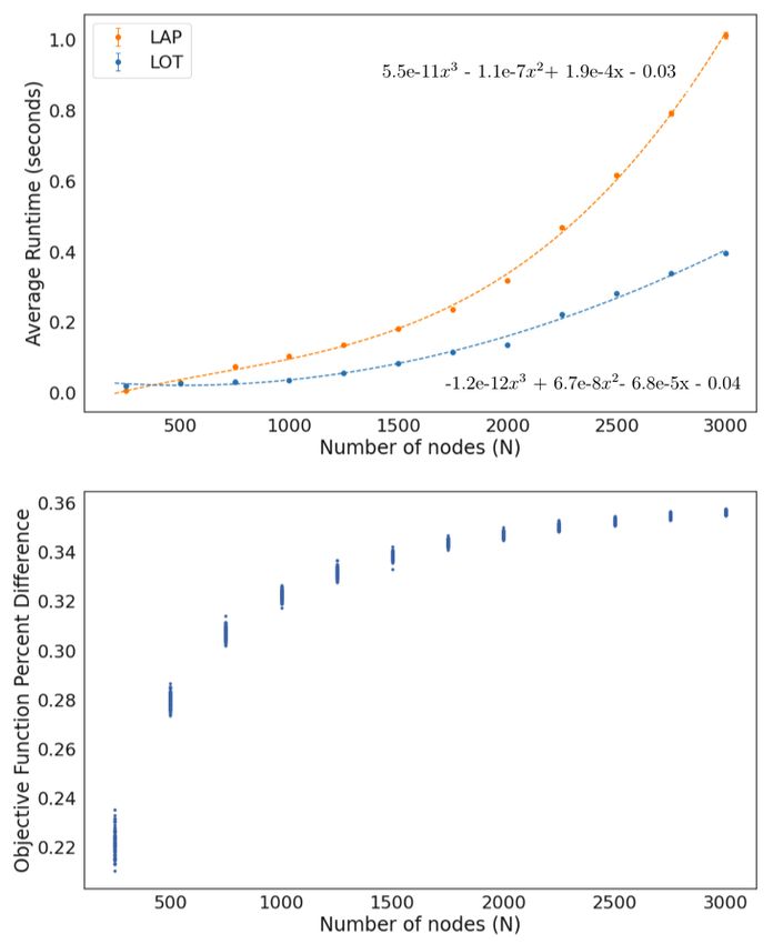
Abstract

The graph matching problem seeks to find an alignment between the nodes of

two graphs that minimizes the number of edge disagreements. We present
a modification to the state-of-the-art graph matching approximation algo-
rithm "FAQ" (Vogelstein, 2015), replacing it’s linear sum assignment step with

the "Lightspeed Optimal Transport" method of Cuturi (2013). The modifi-
cation provides a speed improvement by replacing the main computational
bottleneck, as well as robustness to stochasticity between graph pairs. The

effectiveness of the approach is demonstrated in matching graphs in simulated
and real data examples.

Primary Reader and Advisor: Professor Joshua Vogelstein
Secondary Reader: Professor Carey Priebe

                                      ii
Acknowledgments
First, I would like to thank my advisor Joshua Vogelstein for his continued
mentorship and support of the work presented, and for allowing me the
opportunity to pursue my research interests. This work would not be possible
without his guidance. I’d also like to thank Carey Priebe, whose enthusiasm
and curiosity for math is contagious. He taught me what it meant to be excited
about ones work.
I would like to thank the members of the NeuroData lab for their support.
I am indebted to Benjamin Pedigo, who mentored me when I joined the lab,
and is always available with a collaborative ear whenever I have an idea or
problem. His importance to the work presented is immeasurable.
I’d also like to thank the cohort of graph matching researchers who have
provided helpful feedback throughout my research, including Youngser Park,
Donniell Fishkind, Vince Lyzinski, and Daniel Sussman. It is a privilege to
have the opportunity to work with the leading experts in the field.
Finally, I’d like to thank my friends and family for their support and
encouragement. My accomplishments would not be possible without them.
Ali Saad-Eldin
iiiTable of Contents
Abstract ii
Acknowledgments iii
Table of Contents iv
List of Figures vi
1 Introduction 1
2 Notation and Mathematical Framework 3
2.1 Quadratic Assignment Problem . . . . . . . . . . . . . . . . . . 3
2.2 The Graph Matching Problem . . . . . . . . . . . . . . . . . . . 4
2.2.1 FAQ . . . . . . . . . . . . . . . . . . . . . . . . . . . . . 5
3 FAQ to GOAT 7
3.1 Lightspeed Optimal Transport . . . . . . . . . . . . . . . . . . . 9
3.1.1 Transportation and Sinkhorn Distances . . . . . . . . . 9
3.1.2 Doubly Stochastic Optimal Transport . . . . . . . . . . 10
iv4 GOAT 13
5 Software 15
6 Results 17
6.0.1 Simulation Setting . . . . . . . . . . . . . . . . . . . . . 17
6.0.2 Space and Time Complexity . . . . . . . . . . . . . . . . 18
6.0.3 Simulation Results . . . . . . . . . . . . . . . . . . . . . 20
6.0.4 QAPLIB Benchmark . . . . . . . . . . . . . . . . . . . . 24
7 Discussion and Conclusion 26
Curriculum Vitae 31
vList of Figures
3.1 Running time and performance of LAP and LOT as a function of
number of nodes, n. Cost matrix sampled from a Uniform(100,
150) distribution, with 100 simulations per n. Performance
OFVLAP −OFVLOT
defined as relative accuracy, OFVLAP , with each dot rep-
resenting a single simulation. . . . . . . . . . . . . . . . . . . . 12
6.1 Average running time and match ratio ± 2 s.e. of FAQ and
GOAT as a function of number of nodes, n. Data sampled from
log(n)
a ρ-correlated Erdos-Reyni model, with ρ = n , with 50
simulations per n. . . . . . . . . . . . . . . . . . . . . . . . . . . 19
6.2 Average match ratio ± 2 s.e. as a function of correlation values
ρ in ρ-SBM simulations on n = 150, 1500 nodes. . . . . . . . . . 21
6.3 Average match ratio ± 2 s.e. as a function of number of seeds
m for correlation values ρ = 0.3, 0.6, 0.9 in ρ-SBM simulations
on n = 300 nodes. . . . . . . . . . . . . . . . . . . . . . . . . . . 23
vif GOAT
6.4 Relative accuracy between FAQ and GOAT, defined as y=log( f FAQ ).
Performance is compared using the minimum objective func-
tion value over 100 random initializations, and the objective
function value of a barycenter initialization with one random
shuffle. Initializations and shuffles are the same across FAQ
and GOAT. . . . . . . . . . . . . . . . . . . . . . . . . . . . . . . 25
viiChapter 1
Introduction
Graphs are widely used in many fields within the scientific community
requiring some degree of pattern recognition, including social networks, com-
puter vision, and neuroscience. In many of these settings, we often work
simultaneously with multiple graphs, and want to quantify how they relate to
each other. Specifically, we might seek to find a correspondence between the
nodes of two graphs such that the connectivity across networks is preserved as
best as possible. The Graph Matching Problem consists of finding the bijection
between two vertex sets that minimizes the number of edge disagreements. If
the two graphs are isomorphic, the graph matching problem should find the
exact isomorphism between the two graphs.
The graph matching problem is extremely difficult to solve, and no
polynomial-time algorithms exist to solve it in its general form. Indeed, in its
most general form, the graph matching problem is equivalent to the famous
combinatorial optimization problem, the Quadratic Assignment Problem,
which is known to be NP-hard. For this reason, finding accurate, efficient
approximation algorithms for the graph matching problem is an active field
1of research. There are three main categories of graph matching approximation
algorithms: tree search, spectral embedding, and continuous optimization
methods.
In this paper, we focus on graph matching via continuous optimization
methods. Specifically, we present a modification to the state-of-the art algo-
rithm, FAQ, developed by Vogelstein et. al, 2015. The proposed modification,
the algorithm GOAT, alters the step direction calculation from being a per-
mutation matrix to being a doubly stochastic matrix. Since the step direction
is computed during the local optimum search in the relaxed sub problem, it
is inefficient to restrict the feasible region. Thus, the modification increases
efficiency by decrease running time on larger graphs. Additionally, we will
show how GOAT provides performance advantages over FAQ, specifically
adding robustness to stochasticity between graph pairs when graph matching.
2Chapter 2
Notation and Mathematical
Framework
2.1 Quadratic Assignment Problem
Consider two real matrices A, B ∈ Rn×n . Let P = { P ∈ {0, 1}n×n | P1n =
1n , P T 1n = 1n } be the set of n × n permutation matrices, where 1n is the n-
dimensional vector of ones. We formally define the Quadratic Assignment
Problem (QAP) as the following problem, in matrix notation
min trace( APB T P T )
(2.1)
s.t. P ϵ P
The combination of quadratic objective function and non-convex feasible
region makes this problem NP-hard to solve; no efficient, exact algorithm
exists. One could naively solve the problem by finding the objective function
value for all permutation matrices in P , however this set is massive, even for
small n. For reference, P is of size n!, with more than 10157 solutions when
n = 100. For some of our typical connectomics applications, n is typically
3greater than 1,000, meaning that |P | > 10249 . We thus seek a method for
approximately solving QAP.
Rather than solve the problem over P , we begin by relaxing the feasible
to its convex hull, the Birkhoff polytope, also known as the set of doubly
stochastic matrices, defined as D = { P ∈ [0, 1]n×n | P1n = 1n , P T 1n = 1n }. We
then formally define the relaxed Quadratic Assignment Problem (rQAP) as
min trace( APB T P T )
(2.2)
s.t. P ϵ D
We note that even with the relaxation, rQAP is still non-convex due to it’s
quadratic objective function not having a necessarily positive definite Hessian.
Indeed, when A, B are hollow, this Hessian is indefinite. However, the convex
feasible region allows us to utilize continuous optimization techniques, and
thus find a local optima.
2.2 The Graph Matching Problem
Consider two graphs, G1 and G2 , with vertex sets V1 , V2 = {1, 2, ..., n} and
corresponding adjacency matrices A, B ∈ Rn×n . The Graph Matching Problem
(GMP) seeks to find a bijection ϕ : V1 → V2 such that the number of edge
disagreements between G1 and G2 via ϕ is minimized. In matrix notation, the
GMP is
min || A − PBP T ||2F
(2.3)
s.t. P ϵ P
4where ||.|| F is the Frobenius norm. A special case of the GMP is known as a
graph isomorphism, when there exists P ∈ P such that A = PBP T . Expanding
the objective function:
|| A − PBP T ||2F = trace{( A − PBP T )T ( A − PBP T )} =
(2.4)
trace( A T A) + trace( B T B) + 2 ∗ trace( APB T P T )
Dropping constant terms, (2.4) is equivalent to
min −trace( APB T P T )
(2.5)
s.t. P ϵ P
We see that the objective function for the GMP is just the negation of the
objective function for the QAP, and thus any algorithm that solves one can
solve the other.
2.2.1 FAQ
The state-of-art FAQ algorithm of Vogelstein et. al, 2015, uses the Frank-Wolfe
algorithm to find a doubly stochastic solution to (2.2), then uses the linear
assignment problem to project this solution back onto the set of permutation
matrices, thus approximately solving the QAP and GMP. In 2019, Fishkind et
al. proposed modifications to FAQ to extend it’s application to allow for seeds
5(a known bijection subset) and graphs different sizes.
Algorithm 1: FAQ
Result: Find local optimum for the QAP
Inputs: Adjacency matrices A, B ∈ Rn×n
Initialize: P(0) ∈ D , barycenter unless otherwise specified for i = 1, 2,
3, ... (and stopping criterion not met) do
1. Compute ∇f(P(i) ) = AP(i) B T + A T P(i) B
2. Compute Q(i) ∈ argmin trace( Q T ∇ f ( P(i) )) over Q ∈ D via Hungarian
Algorithm.
3. Compute step size α(i) ∈ argmin f (αP(i) + (1 − α) Q(i) ), for α ∈ [0, 1]
4. Set P(i+1) = αP(i) + (1 − α) Q(i)
end
return Q̂ ∈ argmax trace( Q T ∇ f ( P( f inal ) )) over Q ∈ P via Hungarian
algorithm.
6Chapter 3
FAQ to GOAT
The primary computational bottleneck in FAQ is the linear assignment
problem solved in step 2 (algorithm 1), with the most commonly used linear
assignment algorithms (Hungarian and Jonker-Volgenant) having a time com-
plexity of O(n3 ) (Jonker, Volgenant, 1987). Additionally, even if the adjacency
matrix inputs are sparse, the gradient matrix calculated will in practice be
dense, and thus sparse LAP solvers will not improve runtime.
Though it is known that the solution to maximizing trace( Q T ∇ f ( P(i) ))
over Q ∈ D can be chosen to be a permutation matrix (allowing for the use
of LAP solvers), we argue that it should not always be selected to be a per-
mutation matrix. This is due to the possibility that this maximization may
have multiple solutions (this may also be referred to as a "tie"). Consider the
following matrix
⎛ ⎞
40 50 60 65
⎜30 38 46 48⎟
⎜ ⎟
M =⎝25 33 41 43⎠
39 45 51 59
7Maximizing trace( Q T M) over Q ∈ P (the feasible region via the linear assign-
ment problem), yields two optimal solutions:
⎛ ⎞ ⎛ ⎞
1 0 0 0 1 0 0 0
⎜0 1 0 0⎟ ⎜0 0 0 1⎟
⎜ ⎟ ⎜ ⎟
P1 =⎝0 0 0 1⎠ and P2 =⎝0 1 0 0⎠
0 0 1 0 0 0 1 0
each with objective function value 172. Linear Assignment algorithms in
general settle these ties in a deterministic manner, thus making the final FAQ
solution depen to the original bijection between A and B. In practice, we avoid
such bias by randomly shuffling the nodes of B multiple times at a single
intiliaization. However, such a method can be extremely computationally
burdensome, especially when matching large graphs (n > 10, 000).
Additionally, when such a tie is present, we have no reason to choose
one solution over another. Indeed, it is easily shown that when multiple
optimal solutions exist, all convex combinations of those solutions are also a
solution.
Lemma 3.0.1. Given matrix M ∈ Rn×n with i possible Pi ∈ argmax trace( Q T M)
over Q ∈ P , then ∑in=1 λi Pi ∈ argmax trace( Q T M ) over Q ∈ D , such that
∑in=1 λi = 1 and λi ∈ [0, 1].
Proof. Consider ∀ Pi , ∃ v ∈ Rn such that trace( PiT M) = v.
From Birkhoff’s Theorem, it’s known that ∑in=1 λi Pi ∈ D .
trace(∑in=1 λi Pi M ) = ∑in=1 trace(λi Pi M) = ∑in=1 trace(λi Pi M) = ∑in=1 λi trace( Pi M) =
8∑in=1 λi v = v
We thus seek a method of solving step 2 that is deterministic and inde-
pendent of the initial shuffle on our input matrices, while also balancing the
possible optimal permutation matrix solutions into a single optimal doubly
stochastic matrix solution.
3.1 Lightspeed Optimal Transport
3.1.1 Transportation and Sinkhorn Distances
The optimal transport problem is a fundamental probability and optimization
problem, in which the transportation of object µ to v is minimized by some
cost. More formally, consider the transportation polytope
U (r, c) = { P ∈ Rn×n | P1n = r, P T 1n = c} (3.1)
where U (r, c) ∈ Rn×n , non-negative, with row and column sums equal to
r and c, respectively, and 1n is the n-dimensional vector of ones. The optimal
transport problem is thus defined as
min ⟨ P, M⟩
(3.2)
s.t. P ∈ U (r, c)
where M ∈ Rn×n is the cost matrix. Cuturi (2013) proposed to modify opti-
mal transport through the addition of a regularizing entropic penalty, h( P)
9resulting in the Sinkhorn distance formulation
1
min ⟨ P, M ⟩ − h( P)
λ
(3.3)
s.t. P ∈ U (r, c)
where λ ∈ [0, ∞], with the Sinkhorn and transportation distances equivalent
for λ suitably large; that is, as λ approaches ∞, the Sinkhorn distance solution
approaches the optimal transport solution. Cuturi showed that Sinkhorn dis-
tances could be solved using Sinkhorn-Knopp’s fixed point iteration algorithm
(citation here), on e−λM , demonstrating that the method performed very well
in practice, and was computationally fast.
3.1.2 Doubly Stochastic Optimal Transport
Setting r, c = 1n , the transportation polytope is equivalent to the Birkhoff
polytope, also known as the set of doubly stochastic matrices (U (1n , 1n ) = D ).
We consider this to be a family of optimal transport, and refer to it as the doubly
stochastic optimal transport problem. Additionally, since ⟨ P, M⟩ = trace( P T M ),
the doubly stochastic optimal transport problem can be written as:
min trace( P T M)
(3.4)
s.t. P ∈ D
which is precisely equivalent to the relaxed linear assignment problem (rLAP).
Thus, we may use Sinkhorn distances to solve the rLAP. We define the rLAP al-
gorithm inspired by Cuturi as Lightspeed Optimal Transport (LOT) in algorithm
2. To solve the maximization aLAP problem, simply negate M. In practice, we
10choose λ ≥ 100.
Algorithm 2: LOT
Result: Find doubly stochastic solution to rLAP
Inputs: Cost matrix M ∈ Rn×n , λ ∈ R
1. Compute K ← e−λM
2. Compute Q ← Sinkhorn(K )
return Q
To demonstrate LOT’s effectiveness, we independently realize 100 cost
matrices M ∈ Rn×n for n = 250, 500, ..., 3000, where each entry Mi,j ∀i, j ∈ n
is sampled randomly from the Uniform(100,150) distribution.
In Figure 3.1, we observe that using LOT rather than traditional LAP
algorithms causes a substantial speed increase, with little loss in performance,
with percent difference in objective function value less than 1%.
11Figure 3.1: Running time and performance of LAP and LOT as a function of number
of nodes, n. Cost matrix sampled from a Uniform(100, 150) distribution, with 100
−OFVLOT
simulations per n. Performance defined as relative accuracy, OFVLAP
OFVLAP , with each
dot representing a single simulation.
12Chapter 4
GOAT
In this section, we introduce the GOAT algorithm, a modification of the
state-of-the-art FAQ algorithm.
Algorithm 3: GOAT
Result: Find local optimum for Graph Matching Problem
Inputs: Graphs G1 , G2 with vertex sets V1 , V2 = {1, 2, ..., n}, and
associated adjacency matrices A, B ∈ Rn×n
Initialize: P(0) ∈ D , barycenter unless otherwise specified
for i = 1, 2, 3, ... (and stopping criterion not met) do
1. Compute ∇f(P(i) ) = AP(i) B T + A T P(i) B
2. Compute Q(i) ∈ argmax trace( Q T ∇ f ( P(i) )) over Q ∈ D via
Lightspeed Optimal Transport.
3. Compute step size α(i) ∈ argmax f (αP(i) + (1 − α) Q(i) ), for α ∈ [0, 1]
4. Set P(i+1) = αP(i) + (1 − α) Q(i)
end
return Q̂ ∈ argmax trace( Q T ∇ f ( P(i) )) over Q ∈ P via Hungarian
algorithm.
Replacing the bottleneck LAP step with the fast and accurate LOT algo-
rithm makes GOAT faster on larger graphs and adds robustness when solving
13graph matching problems when two graphs are not isomorphic. Rather than
tie breaking like LAP solvers, LOT distributes weight across the similar nodes
in the doubly stochastic step direction matrix, Q.
When initializing GOAT, we typically choose the doubly stochastic
barycenter, J = 1n ∗ 1nT /n as the initialization, though any doubly stochastic
matrix is feasible. If the graphs are sufficiently small, we can also use several
random initializations to maximize performance. Specifically, we indepen-
dently run GOAT for many P(0) = 12 ( J + K ), where K is a random doubly
stochastic matrix via Sinkhorn-Knopp, and choose the permutation with the
best associated objective function value.
In step 3, α can be computed exactly. Consider g(α) = f (αP(i) + (1 −
α) Q(i) ). Since g is quadratic, it can be represented as g(α) = bα2 + cα + d
(b, c, d ∈ R). To find the max of this value we set it’s derivative, g′ (α) =
2 ∗ bα + c, to zero and solve for alpha, yielding α̂ = −c/2b. Let R = P − Q.
g(α) = f (αP(i) + (1 − α) Q(i) ) = f (αR + Q)
= trace( A(αR + Q) B T (αR + Q)T ) (4.1)
= α(trace( ARB T Q T ) + trace( AQB T R T )) + α2 trace( A = RB T R T )
Then:
b = trace( ARB T R T )
c = trace( ARB T Q T ) + trace( AQB T R T )
For the final step of the algorithm, we must still use a LAP solving algorithm
to project the doubly stochastic P f inal onto the set of permutation matrices.
14Chapter 5
Software
All algorithms mentioned previously, including but not limited to FAQ, SGM,
GOAT, LOT, and the experiments shown later, are implemented in Python,
an interpreted, general purpose programming language, and are available at
https://github.com/neurodata/gmot.
Additionally, the algorithms FAQ and SGM, are available as a function
(implemented by the author) in the Python open-source package SciPy. FAQ
and SGM have the following signature.
s c i p y . optimize . q u a d r a t i c _ a s s i g n m e n t (A, B , method= ’ f a q ’ )
where A and B are the adjacency matrices. Additionally, a dictionary of
options can be passed into the function to allow the user to choose whether
they would like to solve the QAP or GMP, or if they would like to include
seeded vertices. More details on the other options the function can accept can
be found in the documentation.
The usage of the function is shown below. In the example, we sample two
random 15 node adjacency matrices, using FAQ to solve for the minimum
15objective function value.
>>> from numpy . random import d e f a u l t _ r n g
>>>
>>> rng = d e f a u l t _ r n g ( )
>>> n = 15
>>> A = rng . random ( ( n , n ) )
>>> B = rng . random ( ( n , n ) )
>>>
>>> r e s = q u a d r a t i c _ a s s i g n m e n t (A, B ) # FAQ i s d e f a u l t method
>>> p r i n t ( r e s . fun )
4 6 . 8 7 1 4 8 3 3 8 5 4 8 0 5 4 5 # may vary
>>> o p t i o n s = { " P0 " : " randomized " } # randomized i n i t i a l i z a t i o n
>>> r e s = q u a d r a t i c _ a s s i g n m e n t (A, B , o p t i o n s = o p t i o n s )
>>> p r i n t ( r e s . fun )
4 7 . 2 2 4 8 3 1 0 7 1 3 1 0 6 2 5 # may vary
The resulting optimization object from running quadratic_assignment has
attributes fun (objective function after convergence), col_ind (permutation/bi-
jective after convergence), and nit (number of iterations to converge).
FAQ and SGM are also implemented in the GraphMatch object in the
open-source graph statistics package microsoft/graspologic.
Additionally, the Jonker-Volgenant LAP algorithm is also implemented in
SciPy, with the following signature.
s c i p y . optimize . linear_sum_assignment ( c o s t _ m a t r i x ,
maximize= F a l s e )
16Chapter 6
Results
We explore the effectiveness of GOAT on simulated and real data examples,
measured through matching ratio (the fraction of nodes that are correctly
aligned), objective function value, and runtime. Since GOAT is a modification
of FAQ, we demonstrate the advantages of GOAT to FAQ in each of our
experiments.
6.0.1 Simulation Setting
In our simulations, we sample graph pairs G1 , G2 from a ρ-correlated Stochas-
tic Block Model (SBM). The ρ-SBM model is given:
1. Number of nodes per block, n ∈ Rk , where k ∈ Z>0 is the number of
blocks.
2. Edge probability matrix X ∈ [0, 1]k×k , where Xi,j represents the probabil-
ity of an edge between nodes in community [i, j].
For this model, ρ = 0 implies that the graph pairs are independent, and
ρ = 1 implies that the graph are isomorphic. The SBM model maintains a
17one-to-one node correspondence across graph pairs, while also incorporating
stochasticity.
Additionally, the ρ-correlated Erdos-Reyni (ER) model can be considered
a special case of ρ-SBM, in which k = 1.
6.0.2 Space and Time Complexity
As noted earlier, even if the adjacency matrix inputs for GOAT are sparse, the
gradient matrix computed will likely be dense. Thus, GOAT and FAQ share a
space complexity of O(n2 ), the space required to store ∇ f ( P).
In Fig 6.1, we demonstrate the computational advantages of GOAT over
FAQ through it’s run-time, especially with larger n. Since a LAP solver is
still required in the final step of the algorithm to project P f inal onto the set of
permutation matrices, as well as the matrix multiplication required, GOAT
has a time complexity of O(n3 ), equivalent to that of FAQ. However, in Fig
6.1, we observe that GOAT leading constant is an order of magnitude smaller
than that of FAQ.
Additionally, GOAT far outperforms FAQ in terms of its performance,
consistently recovering the exact match between graph pairs for each n. It’s
important to note, however, that FAQ appears to have a faster runtime for
smaller n, specifically n < 200. Nonetheless, GOAT’s performance scales very
well, with consistently exact match ratios as n increases.
18Figure 6.1: Average running time and match ratio ± 2 s.e. of FAQ and GOAT as
a function of number of nodes, n. Data sampled from a ρ-correlated Erdos-Reyni
log(n)
model, with ρ = n , with 50 simulations per n.
196.0.3 Simulation Results
Our first simulation result is focused on assessing GOAT’s performance
in recovering the underlying node correspondence between two graphs. To
model a setting in which this correspondence exists, we sample graph pairs
G1 , G2 from a ρ-correlated SBM.
In our first experiment, we independently sample 100 ρ-SBM graph pairs
for each value of ρ = {0.5, 0.6, . . . , 1.0} on 150 nodes where k = 3, and
⎛ ⎞
0.2 0.01 0.01
⎝0.01 0.1 0.01⎠
X=
0.01 0.01 0.2
with each block containing an equal number of nodes. We additionally sample
25 independent ρ-SBM graph pairs for each value of ρ = {0.8, 0.85, . . . , 1.0}
on 1500 nodes, with the same k and X above. For each pair of graphs, we
run both FAQ and GOAT and measure the match ratio, defined as fraction of
correctly aligned nodes to total nodes. For each ρ value, we plot the average
match ratio over the graph pairs, along with twice the standard error (Fig 6.2).
20Figure 6.2: Average match ratio ± 2 s.e. as a function of correlation values ρ in ρ-SBM
simulations on n = 150, 1500 nodes.
21Across both experiments, we note that GOAT consistently reports a
matching accuracy that is greater than or equal to that of FAQ, with the
difference increasing as ρ decreases. Additionally, we highlight that GOAT
often far outperforms FAQ, with instances in which GOAT consistently reports
match ratios close to 1, while FAQ reports ratios close to 0. As expected, GOAT
provides robustness to the graph matching results as randomness is added
to the network. It is important to note that in real-data settings, networks are
often large and highly correlated, but rarely isomorphic. Indeed, when n=1500,
the performance gap between FAQ and GOAT is even more noticeable, and
when ρ = 0.95, GOAT consistently recovers the exact alignment, while FAQ
reports an average match ratio < 0.1.
In our next experiment, we investigate GOAT’s effectiveness in solving
the seeded graph matching problem. Applying Fishkind, et. al’s modification
to both FAQ and GOAT, we run the following experiment, inspired by Figure
2 in Fishkind, 2019. We independently sample 100 ρ-SBM graph pairs for each
value of ρ = {0.3, 0.6, 0.9} on 300 nodes where k = 3, and
⎛ ⎞
0.7 0.3 0.4
⎝0.3 0.7 0.3⎠
X=
0.4 0.3 0.7
with each block containing an equal number of nodes. For each rho value,
we plot the average match ratio (over the 100 independent realizations) as a
function of the number of seeds, m.
22Figure 6.3: Average match ratio ± 2 s.e. as a function of number of seeds m for
correlation values ρ = 0.3, 0.6, 0.9 in ρ-SBM simulations on n = 300 nodes.
In Fig 6.3 we observe that, with all ρ experiments, GOAT requires fewer
seeded vertices than FAQ to converge to the exact matching. Additionally,
when ρ = 0.3 GOAT converges to finding the exact matching, while FAQ
does not, with FAQ’s matching accuracy less than 0.2 compared to GOAT’s
accuracy of 1.0.
236.0.4 QAPLIB Benchmark
In order to benchmark GOAT’s performance against FAQ’s, we evaluate the
algorithm’s performance on the QAPLIB, a standard library of 137 quadratic
assignment problems (Burkard, 1997). Performance is measured by minimiz-
ing the objective function f ( P) = trace( APB T P T ). In Figure 6.4, we plot the
f GOAT
log (base 10) relative accuracy f FAQ for each of the 137 QAPLIB instances,
with two initialization schemes:
1. Random initialization: the minimum objective function value over 100
initializations at P = 21 ( J + K ), where J is the doubly stochastic barycen-
ter, and K is a random doubly stochastic matrix.
2. Barycenter initialization: a single initialization.
Note that a random shuffle on B is performed at each initialization prior to
running the algorithms, and random shuffles and initializations are consistent
across GOAT and FAQ (the same are used for both methods).
24f
Figure 6.4: Relative accuracy between FAQ and GOAT, defined as y=log( fGOAT FAQ
).
Performance is compared using the minimum objective function value over 100
random initializations, and the objective function value of a barycenter initialization
with one random shuffle. Initializations and shuffles are the same across FAQ and
GOAT.
We note that GOAT performs better on a marginally larger portion of
the QAPLIB problems. Using the Mann-Whitney U test, due to it’s robustness
to ties, we observe p-values of 0.50 and 0.49 for the random and barycenter
initializations, respectively, failing to reject the null hypothesis that the prob-
ability of GOAT performing better than FAQ is equal to the probability of
FAQ performing better than GOAT. This result demonstrates that replacing
the exact LAP solver with an approximate algorithm causes no significant loss
in performance.
25Chapter 7
Discussion and Conclusion
In this work, we have summarized the existing methodology in continuous
optimization for solving the graph matching and quadratic assignment prob-
lems, and introduced a modification to the state-of-art FAQ algorithm, making
it faster on larger graphs, and improving accuracy on simulation benchmarks
used in literature.
In our simulated experiments, we demonstrated that GOAT was faster
than FAQ on larger graphs, and often far outperformed FAQ when finding
accurate bijections across graph pairs. Additionally, we showed that when
graph pairs were not isomorphic, as is often the case in real data, GOAT
was again better than FAQ at finding accurate bijections across graph pairs.
Further, using the QAPLIB benchmarks, which has smaller graphs than those
used in simulations, we demonstrated that GOAT still performs as well as
FAQ.
In the future, we would like to test GOAT’s performance on real-world,
large graph data, investigating how GOAT performs on graphs with more
than 10,000 nodes. Additionally, we would like to explore other methods
26of improving the runtime and accuracy of graph matching and quadratic
assignment algorithms.
27References
Vogelstein JT, Conroy JM, Lyzinski V, Podrazik LJ, Kratzer SG, Harley ET, et al.
(2015) Fast Approximate Quadratic Programming for Graph Matching. PLoS
ONE 10(4): e0121002. doi: 10.1371/journal.pone.0121002
Donniell E. Fishkind, Sancar Adali, Heather G. Patsolic, Lingyao Meng, Digvi-
jay Singh, Vince Lyzinski, Carey E. Priebe, Seeded graph matching, Pat-
tern Recognition, Volume 87, 2019, Pages 203-215, ISSN 0031-3203, https:
//doi.org/10.1016/j.patcog.2018.09.014
Vince Lyzinski, Daniel L. Sussman, Donniell E. Fishkind, Henry Pao, Li Chen,
Joshua T. Vogelstein, Youngser Park, Carey E. Priebe, Spectral clustering for
divide-and-conquer graph matching, Parallel Computing, Volume 47, 2015,
Pages 70-87, ISSN 0167-8191, https://doi.org/10.1016/j.parco.2015.03.
004.
V. Lyzinski, D. E. Fishkind, M. Fiori, J. T. Vogelstein, C. E. Priebe and G. Sapiro,
"Graph Matching: Relax at Your Own Risk," in IEEE Transactions on Pattern
Analysis and Machine Intelligence, vol. 38, no. 1, pp. 60-73, 1 Jan. 2016,
doi:10.1109/TPAMI.2015.2424894.
V. Lyzinski, Information recovery in shuffled graphs via graph matching, IEEE
28Trans. Inf. Theory 64 (5) (2018) 3254–3273.
Cuturi, Marco. Sinkhorn distances: Lightspeed computation of optimal trans-
port. In Advances in Neural Information Processing Systems, pp. 2292–2300,
2013.
Gabriel Peyre and Marco Cuturi. 2018. Computational Optimal Transport.
Technical report.
Jones, Eric, Travis Oliphant, Pearu Peterson, et al. (2001–). SciPy: Open source
scientific tools for Python. URL: http://www.scipy.org/.
J. Chung, B. D. Pedigo, E. W. Bridgeford, B. K. Varjavand, and J. T. Vogelstein.
GraSPy: Graph Statistics in Python. Journal of Machine Learning Research,
(158)20:1-7, 2019.
R. Flamary and N. Courty. POT Python Optimal Transport Library. 2017.
R.E. Burkard, S.E. Karisch, F. Rendl, Qaplib–a quadratic assignment problem
li- brary, J. Global Optim. 10 (4) (1997) 391–403.
M. Frank, P. Wolfe, An algorithm for quadratic programming, Naval Res.
Logist. Q. 3 (1956) 95–110, doi:10.1002/nav.3800030109.
Jonker, R., Volgenant, A. A shortest augmenting path algorithm for dense and
sparse linear assignment problems. Computing 38, 325–340 (1987). https:
//doi.org/10.1007/BF02278710
Kuhn, H. W.: The Hungarian method for the assignment problem. Naval
Research Logistics Quarterly 2, 83-97 (1955).
29J. Yan, X.-C. Yin, W. Lin, C. Deng, H. Zha, X. Yang, A short survey of recent
advances in graph matching, in: Proceedings of the 2016 ACM on Interna-
tional Conference on Multimedia Retrieval, ACM, 2016, pp. 167–174, doi:10.
1145/2911996.2912035.
P. Foggia, G. Perncannella, M. Vento, Graph matching and learning in pattern
recognition in the last 10 years, Int. J. Pattern Recognit. Artif. Intell. 28 (1)
(2014).
Burkard RE (2013) The quadratic assignment problem. In: Handbook of
Combinatorial Optimization, Springer. pp. 2741–2814.
Conte D, Foggia P, Sansone C, Vento M (2004) Thirty years of graph match-
ing in pattern recognition. International Journal of Pattern Recognition and
Artificial Intelligence 18: 265–298. doi: 10.1142/S0218001404003228
30Curriculum Vitae
Ali Saad-Eldin was born on Long Island, NY and grew up in Smithtown,
NY. He attended Johns Hopkins University where he studied Biomedical
Engineering and minored in Applied Mathematics and Statistics, completing
his Bachelor of Science in May 2020. He subsequently earned his Master s
degree from Johns Hopkins University in May 2021, studying Biomedical
Engineering with a focus in Biomedical Data Science.
31You can also read