TADER: A NEW TASK DEPENDENCY RECOMMENDATION FOR PROJECT MANAGEMENT PLATFORM
←
→
Page content transcription
If your browser does not render page correctly, please read the page content below
Applied Intelligence manuscript No.
                                         (will be inserted by the editor)

                                         TaDeR: A New Task Dependency Recommendation
                                         for Project Management Platform

                                         Quynh Nguyen · Dac H. Nguyen · Son T.
                                         Huynh · Hoa K. Dam · Binh T. Nguyen

                                         Received: date / Accepted: date
arXiv:2205.05976v1 [cs.IR] 12 May 2022

                                         Abstract Many startups and companies worldwide have been using project man-
                                         agement software and tools to monitor, track and manage their projects. For soft-
                                         ware projects, the number of tasks from the beginning to the end is quite a large
                                         number that sometimes takes a lot of time and effort to search and link the cur-
                                         rent task to a group of previous ones for further references. This paper proposes
                                         an efficient task dependency recommendation algorithm to suggest tasks depen-
                                         dent on a given task that the user has just created. We present an efficient feature
                                         engineering step and construct a deep neural network to this aim. We performed
                                         extensive experiments on two different large projects (MDLSITE from moodle.org
                                         and FLUME from apache.org) to find the best features in 28 combinations of
                                         features and the best performance model in the combination of two embedding
                                         methods (GloVe and FastText). We consider three types of models (GRU, CNN,
                                         LSTM) using Accuracy@K, MRR@K, and Recall@K (where K = 1, 2, 3, and 5) and
                                         baseline models using traditional methods: TF-IDF with various matching score
                                         calculating such as cosine similarity, Euclidean distance, Manhattan distance, and
                                         Chebyshev distance. After many experiments, GloVe Embedding and CNN model
                                         reached the best result in our dataset so we decided to choose this model as our

                                         Quynh T.N.Nguyen
                                         AISIA Research Lab, Ho Chi Minh City, Vietnam

                                         Dac H. Nguyen
                                         AISIA Research Lab, Ho Chi Minh City, Vietnam

                                         Son T. Huynh
                                         AISIA Research Lab, Ho Chi Minh City, Vietnam

                                         Hoa Khanh Dam
                                         University of Wollongong, Australia

                                         Binh T. Nguyen (Corresponding Author)
                                         Vietnam National University in Ho Chi Minh City
                                         University of Science, Vietnam
                                         E-mail: ngtbinh@hcmus.edu.vn
2 Quynh Nguyen et al.
proposed method. In addition, adding the time filter in the post-processing step
can significantly improve the recommendation system’s performance. The exper-
imental results show that our proposed method can reach 0.2335 in Accuracy@1
and MRR@1 and 0.2011 in Recall@1 of dataset FLUME. With the MDLSITE
dataset, we obtained 0.1258 in Accuracy@1 and MRR@1 and 0.1141 in Recall@1.
In the top 5, our model reached 0.3040 in Accuracy@5, 0.2563 MRR@5, and 0.2651
Recall@5 in FLUME. In the MDLSITE dataset, our model got 0.5270 Accuracy@5,
0.2689 MRR@5, and 0.2651 Recall@5.
Keywords Task Recommendation, Siamese Networks, TF-IDF, GRU, LSTM,
CNN, FastText, GloVe, cosine similarity, euclidean distance, manhanttan distance,
chebysev distance
1 Introduction
With the rapid development of science and technology, an increasing number of
startups and companies are providing many products related to software engineer-
ing, information technology, business, operation, and more. Each company can
have multiple projects for different products every year. It is crucial to have a bet-
ter way of managing human resources, task planning, and ensuring that projects
can meet deadlines and milestones.
There are various project management platforms in the market. Each company
can easily manage necessary features in every project, including user stories and
issues, plan sprints, task assignments, team collaboration, real-time reporting, re-
source management, billing, role management, milestones, and deadlines. Several
well-known project management platforms are Asana1 , Atlassian Jira2 , Trello3 ,
Zoho Projects4 , and BaseCamp5 . These platforms have different types of features
related to project management. There are available options to choose a free version
or purchase a business one with better support and functionalities.
Using a project management tool would help teams alleviate problems such as
lack of communication among teammates, lack of alignment across sub-teams, the
difficulty of keeping clients and partners on board, or the time limit constraint of
chosen projects. It is also essential to consider the financial ability to use project
management tools. However, whenever it is set up and gets running, project man-
agement software can bring more value to the team’s projects by creating the
central hub of socializing and exchanging information to account for what ev-
eryone is doing. In addition, it can help project stakeholders monitor a project’s
progress. and enable them to see what they could do better to get the project
moving.
There are multiple valuable features integrated into a project management
software. Using a project management software, one can have all they need to
manage projects at their disposal. Users can quickly buzz each other for support
in individual or group chat windows, share their work on standard progress pages,
1 https://asana.com/
2 https://www.atlassian.com/software/jira
3 https://trello.com/en
4 https://www.zoho.com/projects/
5 https://basecamp.com/TaDeR: A New Task Dependency Recommendation 3
and exchange multimedia data efficiently like they do in private communications.
Project management systems can automatically save the history of all communi-
cations in the team and organize it to make it easy to retrieve old data at any
time we need. One of the most useful features is the real-time notifications on all
project changes so that everyone in the team can quickly notice and avoid any
missing issues later.
Although existing project management tools are useful, they lack advanced an-
alytical methods that are capable of harvesting valuable insights from project data
for prediction, estimation, planning and action recommendation. Many decision-
making tasks in projects are still performed by teams without machinery support.
To provide such support, we propose a Task Dependency Recommendation
system, namely TaDeR6 that can be integrated into a project management tool.
TaDeR recommend interdependencies between a newly created tasks and existing
tasks using a range of machine learning techniques. Using information in the newly
created task, TaDer is able to suggest to the user the top K tasks that can link
to this task. There are several steps to construct this system using a machine
learning approach. First, we formulate the problem as a recommendation system
using historical data from a given project. Then, we collect multiple data sources to
investigate the main problem and utilize text mining techniques to preprocess the
input data, extract useful features for the problem, and construct the most suitable
model for each data source. Finally, we propose one approach for the problem using
the Siamese architecture and CNN for feature extraction and model training.
Our TaDeR system can provide a complete pipeline from data collection, data
processing, model training, and model prediction. We consider three different per-
formance metrics for choosing the best model for each dataset, including Accu-
racy@K, MRR@K, and Recall@K.(K = 1, 2, 3, 5).
In summary, our main contribution can be described as follows:
1. Very few previous studies are related to the task dependency recommendation
system for project management platforms. To the best of our knowledge, our
work is the first of such a study that can directly contribute to the problem
and demonstrate results in both model training and framework.
2. Through multiple experiments with different combinations of useful features,
we demonstrate that using the Siamese architecture [2] for constructing the
corresponding recommendation algorithm produces promising results. The pro-
posed method can obtain accuracy higher than 0.3 from top 5 in all benchmark
datasets.
3. Applying the “time filter” to the main problem can improve the TaDeR sys-
tem’s performance. The experimental results show that most of the tasks cre-
ated during the last several months have a high chance of linking to the current
one.
4. We publish all codes and datasets related later to contribute our work to the
research community-related, available at a link. Since the data is quite large,
we shared it at a link.
The structure of the paper is as follows. We provide an overview and the
relevant background of our TaDeR system in Section 3. We describe our approach,
including data processing, feature extraction, and model training in Section 4.
6 Tader is a small river in Spain.4 Quynh Nguyen et al.
After that, we illustrate our evaluation step in Sections 5. All experimental results
are illustrated in Section 6, and finally, we give our conclusion and future work in
the last section.
2 Related Work
There have been various works related to issue-link detection for Jira tasks. Choetkier-
tikul and colleagues [4] investigated the delaying time prediction problem in soft-
ware projects and proposed a novel method to estimate the risk of being delayed
for ongoing software tasks. This approach helps project managers and decision-
makers proactively determine all potentially risky tasks and optimize the overall
costs (including the cost of human resources and infrastructure ones). The paper
also introduced a proper feature engineering step by utilizing the existent factors of
individual software tasks and other features related to these features’ interaction.
The experimental results showed that the proposed method could outperform the
previous approaches in precision, recall, F1-score, and AUC.
Lee et al. [12] studied a mechanical bug triage problem in the bug resolution
process by considering a deep learning technique. They adopted word embedding
techniques and Convolutional Neural Networks to construct appropriate features
and a prediction model. The experiments revealed promising results with various
applications in both industrial and open-source projects.
Lankan and co-workers [11] introduced an interesting predictive approach to
estimate the severity of a reported bug in software development projects. By ex-
tracting useful features from a reported bug’s textual description, they constructed
the corresponding classifier for severity prediction. In experiments, the paper com-
pared the proposed technique in three different datasets from the open-source
community (Mozilla, Eclipse, and GNOME) and obtained good performance in
precision, recall, and F1-score.
Pandey et al. [15] investigated the mechanical classification problem for soft-
ware issue reports by considering different machine learning techniques. This prob-
lem has many applications in reviewing reports submitted from software develop-
ers, testers, and customers and optimizing the development time for each soft-
ware project. The paper considered various classifiers (including naive Bayes, K-
nearest neighbors, linear discriminant analysis (LDA), SVMs with different ker-
nels, decision trees, and random forests) and compared their performance in three
open-source projects. The experimental results showed that random forests out-
performed the remaining classification methods in accuracy and F-1 scores.
Lam and colleagues [10] presented a fascinating approach for automatically
detecting all potential coding files having bugs in software projects for a given bug
report. By combining deep learning features, information retrieval (IR) techniques,
and projects’ bug-fixing historical data, the authors indicated the proposed algo-
rithm’s better performance than previous state-of-the-art IR and machine learning
techniques. One can find other works related to bug reports at [25, 28, 29].
Runeson and colleagues [19] investigated the duplicate detection for defect
reports using various natural language processing (NLP) techniques and obtained
an accuracy of about 66.67% when analyzing defect reports at Sony Ericsson
Mobile Communications. Other studies related to the duplicate detection for bug
reports are detailed at [27, 23].TaDeR: A New Task Dependency Recommendation 5
3 Methodology
3.1 Background
3.1.1 LSTM & GRU
As one of the most powerful and well-known neural networks, Long Short-Term
Memory was initially proposed by Hochreiter and Schmidhuber [20]. This neural
network may be considered an upgrade version of the Recurrent Neural Network
(RNN) [18]. Least squares time-series modeling (LSTM) is an artificial neural
network designed to identify patterns in sequences of data such as a sentence,
document, and numerical time series data. By utilizing an RNN-based layer, such
as the LSTM, while analyzing a phrase, we can intuitively depict the influence
of surrounding words on the current processing word, which is useful in many
situations. The output of LSTM can be differentiated in this manner by using
the same processing word but in a different location in a phrase or with other
surrounding words that are different.
In particular, because of RNN’s inherent ability, LSTM ”remembers” long-
term or short-term reliance, which implies that the efficacy of a word seems to
be diminished when it is located far away from the processing word and vice
versa. In mathematical formulae, it may be represented as a three-gate structure,
which includes the input gate, the forget gate, and the output gate, among other
things. The Forget gate determines whether information from the previous cell
should be kept and which information should be deleted. The input gate determines
what information should be obtained from the input and concealed state from the
previous state by analyzing the prior state. The output gate determines the output
from this cell state to determine the output from the following concealed state.
GRU is a technique developed by Cho et al. [5] to address the gradient vanishing
problem that occurs while using a recurrent neural network. Because they are
built similarly, GRU is considered a variation of LSTM. In certain instances, the
outcomes may be just as favorable. GRU is comprised of two gates. Update gate
has a role to decide how much past information to forget, and Reset gate role to
decide what information to throw away and what new information to add.
GRU has fewer parameters than LSTM’s as it does not have the output gate.
One of the main differences between a normal RNN and the GRU is the stealth
control, which allows us to learn mechanisms to decide when to update and clear
hidden states.
3.1.2 CNN
Convolutional neural networks (CNNs) have emerged in the broader field of deep
learning in the last few years, with unprecedented results across a variety of appli-
cation domains, including image and video recognition, recommendation systems,
image classification, medical image analysis, natural language processing, and fi-
nancial time series analysis. In many cutting-edge deep neural network topologies,
CNNs play a critical role. Conv 1D or 1D CNN is used as a feature extractor in
this work after embedding all strings from the input.
The characteristics of an image may be extracted using a typical CNN. A
picture and some sort of filter are the first two inputs that CNN takes into con-6 Quynh Nguyen et al.
sideration (or kernel). This neural network (CNN) only examines a tiny portion of
input data, and it shares parameters with all neurons to its left and right (since
these numbers all result from applying the same filter). Until there is no longer a
filter, this cycle will be repeated indefinitely. The input is in 2D rather than 3D
when using Conv 1D.
Let the input x to convolution layer of length n and let the kernel h of size z. Let
the kernel window be shifted s positions (number of strides) after each convolution
operation, and p is the number of window kernels. Then, the convolution between
x and h for stride s can be defined as:
(P
z
x(n + 1)h(i) , if n = 0
y(n) = Pzi=0 (1)
i=0 x(n + i + (s − 1)h(i) , otherwise
3.2 Word Embedding
Most of the features in this project are textual features. Hence, we need a method
to convert these features to number vectors, a learned form, to process them
through the models. There are many popular embedding methods such as TF-
IDF, Word2vec, GloVe, FastText, etc.
This paper used TF-IDF as a traditional method to compare with GloVe and
FastText in the neural network approach.
TF-IDF or Term Frequency-Inverse Document Frequency [21] is a popular method
that has a similar rule with Count Vector when it also focuses on the frequency
of a word. However, TF-IDF also cares about the frequency of that word in the
whole dataset, besides the corresponding frequency in each document.
Normally, Term Frequency (denoted as TF) is the number of times words
appear in the text, which can computed as follows:
f (w, d)
tf (w, d) = ,
max({f (w, d) : w ∈ d})
where tf (w, d) is the term frequency of the word w in the document d, f (w, d) is
the number of the word w existing in the document d, max(f (w, d) : w ∈ d) is the
number of occurrences of the word w with the most occurrences in the document
d.
Meanwhile, Inverse Document Frequency (denoted as IDF) can measure the
importance of a word as:
|D|
idf (w, D) = log ,
|{d ∈ D : w ∈ d)}|
where idf (w, D) is the value IDF of the word w in all documents, D is the set of
documents, and |d ∈ D : w ∈ d)| is the number of documents including the word
w in D.
Finally, the TF-IDF value of a word in a text can be formulated as:
TF-IDF(w, d, D) = tf (w, d) × idf (w, D).TaDeR: A New Task Dependency Recommendation 7
GloVe GloVe (Global Vectors) [16] is one of the new methods to construct word
vectors (introduced in 2014). It is essentially built on top of the Co-occurrence
Matrix. GloVe based on the idea: The semantic similarity between two words i,
j can be determined through the semantic similarity between word k and each
word i, j, the k words with good semantic determinism are the words that make
P (k|i)
the ratio P (k|j) go to 1 or just 0. For example, if i is “cake”, j is “milk” and
k is “biscuit”, then the ratio will be quite large since “biscuit” means closer to
“cake” rather than “milk”, otherwise, if we substitute k for “computer”, (1) will
be approximately equal to 1 because “computer” has almost nothing to do with
“cake” and “milk”.
FastText A major drawback of word2vec is that it can only use words in the
dataset. To overcome this, we have FastText [1] which is an extension of Word2Vec,
built by the Facebook research team in 2016. Instead of training for word units, it
divides the text into small chunks called n-grams for the word.
For example, the word “vision” would be “vis”, “isi”, “sio”, and “ion”, the
vector of the word apple would be the sum of all these. Therefore, it handles very
well for cases when the word is not found in the vocabulary list.
3.3 Distance Metrics
In traditional approach, we used TF-IDF to get numeric vectors from textual fea-
tures then computed matching score by several distance metrics: cosine similarity,
euclidean distance, manhattan distance and chebysev distance.
Manhattan distance Manhattan distance seems to works well with high-dimensional
data, in this case our embedding vectors. It computes distance between two vectors
if they could only move right angles with no diagonal movement.
k
X
D(x,y) = |xi − yi |
i=1
Chebysev distance It is defined as the maximum distance value along one axis.
D(x,y) = maxi |xi − yi |
Cosine similarity Cosine similarity is a metric to calculate matching score between
two non-zero vectors. In this case, those vectors are our embedding textual vectors.
This metric is computing as
n
X
Ai Bi
AB i=1
similarity = = v
||A||||B||
v
u n 2 uX
uX u n
t Ai t Bi2
i=1 i=1
where A and B are our vectors needed to be compared.8 Quynh Nguyen et al.
Euclidean distance Comparable with cosine similarity, there is another popular
metric called euclidean Distance which is using widely in many machine learning
applications. This metric is displayed as the equation.
v
u n
d(A,B) = t (qi − pi )2
uX
i=1
where A and B are our textual vectors.
4 Our Approach
4.1 Data Processing
Data processing is essential in every natural language processing problem to re-
move all possible noises, punctuation marks, special characters and enhance pro-
posed techniques’ performance. In this work, we apply the following data process-
ing steps.
4.1.1 Textual Features
Removing noises and transforming words into nuggets that make the model extract
value patterns are the data processing step’s expectations. For Jira observations,
textual features include various word forms, numbers, and noises, such as different
words due to writing style, HTML’s URL and elements, and stop words. We break
those things down by solving each step-by-step in a suitable order, as shown in
Figure 1.
Verbally, we first convert all the text in lower case and remove all the links,
punctuation, numbers and stop words (the stop words list based on NLTK (Natural
language processing toolkits proposed by Loper and his colleagues[13])’s stop words
list7 which is combined with some words like “e.g”, “i.e”, “http”, “htt”, “or”, and
”www”) from getting output as word-only features. Those ”unstructured” features
are passed into a transformative preprocess (applying stemming technique8 which
is provided by NLTK) to convert them into their “root forms”. Table 1 shows
examples of data after those steps.
Feature Selection Among these 32 attributes collected 17, 18, ??, there is a huge
number of these attributes have ”NaN” values for most of datasets, including La-
bels, TimeOriginalEstimate, TimeEstimate, AggregateTimeOriginalEstimate, Ag-
gregateTimeRemainingEstimate, TimeSpent, and AggreateTimespent. There are
only nine attributes available to fill in when one Jira task is created: “title”, “de-
scription”, “environment”, “summary”, “type”, “priority”, “status”, “reporter”,
and “component”.
After analyzing the datasets, we discover that only three attributes (Title,
Description, and Summary) can contain the fundamental information of a Jira
7
https://www.nltk.org/
8
https://nlp.stanford.edu/IR-book/html/htmledition/stemming-and-lemmatization-
1.htmlTaDeR: A New Task Dependency Recommendation 9
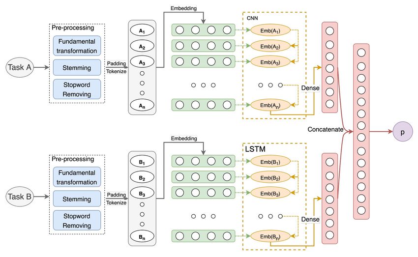
Fig. 1: The architecture of our Siamese model: a CNN layer with the number of
units of 256, and the Dense layer (Fully Connected layer) with the unit number of
256 using ReLU as the activation function, and the last layer using the activation
function Softmax to compute the final matching score between two input Jira
issues.
Table 1: Preprocessing results
Datasets Original Text Proccessed Text
< p > RPM install runs as user flume
, but a file such as/var/log/messages
rpm install run user flume file var
is default perms 600 on centos/redhat.
log message default perm centos
< /p > < p >Ideally we don’t want to run
redhat ideally want run flume
flume node as root.< /p >Flume node’s
node root flume node tail source
tail source does not report error or go
FLUME report error go error state user
into error state to user attempts to tail
attempt tail file permission read
a file it doesn’t have permissions to
flume node tail source report error
read. Flume node’s tail source does
go error state user attempt tail file
not report error or go into error state
permission read
to user attemptsto tail a file it doesn’t
have permissions to read.
< /p >Rather than writing docs AT
moodle DOT org, it would be nice to rather writing doc moodle dot
have mail to links.< /p >Add email would nice mail to link add email
MDLSITE
obfuscation to Moodle Docs Add obfuscation moodle doc add email
email obfuscation to Moodle Docs obfuscation moodle doc
Fix.
issue, such as, e.g., ”What type of this issue is?”, ”How does it affect the product
and other functions?” and ”Why does it occur?” As a result, we decide to use these
three attributes to construct a suitable recommendation model for the problem.
Moreover, to enhance the performance of those features, we also tried to extract
time features included ”Created Date” and ”Updated Date”. If they are considered
independently, these values seem to be similar in a large group of issues. Hence, we
combine them to two features called ”Cre-cre” and ”Cre-up”. They are following
an assumption that if two issues are created near each other created day, or one10 Quynh Nguyen et al.
issue is created near the day one other issue is updated, they tend to have links
between each other.
We use the Pandas library to convert all time features from string to DateTime
type for this feature. We then get the absolute value of the subtraction between two
created dates or between the created date and the updated date, as represented
above with each pair of issues.
Assume that X is an issue that we need to recommend a list of relevant matters
that link with it. Y is the issue that we aim to check if it likely has a link with X
or not. In the feature engineering step, we add two features: the gap between the
created dates of both X and Y and the gap between the created date of X and the
updated date of Y (in short, we named it CC and CU , respectively).
4.2 Model Training
This section aims to present two proposed approaches to the main problem. First,
as the primary problem can be formulated as a classification problem, we want to
estimate the matching score between the current task created and other previous
ones to choose the top K relevant items for the output results of the TaDeR
system. To construct an appropriate recommendation model from each training
dataset, we can split all Jira observations into two groups. One group contains
all existent pairs of Jira issues that link with each other (Jira users created these
links during the related project). Another group has all remaining couples of Jira
issues having no connection with others, namely “lonely issues”. We can create
initial datasets for training and testing the expected recommendation model by
this approach. We aim to build a binary classification model for estimating the
probability of having a connection between two given Jira observations using these
two groups. We label each pair as “1” if the two issues have a link between them,
and “0” if they are not relevant.
However, we need to assume that we can only utilize available attributes when
creating the current Jira issue. In the modeling process, we consider two differ-
ent directions. In this first direction, we compute TF-IDF features for all text
attributes in this first direction and combine them for the final feature vector for a
given Jira issue. We estimate their cosine similarity distance based on the feature
vectors extracted from two given Jira issues. However, the result is not so well
even when we tried to replace cosine similarity with euclidean distance, manhat-
tan distance, and Chebyshev distance. In the second approach, we construct a
Siamese neural network, where we use GloVe as our embedding and CNN layer to
compute the deep-learning features from each Jira issue’s input data. After that,
we calculate the similarity between two feature vectors computed by one Dense
layer for getting the matching score of these two issues. We later use embedding
methods with FastText and replaced CNN with GRU and LSTM.
For returning the list of recommended items, we calculate the matching scores
between the chosen Jira issues and all other previous ones and determine the list
of top K relevant items. In what follows, we will briefly describe our proposed
models.TaDeR: A New Task Dependency Recommendation 11
4.2.1 Traditional Methods
In this work, we compare many methods (from traditional to deep learning) to get
our proposed technique.
In the traditional approach, we first started with TF-IDF to vectorize all essen-
tial features, including the title, the description, and the summary, for a given Jira
issue. Then, after extracting the TF-IDF features from these three attributes, we
combine them into a feature vector and use this type of feature vector to estimate
the matching score of two given Jira issues using cosine similarity.
In addition, instead of cosine similarity, we use Euclidean distance, Manhattan
distance, and Chebyshev distance.
However, cosine similarity and Euclidean distance gave the best results on both
datasets.
One can find the corresponding experiment results related to this traditional
approach in Table 3, Table 4, Table 5, and Table 6.
4.2.2 Siamese Model
Siamese [2] is the model released by Yann Lecun et al., a variant of neural networks
that allows us to compare the similarities and differences in a pair of two objects.
Then, depending on the dataset provided, one can find a suitable technique to
compute each object’s feature vector via a shared neural network and estimate
the final matching score at the end.
The Siamese architecture used in Jira is built, as shown in Figure 1. For two
input Jira issues, we apply the necessary data processing step for each, do the
padding tokenize step, and then feed them through an embedding layer to trans-
form words into the same higher-dimensional feature space where all terms are
more closely related. We employ a CNN layer to control how much of the previous
state is retained and how many parts of the new state are the same as the primor-
dial state. After this step, we can obtain two feature vectors for two initial Jira
issues. Using a Dense layer with the Softmax activation function, the model can
output the probability of linking these two input issues. Finally, we use the MSE
as a loss function to update weights by backpropagation in the training process.
After trying combinations of CNN, GRU, LSTM with different embedding
methods included FastText and GloVe, and we found out that GloVe with CNN
brings the best results.
There are many reasons for this:
– CNN is able to extract well both local and position-invariant features. Our
dataset, however including mostly free-text and discrete information technol-
ogy major words as we can see in 1 so LSTM and GRU is not worked as well
as CNN.
– Similar to the difference between Glove and Fasttext, Glove focus more on
global statistics hence Glove’s word vectors are more discrete in the space
which lead to a better result.12 Quynh Nguyen et al.
5 Data Collection and Evaluation
Nowadays, Jira has become a proprietary issue-tracking product developed by
Atlassian, a day-to-day bug tracking and agile management dashboard of many
popular products and projects of Atlassian and other technology teams. It contains
several essential pieces of information that are adequate to explore, such as title,
description, a summary of an observation (each observation here is a task, a story,
or a project), and their linkage information.
To investigate the task dependency recommendation problem, we find available
public projects with over 3000 observations with at least 100 linkages among Jira
observations. There are two well-known data sources, including Apache9 and Moo-
dle10 . Both Apache’s teams and Moodle’s teams usually use Jira as their primary
project management platforms.
In experiments, we choose two large datasets for comparing the performance of
different methods: one Moodle project (MDLSITE11 ) and Apache project FLUME12 ).
Then, we did experiments with 28 combinations of features on FLUME since it
has fewer issues than MDLSITE. Hence the experiments will run faster. After get-
ting the best combination of features, we test different models on FLUME and
MDLSITE to find which model has the best performance.
5.1 Data Collection
The Apache software foundation (or denoted as Apache13 ) has multiple projects/products
using Jira as their primary project management dashboard. Similarly, Moodle also
has various projects/products using Jira, such as Moodle App (MOBILE), Moo-
dle QA (MDLQA), and Moodle Community Sites (MDLSITE). These are public
projects for issue tracking, and one can access these projects by their public APIs
to quickly collect or search relevant Jira observations.
Among the datasets, each Jira task collected has 32 attributes. We list these
attributes and the corresponding description at Table 17, Table 18, and Table ??.
5.2 Datasets
This section briefly describes datasets, including MDLSITE and FLUME. In ex-
periments, all data sets are split into two mutually exclusive groups: one training
set and one testing set with a ratio of 3:1. Instead of randomly dividing them,
we choose a date as a splitting point, which means all observations created before
this splitting point are training set. Other tasks made after this date belong to the
testing set. This division can help us mimic a practical application of the TaDeR
system when we utilize historical data for recommending the relevant tasks for one
Jira observation created.
9 https://projects.apache.org/projects.html
10 https://tracker.moodle.org/projects
11 (Moodle Community Sites) https://tracker.moodle.org/
12 https://flume.apache.org/
13 https://www.apache.org/TaDeR: A New Task Dependency Recommendation 13
Specifically, we can construct six corresponding datasets for datasets collected,
including three training sets and three testing sets as follows. For the MDLSITE
dataset, we choose the splitting point as the 4100th day, which means all observa-
tions created in the first 4100 days belong to the training set, and the remaining
ones are in the testing dataset. Also, we select the splitting point for the FLUME
dataset as the 1577th day.
Table 2: The details of datasets chosen FLUME and MDLSITE
FLUME MDLSITE
Issues 3373 5910
# Links 1664 4566
# Training Size 2502 4389
# Available Links (Training Dataset) 1266 3084
# Testing Size 871 1521
# Available Links (Testing Dataset) 398 1482
Ordinarily, the contents in the Summary column are replicates of the Title
column. For this reason, when we analyze these datasets, we discover that they
have pretty similar contents, and the histograms of the number of words look a
bit close.
5.3 Performance Metrics
We measure each method’s performance using the following standard metrics in
the recommendation system: Accuracy@K, Recall@K, and MRR@K.
5.3.1 Accuracy@K
For a given list of K recommended items, the metric Accuracy@K can be computed
as follows:
T P @K + T N @K
Accuracy@K =
T P @K + T N @K + F P @K + F N @K
In the top K recommended results, TP@K is the number of actual relevant pairs
predicted to be related, TN@K is the number of pairs that are irrelevant and
predicted to be irrelevant. FP@K is the number of pairs that are irrelevant but
predicted to be relevant, and FN@k is the number of pairs that are relevant but
predicted to be irrelevant.
5.3.2 Recall@K
Recall@K is one of the essential metrics that can be determined as:
T P @K
Recall@K =
T P @K + F N @K14 Quynh Nguyen et al.
5.3.3 Mean Reciprocal Rank@K
The formula of Mean Reciprocal Rank@K (MRR@K) can be given as follows
|K|
1 X 1
M RR = ,
|K| i=1 ranki
where ranki denotes the rank of the first relevant result and K is the top relevant
issues.
6 Experiments
There are three fascinating questions we aim to investigate related to the task de-
pendency recommendation system in our experiments. First, what types of existing
attributes from a new Jira task created are vital to the corresponding model? In
practice, most possible tasks likely related to a given one are usually created dur-
ing the last few months. Consequently, what is the impact of using time filtering
on the final recommendation results of the TaDeR system? Finally, how much does
using deep learning features and the Siamese architecture help increase a TaDeR
system’s performance in chosen datasets?
All experiments are operated on a computer with Intel(R)-Core(TM)-i7 2
CPUs running at 2.4GHz, 128GB of RAM, and an Nvidia GeForce RTX-2080Ti
GPU. We present our experimental design and the corresponding results concern-
ing these research questions in what follows.
6.1 Experimental Design
As mentioned in the previous section, we first use dataset FLUME to find the
best features and then compare all proposed methods on FLUME and MDLSITE.
MDLSITE dataset has too many issues that took a long time to train for each
model, so we only use FLUME for this experiment. We use five valuable attributes
from the input data of a new Jira task created: Title (T), Description (D), Sum-
mary (S), Created Date, and Updated Date. For two specific Jira issues, we extract
the following features: Title (T), Description (D), Summary (S), the gap between
their created dates (CC or C2), the absolute difference between the created date
of the current issue chosen and the updated date of another one, namely (CU).
In these experiments, we use four different numbers of top features: K =
1, 2, 3, 5. For each value of K, we measure the performance of the corresponding
type of features computed and the selected model using Accuracy@K, Recall@K
and MRR@K. We also do extensive experiments by considering 28 combinations
of five features computed (T, D, S, C2, and CU) to understand the impact of
each type of feature combination of the model. These 28 features are as follows:
T (Title), D (Description), S (Summary), TD (Title + Description), TS (Title
+ Summary), TDS (Title + Description + Summary), DS (Description + Sum-
mary), TC2 (Title +C2), DC2 (Description + C2), SC2 (Summary + C2), TDC2
(Title + Description + C2), TSC2 (Title + Summary + C2), TDSC2 (Title + De-
scription + Summary + C2), DSC2 (Description + Summary + C2), TCU (TitleTaDeR: A New Task Dependency Recommendation 15
+ CU), DCU (Description + CU), SCU (Summary + CU), TDCU (Title + De-
scription + CU), TSCU (Title + Summary + CU), TDSCU (Title + Description
+ Summary + CU), DSCU (Description + Summary + CU), TC2CU (Title +
C2 + CU), DC2CU (Description + C2 + CU), SC2CU (Summary + C2 + CU),
TDC2CU (Title + Description + C2 + CU), TSC2CU (Title + Summary + C2
+ CU), TDSC2CU (Title + Description + Summary+ C2 + CU), and DSC2CU
(Description + Summary+ C2 + CU).
After finding out the best features, we tested these features with several com-
binations of two embedding methods (GloVe and FastText) and 3 model types
(LSTM, GRU, and CNN).
Besides, we consider seven scenarios of applying the “time filter” to get the
recommended items list in the post-processing step for a TaDeR system. In our
work, we select the following “time filter”: one month, two months, three months,
and no time filter.
For the traditional approach, we compute the corresponding performance of
the proposed models (TF-IDF for feature extraction with several techniques for
estimating matching scores) for datasets.
6.2 Hyperparameter Tuning
After experiments, we began to tune our best model - GloVe Embedding and
CNN model to get the best result. We apply the hyperparameter tuning process
to find our proposed Siamese architecture’s best configuration for the TaDeR sys-
tem. Those hyperparameters of all hidden layers (LSTM and Dense Layer) are
the number of units and the action functions. Using two experimental datasets
provided, we do the following hyperparameter tuning process:
– The number of units can be finetuned as follows. All unit numbers of an LSTM
layer and a fully connected (FC) layer start from 50 units at the beginning.
Sequentially, we can increase each unit number by 50 units every step, and it
will be stopped either the evaluation metrics stop growing or the loss value is
not convergent.
– We have tried some typical activation functions (ReLU, LeakyReLU, and Sig-
moid) for the Dense layer, and the activation function ReLU shows that it is
the most sufficient in this problem.
7 Discussions
As mentioned in Section 6, we aimed to answer our first question about the at-
tributes that are the best for our corresponding model. Since there are many
issues in the MDLSITE dataset, we decided to perform the first 28 experiments
on FLUME instead. We chose a combination of features in each experiment and
applied them on GloVe and CNN model with the default 2-month timing filter.
We have seven combinations with three textual features (Title – T, Description –
D, Summary – S): T, D, S, DT, DS, DTS, and TS. Table 7 and Table 8 showed
that DTS brings the best result among them with Accuracy@1 and MRR@1 reach
0.2026, Recall@1 obtains 0.1698. Using only title (T) and TS (title and summary)
bring the worst results, with Accuracy@1 only 0.0529 and 0.0441. To exploit the16 Quynh Nguyen et al.
impact of our observation (issues created near each other usually have links be-
tween them), we added the feature CC, as mentioned in Section 5. After adding
this feature, DTS + CC is the best result and is higher than DTS 0.01 in all
Accuracy, MRR, and Recall.
The last updated time seemed to affect our problem, so we added the CU
feature. DTS + CC + CU now is the best result in these experiments where MRR
reaches 0.2291 and Recall can be obtained as 0.1956. This result is also higher than
0.01 compared with DTS + CC and 0.02 compared with DTS. After knowing the
best attributes for our corresponding model, we tried various embeddings and
structures to have the best model.
In Table 9 and Table 10, when we tried 6 different models: GloVe + LSTM,
GloVe + GRU, GloVe + CNN, FastText + LSTM, FastText + GRU, and Fast-
Text + CNN with no timing filter on both dataset: FLUME and MDLSITE. In
these experiments, these results are quite different between these datasets. With
FLUME, FastText + LSTM reaches the best result but in MDLSITE, FastText
+ GRU is the best model. However, these results are lower than cosine similarity
and Euclidean distance in traditional approaches.
Adding a timing filter can speed up the computational time while still keeping
the same as or better performance than searching in all historical Jira tasks of
a given project. From Table 11 to Table 16, we tried a 1-month timing filter, 2-
month timing filter and 3-month timing filter. With a 1-month timing filter, GloVe
+ CNN and FastText + LSTM bring the best results. Compared to FLUME,
GloVe + CNN are the only models with Accuracy@1, MRR@1 higher than cosine
similarity, and Euclidean distance in the traditional approach. Hence, we decided
to propose this model.
When analyzing the top 3 and top 5 results, Accuracy, MRR, and Recall were
reduced when the timing filter increased from one month to three months, the
same with the MDLSITE dataset. From this observation, a 1-month timing filter
is the best timing filter for this problem.
We conclude from all analysis above that GloVe + CNN and a 1-month timing
filter will be a proper model to solve our problem. This model reached 0.2335 in
accuracy@1 and MRR@1 in the FLUME dataset. With the MDLSITE dataset,
this model reaches 0.1258 in accuracy@1 and MRR@1. These results are higher
than our best in the traditional approach, about 0.001 in accuracy@1 and MRR@1
and 0.2 in Recall@1 for MDLSITE. With FLUME, these results are higher than
0.001 in accuracy@1 and MRR@1 and 0.5 in Recall@1. With top 3 and top 5 on
FLUME, accuracy@3 and Recall@3 are lower than the traditional approach, but
MRR@3 is higher than 0.006, and MRR@5 and Recall@5 are higher 0.01 compared
to the conventional methods.
8 Conclusion and Future Works
We have presented an extensive study for building a task dependency recommen-
dation system in project management platforms. We have compared two differ-
ent methods by considering a traditional one (using TF-IDF features and many
distance metrics for estimating the matching score between the current task cre-
ated and a specific task) and proposing an efficient Siamese network (using oneTaDeR: A New Task Dependency Recommendation 17
Table 3: Traditional methods on dataset FLUME - Top 1 and Top 2
Top 1 Top 2
Distance metrics
Accuracy MRR Recall Accuracy MRR Recall
Chebysev Distance 0.1189 0.1189 0.0737 0.1189 0.1189 0.0769
Cosine Similarity 0.2203 0.2203 0.1589 0.2203 0.2203 0.1589
Euclidean Distance 0.2203 0.2203 0.1589 0.2203 0.2203 0.1589
Manhattan Distance 0.1366 0.1366 0.0903 0.1366 0.1366 0.0903
Table 4: Traditional methods on dataset FLUME - Top 3 and Top 5
Top 3 Top 5
Distance metrics
Accuracy MRR Recall Accuracy MRR Recall
Chebysev Distance 0.1322 0.1233 0.1004 0.1454 0.1264 0.1153
Cosine Similarity 0.2863 0.2423 0.2392 0.3172 0.2485 0.2584
Euclidean Distance 0.2863 0.2423 0.2392 0.3172 0.2485 0.2584
Manhattan Distance 0.1982 0.1571 0.1629 0.2291 0.1633 0.1903
Table 5: Traditional methods on dataset MDLSITE - Top 1 and Top 2
Top 1 Top 2
Distance metrics
Accuracy MRR Recall Accuracy MRR Recall
Chebysev Distance 0.0679 0.0679 0.0454 0.0767 0.0723 0.0521
Cosine Similarity 0.1245 0.1245 0.0905 0.1245 0.1245 0.0905
Euclidean Distance 0.1245 0.1245 0.0905 0.1245 0.1245 0.0905
Manhattan Distance 0.0893 0.0893 0.0632 0.0893 0.0893 0.0632
Table 6: Traditional methods on dataset MDLSITE - Top 3 and Top 5
Top 3 Top 5
Distance metrics
Accuracy MRR Recall Accuracy MRR Recall
Chebysev Distance 0.0855 0.0753 0.0595 0.0956 0.0773 0.0672
Cosine Similarity 0.1434 0.1308 0.1111 0.1547 0.1331 0.1222
Euclidean Distance 0.1434 0.1308 0.1111 0.1547 0.1331 0.1222
Manhattan Distance 0.1019 0.0935 0.0766 0.1082 0.0948 0.0799
GloVe Embedding, one CNN layer, and a Dense layer) for building the correspond-
ing recommendation. We compare these methods using datasets (MDLSITE and
FLUME) and the performance metrics Recall@K, Accuracy@K, and MRR@K.
The experimental results show that the proposed method can outperform the tra-
ditional one in all datasets (increasing about 0.01 in Accuracy and MRR and 0.05
in Recall). Also, using the time filter can efficiently help enhance the performance
of the TaDeR system.
There are still some limitations related to the TaDeR system. The current
problem only focuses on recommending the top relevant tasks with a given Jira18 Quynh Nguyen et al.
Table 7: Best features experiment on FLUME - Top 1 and Top 2 (using the two-
month timing filter)
Top 1 Top 2
Features
Accuracy MRR Recall Accuracy MRR Recall
T 0.0529 0.0529 0.0395 0.0705 0.0771 0.0577
D 0.1057 0.1057 0.0879 0.1189 0.1454 0.0982
S 0.1145 0.1145 0.0905 0.1542 0.1674 0.1278
DT 0.0749 0.0749 0.0624 0.1013 0.1145 0.0777
DS 0.0749 0.0749 0.0628 0.0793 0.1079 0.0662
DTS 0.2026 0.2026 0.1698 0.2203 0.2952 0.1824
TS 0.0441 0.0441 0.0279 0.0749 0.0727 0.0558
T + CC 0.0749 0.0749 0.0598 0.1233 0.1189 0.0994
D + CC 0.1938 0.1938 0.1637 0.2115 0.2885 0.1809
S + CC 0.0485 0.0485 0.0292 0.0837 0.0771 0.0615
DT + CC 0.0969 0.0969 0.0770 0.1145 0.1366 0.0887
DS + CC 0.0881 0.0881 0.0624 0.1101 0.1322 0.0862
DTS + CC 0.2115 0.2115 0.1787 0.2247 0.3062 0.1876
TS + CC 0.0485 0.0485 0.0406 0.0925 0.0859 0.0718
T + CU 0.0705 0.0705 0.0527 0.1057 0.1167 0.0789
D + CU 0.1718 0.1718 0.1559 0.2026 0.2555 0.1787
S + CU 0.0573 0.0573 0.0492 0.1057 0.0947 0.0807
DT + CU 0.0705 0.0705 0.0507 0.0881 0.1057 0.0665
DS + CU 0.0749 0.0749 0.0606 0.0881 0.1101 0.0679
DTS + CU 0.1762 0.1762 0.1545 0.2026 0.2709 0.1754
TS + CU 0.1762 0.1762 0.1534 0.2291 0.2467 0.2030
T + CC + CU 0.0617 0.0617 0.0499 0.0793 0.0903 0.0638
D + CC + CU 0.1806 0.1806 0.1545 0.2115 0.2797 0.1838
S + CC + CU 0.0793 0.0793 0.0564 0.1101 0.1057 0.0795
DT + CC + CU 0.0793 0.0793 0.0613 0.1013 0.1189 0.0792
DS + CC + CU 0.0705 0.0705 0.0562 0.0749 0.1013 0.0614
DTS + CC + CU 0.2291 0.2291 0.1956 0.2467 0.3348 0.2095
TS + CC + CU 0.0705 0.0705 0.0437 0.0925 0.1057 0.0645
observation created. It is fascinating if the TaDeR system can suggest top-related
tasks and classify users’ corresponding types of links. We aim to apply other em-
bedding methods and extend our experiments to other challenging datasets in
future work.
References
1. Bojanowski P, Grave E, Joulin A, Mikolov T (2016) Enriching word vectors
with subword information. arXiv preprint arXiv:160704606TaDeR: A New Task Dependency Recommendation 19
Table 8: Best features experiment on FLUME - Top 3 and Top 5 (using the two-
month timing filter)
Top 3 Top 5
Features
Accuracy MRR Recall Accuracy MRR Recall
T 0.1233 0.1035 0.0952 0.1630 0.1194 0.1241
D 0.1454 0.1630 0.1177 0.1674 0.1883 0.1433
S 0.2159 0.1982 0.1858 0.2996 0.2313 0.2618
DT 0.1189 0.1322 0.0970 0.2203 0.1742 0.1819
DS 0.1057 0.1211 0.0841 0.1806 0.1511 0.1549
DTS 0.2511 0.3172 0.2067 0.2731 0.3423 0.2297
TS 0.1101 0.0918 0.0777 0.1498 0.1123 0.1059
T + CC 0.1718 0.1439 0.1446 0.2731 0.1785 0.2465
D + CC 0.2247 0.3018 0.1934 0.2511 0.3262 0.2224
S + CC 0.1322 0.0977 0.1044 0.2247 0.1338 0.1798
DT + CC 0.1233 0.1468 0.0943 0.1278 0.1609 0.0985
DS + CC 0.1586 0.1571 0.1298 0.2203 0.1838 0.1899
DTS + CC 0.2467 0.3282 0.2032 0.2907 0.3498 0.2455
TS + CC 0.1057 0.0977 0.0835 0.1410 0.1153 0.1073
T + CU 0.1322 0.1329 0.0991 0.1806 0.1521 0.1456
D + CU 0.2379 0.2878 0.2054 0.2643 0.3019 0.2297
S + CU 0.1586 0.1182 0.1233 0.2731 0.1640 0.2234
DT + CU 0.1278 0.1248 0.0995 0.2247 0.1662 0.1839
DS + CU 0.1145 0.1248 0.0866 0.1586 0.1455 0.1243
DTS + CU 0.2291 0.2915 0.1985 0.2467 0.3084 0.2105
TS + CU 0.2555 0.2805 0.2213 0.2687 0.3045 0.2311
T + CC + CU 0.1233 0.1094 0.0935 0.1762 0.1321 0.1385
D + CC + CU 0.2203 0.2930 0.1929 0.2555 0.3145 0.2319
S + CC + CU 0.1454 0.1351 0.1089 0.1762 0.1547 0.1408
DT + CC + CU 0.1278 0.1395 0.1022 0.1938 0.1624 0.1664
DS + CC + CU 0.0925 0.1116 0.0734 0.1189 0.1255 0.0891
DTS + CC + CU 0.2555 0.3495 0.2201 0.2819 0.3728 0.2455
TS + CC + CU 0.1410 0.1322 0.1118 0.2070 0.1608 0.1712
2. Bromley J, Guyon I, LeCun Y, Säckinger E, Shah R (1993) Signature verifica-
tion using a ”siamese” time delay neural network. In: Proceedings of the 6th
International Conference on Neural Information Processing Systems, Morgan
Kaufmann Publishers Inc., San Francisco, CA, USA, NIPS’93, p 737–744
3. Cao HK, Cao HK, Nguyen BT (2020) Delafo: An efficient portfolio optimiza-
tion using deep neural networks. In: Lauw HW, Wong RCW, Ntoulas A, Lim
EP, Ng SK, Pan SJ (eds) Advances in Knowledge Discovery and Data Mining,
Springer International Publishing, Cham, pp 623–635
4. Choetkiertikul M, Dam HK, Tran T, Ghose A (2015) Predicting delays in
software projects using networked classification (t). In: 2015 30th IEEE/ACM20 Quynh Nguyen et al.
Table 9: Experiments with no time filter - Top 1 and Top 2
Top 1 Top 2
Model
Accuracy MRR Recall Accuracy MRR Recall
FLUME
GloVe + LSTM 0.0881 0.0881 0.0630 0.2159 0.1520 0.1774
GloVe + GRU 0.0441 0.0441 0.0183 0.1542 0.0991 0.1100
GloVe + CNN 0.0000 0.0000 0.0000 0.0000 0.0000 0.0000
FastText + LSTM 0.1674 0.1674 0.1589 0.1894 0.1784 0.1750
FastText + GRU 0.0881 0.0881 0.0837 0.1057 0.0969 0.0977
FastText + CNN 0.1233 0.1233 0.1149 0.1850 0.1542 0.1685
MDLSITE
GloVe + LSTM 0.0252 0.0252 0.0160 0.0377 0.0314 0.0260
GloVe + GRU 0.0000 0.0000 0.0000 0.0000 0.0000 0.0000
GloVe + CNN 0.0000 0.0000 0.0000 0.0000 0.0000 0.0000
FastText + LSTM 0.0013 0.0013 0.0001 0.2063 0.1038 0.1991
FastText + GRU 0.0956 0.0956 0.0848 0.2465 0.1711 0.2351
FastText + CNN 0.0000 0.0000 0.0000 0.1447 0.0723 0.1432
Table 10: Experiments with no time filter - Top 3 and Top 5
Top 3 Top 5
Model
Accuracy MRR Recall Accuracy MRR Recall
FLUME
GloVe + LSTM 0.2467 0.1623 0.2005 0.3392 0.1827 0.2856
GloVe + GRU 0.2291 0.1241 0.1845 0.3040 0.1408 0.2515
GloVe + CNN 0.0000 0.0000 0.0000 0.0705 0.0170 0.0683
FastText + LSTM 0.2467 0.1975 0.2326 0.3084 0.2123 0.2916
FastText + GRU 0.1938 0.1263 0.1721 0.2379 0.1364 0.2101
FastText + CNN 0.1938 0.1571 0.1706 0.2159 0.1624 0.1909
MDLSITE
GloVe + LSTM 0.0503 0.0356 0.0355 0.0755 0.0416 0.0570
GloVe + GRU 0.0239 0.0080 0.0153 0.0478 0.0132 0.0337
GloVe + CNN 0.0252 0.0084 0.0252 0.0830 0.0206 0.0774
FastText + LSTM 0.3321 0.1457 0.3218 0.4453 0.1708 0.4311
FastText + GRU 0.3799 0.2155 0.3660 0.4969 0.2427 0.4774
FastText + CNN 0.2818 0.1180 0.2779 0.4604 0.1612 0.4547
International Conference on Automated Software Engineering (ASE), pp 353–
364, DOI 10.1109/ASE.2015.55
5. Chung J, Gülçehre Ç, Cho K, Bengio Y (2014) Empirical evaluation of gated
recurrent neural networks on sequence modeling. CoRR abs/1412.3555, URL
http://arxiv.org/abs/1412.3555, 1412.3555TaDeR: A New Task Dependency Recommendation 21
Table 11: Experiments with time filter 1 month - Top 1 and Top 2
Top 1 Top 2
Model
Accuracy MRR Recall Accuracy MRR Recall
FLUME
GloVe + LSTM 0.0837 0.0837 0.0586 0.2115 0.1476 0.1730
GloVe + GRU 0.0396 0.0396 0.0139 0.1498 0.0947 0.1056
GloVe + CNN 0.2335 0.2335 0.2011 0.2511 0.2423 0.2216
FastText + LSTM 0.2026 0.2026 0.1882 0.2335 0.2181 0.2144
FastText + GRU 0.1410 0.1410 0.1210 0.1674 0.1542 0.1411
FastText + CNN 0.2026 0.2026 0.1627 0.2070 0.2048 0.1699
MDLSITE
GloVe + LSTM 0.0252 0.0252 0.0160 0.0377 0.0314 0.0260
GloVe + GRU 0.0314 0.0314 0.0211 0.0415 0.0365 0.0290
GloVe + CNN 0.1258 0.1258 0.1141 0.2541 0.1899 0.2401
FastText + LSTM 0.2302 0.2302 0.2243 0.3610 0.2956 0.3537
FastText + GRU 0.1308 0.1308 0.1216 0.2881 0.2094 0.2762
FastText + CNN 0.1836 0.1836 0.1779 0.3233 0.2535 0.3136
Table 12: Experiments with time filter 1 month - Top 3 and Top 5
Top 3 Top 5
Model
Accuracy MRR Recall Accuracy MRR Recall
FLUME
GloVe + LSTM 0.2379 0.1564 0.1917 0.3304 0.1769 0.2767
GloVe + GRU 0.2203 0.1182 0.1757 0.2952 0.1349 0.2426
GloVe + CNN 0.2687 0.2482 0.2377 0.3040 0.2563 0.2651
FastText + LSTM 0.2996 0.2401 0.2786 0.3524 0.2520 0.3225
FastText + GRU 0.2555 0.1836 0.2225 0.3040 0.1943 0.2698
FastText + CNN 0.2247 0.2107 0.1890 0.2907 0.2253 0.2535
MDLSITE
GloVe + LSTM 0.0503 0.0356 0.0355 0.0767 0.0418 0.0576
GloVe + GRU 0.0516 0.0398 0.0371 0.0780 0.0461 0.0581
GloVe + CNN 0.3975 0.2377 0.3765 0.5270 0.2689 0.5018
FastText + LSTM 0.4277 0.3178 0.4157 0.5220 0.3386 0.5053
FastText + GRU 0.3925 0.2442 0.3792 0.5308 0.2753 0.5103
FastText + CNN 0.4730 0.3034 0.4594 0.5648 0.3230 0.5418
6. Duchi J, Hazan E, Singer Y (2011) Adaptive subgradient methods for online
learning and stochastic optimization. Journal of Machine Learning Research
12(Jul):2121–2159
7. Hochreiter S (1998) The vanishing gradient problem during learning recur-
rent neural nets and problem solutions. International Journal of Uncertainty,
Fuzziness and Knowledge-Based Systems 6:107–116, DOI 10.1142/S021848822 Quynh Nguyen et al.
Table 13: Experiments with time filter 2 months - Top 1 and Top 2
Top 1 Top 2
Model
Accuracy MRR Recall Accuracy MRR Recall
FLUME
GloVe + LSTM 0.0837 0.0837 0.0586 0.2115 0.1476 0.1730
GloVe + GRU 0.0396 0.0396 0.0139 0.1498 0.0947 0.1056
GloVe + CNN 0.2291 0.2291 0.1956 0.2467 0.2379 0.2095
FastText + LSTM 0.1718 0.1718 0.1633 0.1982 0.1850 0.1846
FastText + GRU 0.1013 0.1013 0.0914 0.1366 0.1189 0.1159
FastText + CNN 0.1762 0.1762 0.1523 0.2026 0.1894 0.1636
MDLSITE
GloVe + LSTM 0.0252 0.0252 0.0160 0.0377 0.0314 0.0260
GloVe + GRU 0.0289 0.0289 0.0185 0.0390 0.0340 0.0265
GloVe + CNN 0.1346 0.1346 0.1165 0.2667 0.2006 0.2461
FastText + LSTM 0.2289 0.2289 0.2212 0.3560 0.2925 0.3477
FastText + GRU 0.0981 0.0981 0.0890 0.2792 0.1887 0.2657
FastText + CNN 0.1811 0.1811 0.1757 0.3157 0.2484 0.3064
Table 14: Experiments with time filter 2 months - Top 3 and Top 5
Top 3 Top 5
Model
Accuracy MRR Recall Accuracy MRR Recall
FLUME
GloVe + LSTM 0.2379 0.1564 0.1917 0.3304 0.1769 0.2767
GloVe + GRU 0.2203 0.1182 0.1757 0.2952 0.1349 0.2426
GloVe + CNN 0.2555 0.2408 0.2201 0.2819 0.2470 0.2455
FastText + LSTM 0.2687 0.2085 0.2553 0.3128 0.2189 0.2910
FastText + GRU 0.2115 0.1439 0.1834 0.2467 0.1516 0.2164
FastText + CNN 0.2247 0.1968 0.1860 0.2555 0.2034 0.2190
MDLSITE
GloVe + LSTM 0.0503 0.0356 0.0355 0.0755 0.0416 0.0570
GloVe + GRU 0.0516 0.0382 0.0371 0.0780 0.0444 0.0581
GloVe + CNN 0.3786 0.2379 0.3553 0.5182 0.2701 0.4929
FastText + LSTM 0.4226 0.3147 0.4105 0.5145 0.3350 0.4981
FastText + GRU 0.3824 0.2231 0.3662 0.5182 0.2546 0.4957
FastText + CNN 0.4642 0.2979 0.4499 0.5258 0.3117 0.5055
598000094
8. Indolia S, Goswami AK, Mishra S, Asopa P (2018) Conceptual understanding
of convolutional neural network- a deep learning approach. Procedia Computer
Science 132:679–688, DOI https://doi.org/10.1016/j.procs.2018.05.069, URL
https://www.sciencedirect.com/science/article/pii/S187705091830801
9, international Conference on Computational Intelligence and Data ScienceTaDeR: A New Task Dependency Recommendation 23
Table 15: Experiments with time filter 3 months - Top 1 and Top 2
Top 1 Top 2
Model
Accuracy MRR Recall Accuracy MRR Recall
FLUME
GloVe + LSTM 0.0837 0.0837 0.0586 0.2115 0.1476 0.1730
GloVe + GRU 0.0396 0.0396 0.0139 0.1498 0.0947 0.1056
GloVe + CNN 0.2247 0.2247 0.1986 0.2423 0.2335 0.2092
FastText + LSTM 0.1674 0.1674 0.1589 0.1982 0.1828 0.1846
FastText + GRU 0.1013 0.1013 0.0914 0.1322 0.1167 0.1153
FastText + CNN 0.1718 0.1718 0.1512 0.1894 0.1806 0.1592
MDLSITE
GloVe + LSTM 0.0252 0.0252 0.0160 0.0377 0.0314 0.0260
GloVe + GRU 0.0264 0.0264 0.0158 0.0377 0.0321 0.0250
GloVe + CNN 0.1258 0.1258 0.1049 0.2679 0.1969 0.2487
FastText + LSTM 0.2277 0.2277 0.2199 0.3346 0.2811 0.3249
FastText + GRU 0.0931 0.0931 0.0846 0.2465 0.1698 0.2340
FastText + CNN 0.1774 0.1774 0.1734 0.3157 0.2465 0.3060
Table 16: Experiments with time filter 3 months - Top 3 and Top 5
Top 3 Top 5
Model
Accuracy MRR Recall Accuracy MRR Recall
FLUME
GloVe + LSTM 0.2379 0.1564 0.1917 0.3304 0.1769 0.2767
GloVe + GRU 0.2203 0.1182 0.1757 0.2952 0.1349 0.2426
GloVe + CNN 0.2467 0.2349 0.2127 0.2775 0.2420 0.2396
FastText + LSTM 0.2643 0.2048 0.2509 0.3084 0.2150 0.2920
FastText + GRU 0.2115 0.1432 0.1826 0.2379 0.1491 0.2101
FastText + CNN 0.2115 0.1880 0.1787 0.2423 0.1946 0.2061
MDLSITE
GloVe + LSTM 0.0503 0.0356 0.0355 0.0755 0.0416 0.0570
GloVe + GRU 0.0528 0.0371 0.0375 0.0767 0.0426 0.0579
GloVe + CNN 0.3560 0.2262 0.3357 0.5195 0.2641 0.4943
FastText + LSTM 0.4063 0.3050 0.3935 0.5094 0.3284 0.4945
FastText + GRU 0.3824 0.2151 0.3660 0.5157 0.2462 0.4932
FastText + CNN 0.4553 0.2931 0.4444 0.5182 0.3072 0.5000
9. Kingma DP, Ba J (2014) Adam: A method for stochastic optimization. URL
http://arxiv.org/abs/1412.6980, cite arxiv:1412.6980Comment: Published
as a conference paper at the 3rd International Conference for Learning Rep-
resentations, San Diego, 2015
10. Lam AN, Nguyen AT, Nguyen HA, Nguyen TN (2017) Bug localization with
combination of deep learning and information retrieval. In: 2017 IEEE/ACMYou can also read