RAILS: A Robust Adversarial Immune-inspired Learning System
←
→
Page content transcription
If your browser does not render page correctly, please read the page content below
RAILS: A Robust Adversarial Immune-inspired
                                                               Learning System

                                                        Ren Wang∗                     Tianqi Chen                   Stephen Lindsly
                                                   University of Michigan         University of Michigan          University of Michigan
arXiv:2107.02840v1 [cs.NE] 27 Jun 2021

                                                    Cooper Stansbury              Alnawaz Rehemtulla               Indika Rajapakse
                                                   University of Michigan         University of Michigan          University of Michigan

                                                                                      Alfred Hero
                                                                                  University of Michigan

                                                                                        Abstract

                                                     Adversarial attacks against deep neural networks (DNNs) are continuously evolv-
                                                     ing, requiring increasingly powerful defense strategies. We develop a novel ad-
                                                     versarial defense framework inspired by the adaptive immune system: the Robust
                                                     Adversarial Immune-inspired Learning System (RAILS). Initializing a population
                                                     of exemplars that is balanced across classes, RAILS starts from a uniform label
                                                     distribution that encourages diversity and debiases a potentially corrupted initial
                                                     condition. RAILS implements an evolutionary optimization process to adjust the
                                                     label distribution and achieve specificity towards ground truth. RAILS displays
                                                     a tradeoff between robustness (diversity) and accuracy (specificity), providing a
                                                     new immune-inspired perspective on adversarial learning. We empirically validate
                                                     the benefits of RAILS through several adversarial image classification experiments
                                                     on MNIST, SVHN, and CIFAR-10 datasets. For the PGD attack, RAILS is found
                                                     to improve the robustness over existing methods by ≥ 5.62%, 12.5% and 10.32%,
                                                     respectively, without appreciable loss of standard accuracy.

                                         1       Introduction
                                         The state of the art in supervised deep learning has dramatically improved over the past decade [14].
                                         Deep learning techniques have led to significant advances in applications such as: face recognition
                                         [17]; object detection [30]; and natural language processing [28]. Despite these successes, deep
                                         learning techniques are not resilient to evasion attacks on test inputs and poisoning attacks on training
                                         data [9, 25, 11]. The adversarial vulnerability of deep neural networks (DNN) have restricted their
                                         application, motivating researchers to develop effective defense methods. The focus of this paper is
                                         to develop a novel deep defense framework inspired by the mammalian immune system.
                                         Current defense methods can be broadly divided into three classes: (1) Adversarial example detection
                                         [18, 8, 10]; (2) Robust training [16, 29, 6]; and (3) Deep classifiers with natural robustness [20, 22].
                                         The first class of methods defends a DNN using simple outlier detection models for detecting
                                         adversarial examples. However, it has been shown that adversarial detection methods are not perfect
                                         and can be easily defeated [5]. Robust training aims to harden the model to deactivate attacks such as
                                         evasion attacks. Known robust training methods are often tailored to a certain level of attack strength
                                         in the context of `p -perturbation. Moreover, the trade-off between accuracy and robustness presents
                                             ∗
                                                 renwang@umich.edu; Codes are available at https://github.com/wangren09/RAILS.

                                         Preprint. Under review.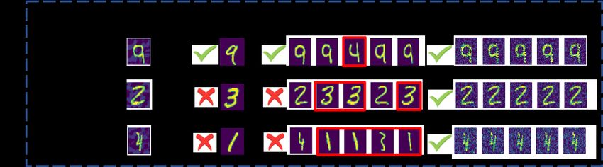
challenges [29]. Recently alternative defense strategies have been proposed that implement different
structures that are naturally resilient to evasion attacks on DNNs. Despite these advances, current
methods have difficulty providing an acceptable level of robustness to novel attacks [2].
To design an effective defense, it is natural to consider a learning strategy that emulates mechanisms
of the naturally robust biological immune system. In this paper, we propose a new framework,
Robust Adversarial Immune-inspired Learning System (RAILS), that can effectively defend deep
learning architectures against aggressive attacks. Built upon a class-wise k-Nearest Neighbor (kNN)
structure, given a test sample RAILS finds an initial small population of proximal samples, balanced
across different classes, with uniform label distribution. RAILS then promotes the specificity of the
label distribution towards the ground truth label through an evolutionary optimization. RAILS can
efficiently correct adversarial label flipping by balancing label diversity against specificity. While
RAILS can be applied to defending against many different types of attacks, in this paper we restrict
attention to evasion attacks on the input. Figure 1 (a) shows that RAILS outperforms existing methods
on various types of evasion attacks.

                           (a)                                                       (b)

Figure 1: RAILS launches the best defense against different types of attacks (left panel) using the adver-
sarial deep learning architecture shown on right panel. (a) Radar plot showing that RAILS has higher robust
accuracy than the adversarially trained CNN [16] and Deep k-Nearest Neighbor (DkNN) [20] in defending
against four types of attacks: PGD [16], Fast Gradient Sign Method (FGSM) [9], Square Attack [1], and
a (customized) kNN-attack. (b) For each test input, a special type of data - plasma data - is generated by
evolutionary optimization, that contributes to predicting the class of the input (test) sample. Another type of data
- memory data - is generated and stored to help defend against similar attacks in the future. Plasma data and
memory data are analogous to plasma B cells and memory B cells in the immune system.

Contributions. Compared to existing defense methods, we make the following contributions:
• RAILS achieves better adversarial robustness by assigning a uniform label distribution to each input
and evolving it to a distribution that is concentrated about the input’s true label class. (see Section 2
and Table 2)
• RAILS incorporates a life-long robustifying process by adding synthetic “virtual data” to the
training data. (see Section 2 and Table 3)
• RAILS evolves the distribution via mutation and cross-over mechanisms and is not restricted to `p
or any other specific type of attack. (see Section 3 and Figure 1)
• We demonstrate that RAILS improves robustness of existing methods for different types of attacks
(Figure 1). Specifically, RAILS improves robustness against PGD attack by ≥ 5.62%/12.5%/10.32%
for the MNIST, SVHN, and CIFAR-10 datasets (Table 2). Furthermore, we show that RAILS life-long
learning process provides a 2.3% robustness improvement with only 5% augmentation of the training
data (Table 3).
• RAILS is the first adversarial defense framework to be based on the biology of the adaptive immune
system. In particular: (a) RAILS computationally emulates the principal mechanisms of the immune
response (Figure 3); and (b) our computational and biological experiments demonstrate the fidelity of
the emulation - the learning patterns of RAILS and the immune system are closely aligned (Figure 6).

                                                         2
Related work. After it was established that DNNs were vulnerable to evasion attacks [25], different
types of defense mechanisms have been proposed in recent years. One intuitive idea is to eliminate
the adversarial examples through outlier detection, including training an additional discrimination
sub-network [18, 10] and using kernel density estimation [8]. The above approaches rely on the
fundamental assumption that the distributions of benign and adversarial examples are distinct, an
assumption that has been challenged in [5].
In addition to adversarial attack detection, other methods have been proposed that focus on robustify-
ing the deep architecture during the learning phase [16, 6, 29]. Though these defenses are effective
against adversarial examples with a certain level of `p attack strength, they have limited defense
power on stronger attacks, and there is often a sacrifice in overall classification accuracy. In contrast,
RAILS is developed to defend against diverse powerful attacks with less sacrifice in accuracy, and
can improve any model’s robustness, including robust models.
Another approach is to leverage different structures or classifiers on robustifying deep classifiers
[20, 22]. An example is the deep k-Nearest Neighbor (DkNN) classifier [20] that robustifies against
instance perturbations by applying kNN’s to features extracted from each layer. However, a single
kNN classifier applied on the whole dataset is easily to be fooled by strong attacks, as illustrated in
Figure 2. On the other side, RAILS incorporates a diversity to specificity defense mechanism which
can provide additional robustness to existing DNNs.
Another line of research relevant to ours is adversarial transfer learning [15, 23], which aims to
maintain robustness when there is covariate shift from training data to test data. We remark that
covariate shift is naturally handled by RAILS as it emulates the immune system which adapts to
novel mutated attacks.
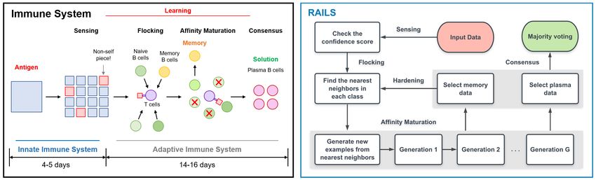
Figure 2: Representation examples showing RAILS correcting (improving) the wrong (unconfident)
predictions by CNN and kNN. kNN predict all three examples with ≤ 100% confidence of the ground truth
class, and CNN gets wrong predictions for images 2 and 4. RAILS provides correct predictions with high
confidence scores.
0
Notation and preliminaries. Given a mapping f : Rd → Rd and x1 , x2 ∈ Rd , we first define
the affinity score A(f ; x1 , x2 ) between x1 and x2 . This affinity score can be defined in many
ways, e.g, cosine similarity, inner product, or inverse `p distance, but here we use A(f ; x1 , x2 ) =
−kf (x1 ) − f (x2 )k2 , the negative Euclidean distance. In the context of DNN, f denotes the feature
mapping from input to feature representation, and A measures the similarity between two inputs.
Higher affinity score indicates higher similarity.
2 RAILS: overview
In this section, we give an overview of RAILS, and provide a comparison to the natural immune
system.
The architecture of RAILS is illustrated in the right panel of Figure 1. For each selected hidden layer
l, RAILS builds class-wise kNN architectures on training samples Dtr . Then for each test input x, a
population of candidates is selected and goes through an evolutionary optimization process to obtain
the optimal solution. In RAILS, two types of data are obtained after the evolutionary optimization:
‘plasma data’ for optimal predictions of the present inputs, and ‘memory data’ for the defense against
future attacks. These two types of data correspond to plasma B cells and memory B cells in the
biological system, and play important roles in static learning and adaptive learning, respectively.
3Defense with static learning. Adversarial perturbations can severely affect deep classifiers, forcing
the predictions to be dominated by adversarial classes rather than the ground truth. For example, a
single kNN classifier is vulnerable to adversarial inputs, as shown in Figure 2. The purpose of static
learning is to address this issue, i.e., maintaining or increasing the prediction probability of the ground
y (x)
truth pl true (x) when the input x is manipulated by an adversary. The key components include (i) a
label initialization via class-wise kNN search on Dtr that guarantees labels across different classes are
uniformly distributed for each input; and (ii) an evolutionary data-label optimization that promotes
label distribution specificity towards the input’s true label class. Our hypothesis is that the covariate
shift of the adversarial examples from the distribution of the ground truth class is small in the input
space, and therefore new examples inherited from parents of ground truth class ytrue have higher
chance of reaching high-affinity. The evolutionary optimization thus promotes the label specificity
towards the ground truth. The solution denotes the data-label pairs of examples with high-affinity
to the input, which we call plasma data. After the process, a majority vote of plasma data is used
to make the class prediction. We refer readers to Section 3 for more implementation details and
Section 4.1 for visualization. In short, static learning defenses seek to correct the predictions of
current adversarial inputs and do not plan ahead for future attacks.
Defense with adaptive learning. Different from static learning, RAILS adaptive learning tries to
use information from past attacks to harden the classifier to defend against future attacks. Hardening
is done by leveraging another set of data - memory data generated during evolutionary optimization.
Unlike plasma data, memory data is selected from examples with moderate-affinity to the input,
which can rapidly adapt to new variants of the adversarial examples. This selection logic is based
on maximizing coverage over future attack-space rather than optimizing for the current attack.
Adaptive learning is a life-long learning process and can use hindsight to greatly enhance resilience
y (x)
of pl true (x) to attacks. This paper will focus on static learning and single-stage adaptive learning
that implements a single cycle of classifier hardening.
Figure 3: Simplified immune system (left) and RAILS computational workflow (right): Both systems are
composed of a four-step process, which includes initial detection (sensing), recruiting candidates for diversity
(flocking), enlarging population size and promoting specificity (affinity maturation) [7], and obtaining the final
solution (consensus).
A biological perspective. RAILS is inspired by and closely associated with the biological immune
system. The architecture of the adaptive immune system ensures a robust response to foreign antigens,
splitting the work between active sensing and competitive growth to produce an effective antibody.
Figure 3 displays a comparison between the immune system workflow and the RAILS workflow.
Both systems are composed of a four-step process. For example, RAILS emulates flocking from the
immune system by initializing a population of candidates that provide diversity, and emulates affinity
maturation via an evolutionary optimization process to promote specificity. Similar to the functions of
plasma B cells and memory B cells generated in the immune system, RAILS generates plasma data
for predictions of the present inputs (immune system defends antigens though generating plasma B
cells) and generates memory data for the defense against future attacks (immune system continuously
increases its degree of robustness through generating memory B cells). We refer readers to Section A
in the Appendix for a table of correspondences between RAILS operands and mechanisms in the
immune system. In addition, the learning patterns of RAILS and the immune system are closely
aligned, as shown in Figure 6.
43 Details of RAILS workflow
Algorithm 1 shows the four-step workflow of RAILS. We explain each step below.
Sensing. This step performs an initial discrimination between adversarial and benign inputs to pre-
vent the RAILS computation from becoming overwhelmed by false positives, i.e., only implementing
the main steps of RAILS on suspicious inputs. While there are many outlier detection procedures
that could be used for this step [8, 27], we can exploit the fact that the DNN and kNN applied on
hidden layers will tend to make similar class predictions for benign inputs. Thus we propose using
an cross-entropy measure to generate an adversarial threat score for each input x. In the main text
results, we skip the sensing stage since the major benefit from sensing is providing an initial detection.
We refer readers to Section E in the Appendix for more details.
Flocking. The initial population from each class needs to be selected with a certain degree of
affinity measured using the hidden representations in order to satisfy our hypothesis, as illustrated
in Figure 6. By constructing class-wise k-Nearest Neighbor (kNN) architecture, we find the kNN
that have the highest initial affinity score to the input data from each class and each selected layer.
Mathematically, we select
Nlc = {(x̂, yc )|Rc (x̂) ≤ K, (x̂, yc ) ∈ Dc } Given
A(fl ; xci , x) ≤ A(fl ; xcj , x) ⇐ Rc (i) > Rc (j), ∀c ∈ [C], l ∈ L, ∀i, j ∈ [nc ], (1)
where x is the input. L is the set of the selected layers. Dc is the training data from class c and the size
|Dc | = nc . Rc : [nc ] → [nc ] is a ranking function that sorts the indices based on the affinity score. In
the adaptive learning context, if the memory database has been previously populated, flocking will
select the nearest neighbors using both the training data and the memory data. The immune system
leverages flocking step to find initial B cells and form temporary structures for affinity maturation [7].
Note that in RAILS, the kNN sets Nlc are constructed independently for each class, thereby ensuring
that every class is fairly represented in the initial population.
Affinity maturation (evolutionary optimization). As flocking brings diversity to the label dis-
tribution of the initial population, the affinity maturation step, in contrast, promotes specificity
towards the ground truth class. Here we use evolutionary optimization to generate new exam-
ples (offspring) from the existing examples (parents) in the population. The evolution happens
within each class independently, and new generated examples from different classes are not affected
by one another before the consensus stage. The first generation parents in each class are the K
nearest neighbors found by (1) in the flocking step, where K is the number of nearest neighbors.
Given a total population size T C, the 0-th generation is obtained by copying each nearest neighbor
T /K times with random mutations. Given the population of class c in the (g − 1)-st generation
(g−1)
Pc = [xc (1), xc (2), · · · , xc (T )] ∈ Rd×T , the candidates for the g-th generation are selected as
(g−1) (g−1) (g−1)
P̂c = Pc Zc , (2)
(g−1)
where Zc ∈ RT ×T is a binary selection matrix whose columns are independent and identically
distributed draws from Mult(1, Pc ), the multinomial distribution with probability vector Pc ∈ [0, 1]T .
The process can also be viewed as creating new nodes from existing nodes in a Preferential Attachment
(PA) evolutionary graph [3], where the details can be viewed in Section D in the Appendix. RAILS
generates new examples through the operations selection, mutation, and cross-over, which will be
discussed in more detail later. After new examples are generated, RAILS calculates each example’s
affinity relative to the input. The new examples are associated with labels that are inherited from their
parents, which always come from the same class. According to our hypothesis in Section 2, examples
inherited from parents of the ground truth class ytrue have a higher chance of reaching high-affinity,
and thereby the population members with high-affinity are concentrating about the input’s true class.
Consensus. Consensus is responsible for the final selection and predictions. In this step, RAILS
selects generated examples with high-affinity scores to be plasma data, and examples with moderate-
affinity scores are saved as memory data. The selection is based on a ranking function.
Sopt = {(x̃, ỹ)|Rg (x̃) ≤ γ|P (G) |, (x̃, ỹ) ∈ P (G) }, (3)
5where Rg : [|P (G) |] → [|P (G) |] is the same ranking function as Rc except that the domain is the set
of cardinality of the final population P (G) . γ is a proportionality parameter and is selected as 0.05
and 0.25 for plasma data and memory data, respectively. Note that the memory data can be selected
in each generation. For simplicity, we select memory data only in last generation. Memory data will
be saved in the secondary database and used for model hardening.
Given that all examples in the population are associated with a label inherited from their parents,
RAILS uses majority voting of the plasma data for prediction of the class label of x.
Algorithm 1 Robust Adversarial Immune-inspired Learning System (RAILS)
Require: Test data point x; Training dataset Dtr = {D1 , D2 , · · · , DC }; Number of Classes C;
Model M with feature mapping fl (·), l ∈ L; Affinity function A.
First Step: Sensing
1: Check the threat score given by an outlier detection strategy to detect the threat of x.
Second Step: Flocking
2: for c = 1, 2, . . . , C do
3: In each layer l ∈ L, find the k-nearest neighbors Nlc of x in Dc by ranking the affinity score.
4: end for
Third Step: Affinity Maturation
5: For each layer l ∈ L, do
(0)
6: Generate Pc through mutating each of x0 ∈ Nlc T /K times, ∀c ∈ [C].
7: for g = 1, 2, . . . , G do
8: for t = 1, 2, . . . , T do
(g−1) (g−1)
9: Select data-label pairs (xc , yc ), (x0c , yc ) from Pc based on Pc .
0
(g)
10: xos = M utation Crossover(xc , xc ) ; Pc ←− (xos , yc ).
11: end for
12: end for
(G) S S (G)
13: Calculate the affinity score A(fl ; P (G) , x), ∀c ∈ [C] given P (G) = P1 · · · PC .
14: end For
Fourth Step: Consensus
15: Select the top 5% as plasma data Spl and the top 25% as memory data Sm l
based on the affinity
scores, ∀l ∈ L; Obtain the prediction y of x using the majority vote of the plasma data.
1 2 |L|
16: Output: y, the memory data Sm = {Sm , Sm , · · · , Sm }
Computational cost. The computation cost of RAILS mainly comes from the flocking and affinity
maturation stage. kNN structure construction in flocking is a fixed setup cost that can be handled
off-line with fast approximate kNN approximation [4, 21]. The additional computational cost in
affinity maturation can be addressed from three perspectives. First, the evolutionary optimization can
be replaced by mean field approximation. Second, leveraging parallel computing can accelerate the
process since each sample is generated and utilized separately. Third, the sensing step can prevent
the RAILS from being overwhelmed by false positives, therefore reducing computational burden.
More discussion can be viewed in Section D in the Appendix.
Operations in the evolutionary optimization. Three operations support the creation of new ex-
amples: selection, cross-over, and mutation. The selection operation is shown in (2). We compute the
selection probability for each candidate through a softmax function.
P(xi ) = Sof tmax(A(fl ; xi , x)/τ ) = P exp (A(fl ;xi ,x)/τ ) , (4)
x ∈S exp (A(fl ;xj ,x)/τ )
j
where S is the set of data points and xi ∈ S. τ > 0 is the sampling temperature that controls sharpness
of the softmax operation. Given the selection probability P, defined on the current generation in (4),
the candidate set {(xi , yi )}Ti=1 for the next generation is randomly drawn (with replacement).
The cross-over operator combines two parents xc and x0c from the same class, and generates new
offspring by randomly selecting each of its elements (pixels) from the corresponding element of
6either parent. Mathematically,
(i) A(fl ;xc ,x)
(
xc with prob A(fl ;xc ,x)+A(fl ;x0c ,x) ,
x0os = Crossover(xc , x0c ) = 0(i) A(fl ;x0c ,x) ∀i ∈ [d], (5)
xc with prob A(fl ;xc ,x)+A(fl ;x0c ,x)
where i represents the i-th entry of the example and d is the dimension of the example. The mutation
operation randomly and independently mutates an offspring with probability ρ, adding uniformly
distributed noise in the range [−δmax , −δmin ] ∪ [δmin , δmax ]. The resulting perturbation vector is
subsequently clipped to satisfy the domain constraint that examples lie in [0, 1]d .
xos = M utation(x0os ) = Clip[0,1] x0os + 1[Bernoulli(ρ)] u([−δmax , −δmin ] ∪ [δmin , δmax ]) , (6)
where 1[Bernoulli(ρ)] takes value 1 with probability ρ and value 0 with probability 1 − ρ.
u([−δmax , −δmin ] ∪ [δmin , δmax ]) is the vector in Rd having i.i.d. entries drawn from the punctured
uniform distribution U([−δmax , −δmin ] ∪ [δmin , δmax ]). Clip[0,1] (x) is equivalent to max(0, min(x, 1)).
4 Experimental results
We conduct experiments in the context of image classification. We compare RAILS with standard
Convolutional Neural Network Classification (CNN) and Deep k-Nearest Neighbors Classification
(DkNN) [20] on the MNIST [13], SVHN [19], and CIFAR-10 [12]. We test our framework using
a four-convolutional-layer neural network for MNIST, and VGG16 [24] for SVHN and CIFAR-10.
We refer readers to Section B in the Appendix for more details of datasets, models, and parameter
selection. In addition to the benign test examples, we also generate the same amount of adversarial
examples using a 20(10)-step PGD attack [16] for MNIST, SVHN and CIFAR-10. The attack strength
is = 40/60 for MNIST, and = 8 for SVHN and CIFAR-10 by default. The performance will be
measured by standard accuracy (SA) evaluated using benign (unperturbed) test examples and robust
accuracy (RA) evaluated using the adversarial (perturbed) test examples.
4.1 Performance in single layers
Conv1 Conv2
RAILS outperforms DkNN on single layer.
Adv examples ( = 60)
We first test RAILS in a single layer of the CNN
model and compare the obtained accuracy with
the results from the DkNN. Table 1 shows the
comparisons in the input layer, the first convo-
lutional layer (Conv1), and the second convo-
lutional layer (Conv2) on MNIST. One can see
that for both standard accuracy and robust ac-
curacy, RAILS performs better than the DkNN Figure 4: RAILS has fewer incorrect predictions for
in the hidden layers and achieve better results those data that DkNN gets wrong. Confusion Matri-
in the input layer. The input layer results indi- ces of adversarial examples classification in Conv1 and
cate that RAILS can also outperform supervised Conv2 (RAILS vs. DkNN).
learning methods like kNN. The confusion matrices in Figure 4 show that RAILS has fewer incorrect
predictions for those data that DkNN gets wrong. Each value in Figure 4 represents the percentage of
intersections of RAILS (correct or wrong) and DkNN (correct or wrong).
Table 1: RAILS outperforms DkNN on single layers. SA/RA performance of RAILS versus DkNN in single
layer (MNIST).
SA RA ( = 40) RA ( = 60)
RAILS DkNN RAILS DkNN RAILS DkNN
Input 97.53% 96.88% 93.78% 91.81% 88.83% 85.54%
Conv1 97.77% 97.4% 92.56% 90.84% 84.18% 81.01%
Conv2 97.78% 97.42% 89.29% 88.26% 73.42% 69.18%
Ablation study. Using the CIFAR-10 dataset and the third convolutional layer of a VGG16 model,
we study how each parameter in RAILS affects the performance. We list our major conclusions
7here: (i) increasing the number of nearest neighbors in a certain range helps to increase performance
; (ii) ; higher mutation probability leads to an increase in robust accuracy (iii) ; the magnitude of
mutation is sensitive to the input data, but may be optimized to achieve high robust accuracy. We
refer readers to Section F in the Appendix for more details. We also show that when we turn off the
affinity maturation stage, the robust accuracy drops from 59.2% to 55.65% (on 2000 test examples),
indicating that affinity maturation step is critical.
10 -4
0.6 2
RAILS: bird
DkNN: cat
Example 1
0.5
True class propotion in top 5%
1.5
0.4
exp(Affinity)
[true class]
0.3 1
0.2
0.5
0.1
0 0
0 2 4 6 8 10 0 2 4 6 8 10
Generation number Generation number
10 -4
0.7 4
3.5
DkNN: horse
0.6
RAILS: bird
True class propotion in top 5%
Example 2
3
0.5
exp(Affinity)
2.5
[true class]
0.4
2
0.3
1.5
0.2
1
0.1 0.5
0 0
0 2 4 6 8 10 0 2 4 6 8 10
Generation number Generation number
Figure 5: Proportion and affinity of the population from the ground truth class of input with respect to the
generation number (RAILS on CIFAR-10). We plot all curves by selecting data points with affinity in the top 5%
of all classes’ data points in each generation. (1) Second column: Data from the true class occupies the majority
of the population when the generation number increases (2) Third column: Affinity maturation over multiple
generations produces increased affinity (after a temporary decrease in the searching phase) within the true class.
4.2 RAILS learning process
Flocking provides a balanced initial population while affinity maturation within RAILS creates new
examples in each generation. To better understand the capability of RAILS, we can visualize the
changes of some key indices during runtime.
Visualization of RAILS evolutionary pro-
cess. Picking the top 5% data points with
the highest affinity in each generation, Fig-
ure 5 shows how the population proportion
and (exponentiated) affinity score of the ex-
amples (whose labels are the same as the
inputs’ ground truth labels) change when
the generation number increases. We show
two examples from CIFAR-10 here. DkNN
makes wrong predictions in both examples. Figure 6: RAILS emulates the learning patterns of
The second column depicts the proportion the adaptive immune response. Correspondence between
of the true class in the selected population of learning curves of the natural immune system in vitro experi-
each generation. Data from the true class oc- ment (left) and the RAILS computational experiment (right).
cupies the majority of the population when Adversarial input in RAILS corresponds to antigen in the
the generation number increases, which in- immune system. When the initial candidates are selected
dicates that RAILS can obtain a correct pre- based on the input (the green lines), RAILS and the immune
diction and a high confidence score simul- system can both jump out of local optimal and find the cor-
taneously. Meanwhile, affinity maturation rect solution. When the candidates are selected based on a
different input (the red dashed lines), both responses cannot
over multiple generations yields increasing converge.
affinity within the true class, as shown in the
third column.
RAILS versus the immune system. To demonstrate that the proposed RAILS computational
system captures important properties of the immune system, we compare the learning curves of the
8two systems in Figure 6. In RAILS, we treat each test input (potentially the adversarial example) as
an antigen. Figure 6 shows that both the immune system and RAILS have similar learning patterns.
One can also see that both the immune system and RAILS can escape from a local optimal under
strong attacks. The difference between the green and red curves is that the initial population for the
red curve is found based on another test input (antigen), which has less correlation to the present
input (antigen). The non-convergence of the red curve indicates that the initial population should
be selected close to the input, and the flocking with kNN search plays the role. We refer readers to
Section C in the Appendix for more details.
4.3 Overall performances in different scenarios
Defend against PGD attack on different datasets. We compare RAILS with CNN and DkNN in
terms of standard accuracy (SA) and robust accuracy (RA). The results are shown in Table 2. On
MNIST with = 60, one can see that RAILS delivers a 5.62% improvement in RA over DkNN
without appreciable loss of SA. On CIFAR-10 (SVHN), RAILS leads to 10.32% (12.5%) and 19.4%
(46%) robust accuracy improvements compared to DkNN and CNN, respectively. We refer readers to
Section F in the Appendix for more results under different strengths and types of attacks. Note that
there is no competitive relationship between RAILS and robust training since RAILS is a general
method that can improve any models’ robustness, even a robust trained model.
Table 2: RAILS achieves higher robust accuracy (RA) at small cost of standard accuracy (SA) for all
three datasets (MNIST, SVHN and CIFAR-10) as compared to CNN and DkNN.
MNIST ( = 60) SVHN ( = 8) CIFAR-10 ( = 8)
SA RA SA RA SA RA
RAILS (ours) 97.95% 76.67% 90.62% 48.26% 82% 52.01%
CNN 99.16% 1.01% 94.55% 1.66% 87.26% 32.57%
DkNN 97.99% 71.05% 93.18% 35.7% 86.63% 41.69%
Diversity versus specificity. DkNN finds a single group of kNN that achieves label distribution
specificity at the beginning. Compared to DkNN, RAILS assigns a uniform label distribution to each
input and achieves label specificity through the evolutionary optimization process. Results in Tabel 2
show that the diversity to specificity in RAILS provides additional robustness with a little sacrifice on
benign accuracy compared to achieving specificity at the beginning, illustrating a tradeoff between
robustness (diversity) and accuracy (specificity).
Defend against various attacks. RAILS defends various attacks can be viewed in Figure 1. Fast
Gradient Sign Method (FGSM) is a fast alternative version of PGD. Square Attack (SA) [1] is
a type of black-box attack. We also apply a (customized) kNN-attack that is directly applied
on the flocking step. On CIFAR-10, RAILS improves the robust accuracy of CNN (DkNN) on
PGD/FGSM/SA/kNN Attack by 19.43%/11.18%/11.5%/11.81% (10.31%/6.24%/3.2%/7.7%).
More experimental results can be found in Section F in the Appendix.
Single-Stage Adaptive Learning. The previous exper- Table 3: When implemented with mem-
iments demonstrate that static learning is effective in pre- ory data and single-stage adaptive learn-
dicting present adversarial inputs. Here we show that us- ing (SSAL), RAILS hardens DkNN against
ing single-stage adaptive learning (SSAL), i.e., one-time future attacks.
hardening in the test phase, can improve the robustness SA RA ( = 60)
of depth classifier. We generate 3000 memory data from DkNN 98.5% 68.3%
a group of test data in MNIST by feeding them into the DkNN-SSAL 98.5% 70.6%
RAILS framework. We then test whether the memory
data can help DkNN defend the future evasion attack. The memory data works together with the orig-
inal training data. We then randomly select another group of test data and generate 1000 adversarial
examples for evaluation. Table 3 shows that the SSAL improves RA of DkNN by 2.3% with no SA
loss using 3000 memory data (5% of training data).
95 Conclusion
Inspired by the immune system, we proposed a new defense framework for deep learning models.
The proposed Robust Adversarial Immune-inspired Learning System (RAILS) has a one-to-one
mapping to a simplified architecture immune system and its learning behavior aligns with in vitro
biological experiments. RAILS incorporates static learning and adaptive learning, contributing to a
robustification of predictions and dynamic model hardening, respectively. The experimental results
demonstrate the effectiveness of RAILS. We believe this work is fundamental and delivers valuable
principles for designing robust deep models. In future work, we will dig deeper into the mechanisms
of the immune system’s adaptive learning (life-long learning) and covariate shift adjustment, which
will be consolidated into our computational framework.
References
[1] Maksym Andriushchenko, Francesco Croce, Nicolas Flammarion, and Matthias Hein. Square attack: a query-efficient black-box
adversarial attack via random search. In European Conference on Computer Vision, pages 484–501. Springer, 2020.
[2] Anish Athalye, Nicholas Carlini, and David Wagner. Obfuscated gradients give a false sense of security: Circumventing defenses to
adversarial examples. In International Conference on Machine Learning, pages 274–283, 2018.
[3] Albert-László Barabási and Réka Albert. Emergence of scaling in random networks. science, 286(5439):509–512, 1999.
[4] Alex Bewley and Ben Upcroft. Advantages of exploiting projection structure for segmenting dense 3d point clouds. In Australian
Conference on Robotics and Automation, volume 2, 2013.
[5] Nicholas Carlini and David Wagner. Adversarial examples are not easily detected: Bypassing ten detection methods. In Proceedings
of the 10th ACM Workshop on Artificial Intelligence and Security, pages 3–14. ACM, 2017.
[6] Jeremy Cohen, Elan Rosenfeld, and Zico Kolter. Certified adversarial robustness via randomized smoothing. In International Confer-
ence on Machine Learning, pages 1310–1320, 2019.
[7] Nilushi S De Silva and Ulf Klein. Dynamics of b cells in germinal centres. Nature reviews immunology, 15(3):137–148, 2015.
[8] Reuben Feinman, Ryan R Curtin, Saurabh Shintre, and Andrew B Gardner. Detecting adversarial samples from artifacts. arXiv preprint
arXiv:1703.00410, 2017.
[9] Ian J Goodfellow, Jonathon Shlens, and Christian Szegedy. Explaining and harnessing adversarial examples. arXiv preprint
arXiv:1412.6572, 2014.
[10] Kathrin Grosse, Praveen Manoharan, Nicolas Papernot, Michael Backes, and Patrick McDaniel. On the (statistical) detection of
adversarial examples. arXiv preprint arXiv:1702.06280, 2017.
[11] Tianyu Gu, Brendan Dolan-Gavitt, and Siddharth Garg. Badnets: Identifying vulnerabilities in the machine learning model supply
chain. arXiv preprint arXiv:1708.06733, 2017.
[12] A. Krizhevsky and G. Hinton. Learning multiple layers of features from tiny images. Master’s thesis, Department of Computer Science,
University of Toronto, 2009.
[13] Y. LeCun, L. Bottou, Y. Bengio, and P. Haffner. Gradient-based learning applied to document recognition. Proceedings of the IEEE,
86(11):2278–2324, Nov 1998.
[14] Yann LeCun, Yoshua Bengio, and Geoffrey Hinton. Deep learning. nature, 521(7553):436–444, 2015.
[15] Hong Liu, Mingsheng Long, Jianmin Wang, and Michael Jordan. Transferable adversarial training: A general approach to adapting
deep classifiers. In International Conference on Machine Learning, pages 4013–4022, 2019.
[16] A. Madry, A. Makelov, L. Schmidt, D. Tsipras, and A. Vladu. Towards deep learning models resistant to adversarial attacks. arXiv
preprint arXiv:1706.06083, 2017.
[17] Mostafa Mehdipour Ghazi and Hazim Kemal Ekenel. A comprehensive analysis of deep learning based representation for face recog-
nition. In Proceedings of the IEEE conference on computer vision and pattern recognition workshops, pages 34–41, 2016.
[18] Jan Hendrik Metzen, Tim Genewein, Volker Fischer, and Bastian Bischoff. On detecting adversarial perturbations. In International
Conference on Learning Representations, 2017.
[19] Yuval Netzer, Tao Wang, Adam Coates, Alessandro Bissacco, Bo Wu, and Andrew Y Ng. Reading digits in natural images with
unsupervised feature learning. 2011.
[20] Nicolas Papernot and Patrick McDaniel. Deep k-nearest neighbors: Towards confident, interpretable and robust deep learning. arXiv
preprint arXiv:1803.04765, 2018.
10[21] Anand Rajaraman and Jeffrey David Ullman. Mining of massive datasets. Cambridge University Press, 2011.
[22] Pouya Samangouei, Maya Kabkab, and Rama Chellappa. Defense-gan: Protecting classifiers against adversarial attacks using genera-
tive models. In International Conference on Learning Representations, 2018.
[23] Ali Shafahi, Parsa Saadatpanah, Chen Zhu, Amin Ghiasi, Christoph Studer, David Jacobs, and Tom Goldstein. Adversarially robust
transfer learning. In International Conference on Learning Representations, 2020.
[24] Karen Simonyan and Andrew Zisserman. Very deep convolutional networks for large-scale image recognition. arXiv preprint
arXiv:1409.1556, 2014.
[25] Christian Szegedy, Wojciech Zaremba, Ilya Sutskever, Joan Bruna, Dumitru Erhan, Ian Goodfellow, and Rob Fergus. Intriguing
properties of neural networks. arXiv preprint arXiv:1312.6199, 2013.
[26] Inga Wand, Pamela Holzlöhner, Steffi Neupert, Burkhard Micheel, and Katja Heilmann. Cooperation of dendritic cells with naïve
lymphocyte populations to induce the generation of antigen-specific antibodies in vitro. Journal of biotechnology, 156(3):173–181,
2011.
[27] Weilin Xu, David Evans, and Yanjun Qi. Feature squeezing: Detecting adversarial examples in deep neural networks. arXiv preprint
arXiv:1704.01155, 2017.
[28] Tom Young, Devamanyu Hazarika, Soujanya Poria, and Erik Cambria. Recent trends in deep learning based natural language process-
ing. ieee Computational intelligenCe magazine, 13(3):55–75, 2018.
[29] Hongyang Zhang, Yaodong Yu, Jiantao Jiao, Eric P Xing, Laurent El Ghaoui, and Michael I Jordan. Theoretically principled trade-off
between robustness and accuracy. International Conference on Machine Learning, 2019.
[30] Zhong-Qiu Zhao, Peng Zheng, Shou-tao Xu, and Xindong Wu. Object detection with deep learning: A review. IEEE transactions on
neural networks and learning systems, 30(11):3212–3232, 2019.
A A one-to-one mapping from the immune system to RAILS
Table 4 provides a detailed comparison between the Immune System and RAILS. The top part shows
the detailed explanations of some technical terms. The bottom part shows the four-step process of the
two systems.
Table 4: A one-to-one mapping from the immune system to RAILS.
Immune System RAILS
Antigen A molecule or molecular structure (self/non-self) Test example (benign/adversarial)
The strength of a single bond or interaction The negative Euclidean distance between
Affinity
between antigen and B-Cell feature maps of input and another data point
The B-cells that have been recruited The k-nearest neighbors from each class
Naive B-cells
to generate new B-cells with highest affinity to the antigen
Newly generated B-cells with Newly generated examples with
Plasma B-cells
top affinity to the antigen top affinity to the input
Generated B-cells with Generated examples with
Memory B-cells
moderate-affinity to the antigen moderate-affinity to the input
Immune System RAILS
Classify between non-adversarial and adversarial inputs
Sensing Classify between self and non-self antigens
using confidence scores
Non-self antigens are presented to T cells, Find the nearest neighbors from each class
Flocking
recruit highest affinity naive B-cells that have the highest initial affinity score to the input data
Naive B-cells divide and mutate Generate new examples from the nearest neighbors
to generate initial diversity. through mutation and crossover
Affinity maturation
Affinity is maximized through selection and calculate each example’s affinity score to the input
by T cells for affinity. Affinity is maximized through selection.
Select generated examples with
Memory B-cells are saved
high-affinity scores to be Plasma data,
and Plasma B-cells are created.
Consensus and examples with moderate-affinity scores
Antigen is recognized by majority voting,
saved as Memory data.
producing high affinity B-cells
Plasma data use majority voting for prediction
B Settings of experiments
B.1 Datasets and models
We test RAILS on three public datasets: MNIST [13], SVHN [19], and CIFAR-10 [12]. The MNIST
dataset is a 10-class handwritten digit database consisting of 60000 training examples and 10000
11test examples. The SVHN dataset is another benchmark that is obtained from house numbers in
Google Street View images. It contains 10 classes of digits with 73257 digits for training and 26032
digits for testing. CIFAR-10 is a more complicated dataset that consists of 60000 colour images in 10
classes. There are 50000 training images and 10000 test images. We use a four-convolutional-layer
neural network for MNIST, and VGG16 [24] for SVHN and CIFAR-10. For MNIST and SVHN,
we conduct the affinity maturation in the inputs. Compared with MNIST and SVHN, features in
the input images of CIFAR-10 are more mixed and disordered. To reach a better performance using
RAILS, we use an adversarially trained model on = 4 and conduct the affinity maturation in layer
one instead of the input layer. We find that both ways can provide better feature representations for
CIFAR-10, and thus improve RAILS performance.
B.2 Threat models
Though out this paper, we consider three different types of attacks: (1) Projected Gradient Descent
(PGD) attack [16] - We implement 20-step PGD attack for MNIST, and 10-step PGD attack for
SVHN and CIFAR-10. The attack strength is = 40/60/76.5 for MNIST, = 8 for SVHN, and
= 8/16 for CIFAR-10. (2) Fast Gradient Sign Method [9] - The attack strength is = 76.5 for
MNIST, and = 4/8 for SVHN and CIFAR-10. (3) Square Attack [1] - We implement 50-step
attack for MNIST, and 30-step attack for CIFAR-10. The attack strength is = 76.5 for MNIST, and
= 20/24 for CIFAR-10.
B.3 Parameter selection
By default, we set the size of the population T = 100 and the mutation probability ρ = 0.15. In
Figure 5 in the main paper, we set T = 100 to obtain a better visualization. The maximum number of
generations is set to G = 50 for MNIST, and G = 10 for CIFAR-10 and SVHN. When the model
is large, selecting all the layers would slow down the algorithm. We use all four layers for MNIST.
For CIFAR-10 and SVHN, we test on a few (20) validation examples and evaluate the kNN standard
accuracy (SA) and robust accuracy (RA) on each layer. We then select layer three and layer four with
SA and RA over 40%.
Mutation range. The mutation range selection is related to the dataset. For MINST whose features
are well separated in the input, the upper bound of the mutation range could be set to a relatively
large value. For the datasets with low-resolution and sensitive to small perturbations, we should set
a small upper bound of the mutation range. We also expect that the mutation could bring enough
diversity in the process. Therefore, we will pick a lower bound of the mutation range. We set the
mutation range parameters to δmin = 0.05(12.75), δmax = 0.15(38.25) for MNIST. Considering
CIFAR-10 and SVHN are more sensitive to small perturbations, we set the mutation range parameters
to δmin = 0.005(1.275), δmax = 0.015(3.825).
Sampling temperature. Note that the initial condition found for adversarial examples could be
worse than benign examples. It is still possible for examples (initial B-cells found in the flocking step)
of wrong classes dominating the population affinity at the beginning. To reduce the gaps between the
high-affinity examples and low-affinity examples, we use the sampling temperature τ to control the
sharpness of the softmax operation. The principle of selecting τ is to make sure that the high-affinity
examples in one class do not dominate the affinity of the whole population at the beginning. We
thus select τ to make sure that the top 5% of examples are not from the same class. We find that our
method works well in a wide range of τ once the principle is reached. For MNIST, the sampling
temperature τ in each layer is set to 3, 18, 18, and 72. Similarly, we set τ = 1/10 and τ = 300 for
the selected layers for CIFAR-10 and SVHN, respectively.
The hardware and our code. We apply RAILS on one Tesla V100 with 64GB memory and 2
cores. The code is written in PyTorch.
12C Details of RAILS versus the immune system
C.1 A more detailed explanation
To demonstrate that the proposed RAILS computational system captures important properties of the
immune system, we compare the learning curves of the two systems in Figure 6 in the main paper. In
RAILS, we treat test data (potentially the adversarial example) as an antigen. Affinity in both systems
measures the similarity between the antigen sequence and a potential matching sequence. The green
and red curves depict the evolution of the mean affinity between the B-cell population and the antigen.
The candidates selected in the flocking step (kNN) are close to a particular antigen. Two tests are
performed to illustrate the learning curves when the same antigen (antigen 1) or a very different
antigen (antigen 2) is presented during the affinity maturation step. When antigen 1 is presented
(green curves), Figure 6 shows that both the immune system (left panel) and RAILS have learning
curves that initially increase, then decrease, and then increase again. This phenomenon indicates a
two-phase learning process, and both systems can escape from local optimal points. On the other
hand, when the different antigen 2 is presented, the flocking candidates converge more slowly to a
high affinity population during the affinity maturation process (dashed curves).
C.2 Experiments of immune response
Details of in-vitro experiments in Figure 6 in the main paper. We performed in-vitro exper-
iments to evaluate the adaptive immune responses of mice to foreign antigens. These mice are
engineered in a way which allows us to image their B cells during affinity maturation in an in-vitro
culture. Using fluorescence of B cells, we can determine whether the adaptive immune system is
effectively responding to an antigen, and infer the affinity of B cells to the antigen. In this experiment,
we first immunized a mouse using lysozyme (Antigen 1). We then challenged the immune system in
two ways: (1) reintroducing lysozyme and (2) introducing another very different antigen, ovalbumin
(Antigen 2). We then measured the fluorescence of B cells in an in-vitro culture for each of these
antigens, which we use as a proxy to estimate affinity. We use five fluorescence measurements over
ten days to generate the affinity curves in Figure 6 (left) in the main paper. When plotting, we use a
spline interpolation in MATLAB to smooth the affinity curves. For full experimental details, please
refer to the following three sections.
In-vitro culture of Brainbow B cells. For the in vitro culture of B cells, splenic lymphocytes
from Rosa26Confetti+/+; AicdaCreERT2+/- mice were harvested and cultured following protocol
from [26]. Mice were individually immunized with lysozyme and ovalbumin. Three days post-
immunization, the mice were orally administered with Tamoxifen (50 µl of 20mg/ml in corn oil)
and left for three days to activate the Cre-induced expression of confetti colors in germinal center
B cells. Six days post-immunization, whole lymphocytes from spleen were isolated. 3×10⁵ whole
lymphocytes from spleen were seeded to a single well in a 96 well dish along with 3×10⁴ dendritic
cells derived from bone marrow hematopoietic stem cells for in vitro culture. The co-culture was
grown in RPMI medium containing methyl cellulose (R&D systems, MN) supplemented with
recombinant IL-4 (10 ng/ml) from, LPS (1 µg/ml), 50 µM 2-mercaptoethanol, 15% heat inactivated
fetal calf serum, ovalbumin (10 µg/ml) for ovalbumin specific B cells and hen egg white lysozyme (10
µg/ml) for lysozyme specific B cells. Antigens were also added vice-versa for non-specific antigen
control. The media was changed every two days. The cultures were imaged every day for 14 days.
Preparation of differentiated dendritic cells from bone marrow hematopoietic stem cells. Bone
marrow cells from femurs and tibiae of C57BL/6 mice was harvested, washed and suspended in
RPMI media containing GM-CSF (20ng/ml), (R&D Systems, MN), 2mM L-glutamine, 50 µM
2-mercaptoethanol and 10% heat inactivated fetal calf serum. On day two and four after preparation,
2 mL fresh complete medium with (20ng/ml) GM-CSF were added to the cells. The differentiation
of hematopoietic stem cells into immature dendritic cells was completed at day seven.
Cell imaging. Confocal images were acquired using a Zeiss LSM 710. The Brainbow 3.1 fluores-
cence was collected at 463-500 nm in Channel 1 for ECFP (excited by 458 laser), 416-727 nm in
Channel 2 for EGFP and EYFP (excited by 488 and 514 lasers, respectively), and 599-753 nm in
Channel 3 for mRFP (excited by 594 laser). Images were obtained with 20x magnification.
13C.3 Experiments of RAILS Response
Details of RAILS experiments in Figure 6 in the main paper. Similar to the in-vitro experiments,
we test RAILS on two different inputs from CIFAR-10, as shown in the right panel of the conceptual
diagram Figure 7 (cat as Antigen 1 and deer as Antigen 2). The candidates are all selected in the
flocking step of antigen 1 (A1 ). Two tests are performed to illustrate the different responses when the
same antigen (A1 ) or a very different antigen (A2 ) is presented during the affinity maturation step.
We first apply RAILS on Antigen 1 (A1 ) and obtain the average affinity of the true class as well as the
initial B-cells, i.e. the nearest neighbors from all classes. The affinity vs generation curve is shown
in the green line in the right panel of Figure 6 in our main paper. One can clearly see the learning
pattern. And finally, the solution is reached with a high affinity. Then we apply the initial B-cells
obtained from A1 to Antigen 2 (A2 ). The results show that A2 cannot reach the solution by using the
given initial B-cells, as shown by the red line in the right panel of Figure 6.
Figure 7: The conceptual diagram of in-vitro immune response (Left) and RAILS response (Right):
The candidates are selected in the flocking step of antigen 1 (A1 ). Two tests are performed to illustrate
the different responses when the same antigen (A1 ) or a very different antigen (A2 ) is presented
during the affinity maturation step. In RAILS, we treat test data (cat and deer) as antigens. The
solution can be reached when A1 is presented. There is no solution when A2 is presented.
D Additional notes on RAILS
Computational cost. Under the current setting, we show that the average prediction time per
sample is less than 0.1sec on CIFAR-10 with population size 100 and 20 generations. Note that all of
our reported RAILS experiments were performed on a single GPU. RAILS speed can be dramatically
accelerated by using multiple GPUs.
Analog to PA. The process of selection can also be viewed as creating new nodes from existing
nodes in a Preferential Attachment (PA) evolutionary graph process [3], where the probability of a
new node linking to node i is
Π(ki ) = Pki , (7)
j kj
and ki is the degree of node i. In PA models new nodes prefer to attach to existing nodes having
high vertex degree. In RAILS, we use a surrogate for the degree, which is the exponentiated affinity
measure, and the offspring are generated by parents having high degree.
Early stopping criterion. Considering the fast convergence of RAILS, one practical early stopping
criterion is to check if a single class occupies most of the high-affinity population for multi-generation,
e.g., checking the top 5% of the high-affinity population. We empirically find that it takes less than 5
iterations to convergence for most of the inputs from MNIST (CIFAR-10).
RAILS improves robustness of all models. RAILS is a general framework that can be applied to
any model. Specifically, we remark that there is no competitive relationship between RAILS and
robust training since RAILS can improve all models’ robustness, even for the robust trained model.
Moreover, RAILS can reach higher robustness based on a robust trained model.
14E A Simple Sensing Strategy
Sensing in the immune system aims to detect the self and non-self pieces, while RAILS leverages
sensing to provide initial detection of adversarial examples. Sensing can also prevent the RAILS
computation from becoming overwhelmed by false positives, i.e., recognizing benign examples to
adversarial examples. Once the input is detected as benign, there is no need to go through the AISE
process, and the neural network can directly obtain the predictions. The sensing step provides the
initial discrimination between adversarial and benign inputs, and we develop a simple strategy here.
The assumption we make here is that benign examples have more consistency between the features
learned from a shallow layer and the DNN prediction compared with adversarial examples. This
consistency can be measured by the cross-entropy between the DNN and layer-l kNN predicted class
probability score. Specifically, we have the cross-entropy (adversarial threat score) for each input x
in the following form
PC
ce(x)l = − c=1 Fc (x) log vcl (8)
where Fc denotes the neural network prediction score of the c-th class. The prediction score is
obtained by feeding the output of the neural network to a softmax operation. vcl is the c-th entry of
the normalized kNN vector in layer-l, which is defined as follows
rc |{x̂|x̂∈Ql ∩Dc }|
vcl = k = k
(9)
where Dc represents the training data belonging to class c. Ql denotes the k-nearest neighbors of x
in all classes by ranking the affinity score A(fl ; xj , x).
All the sensing experimental results shown below are obtained on CIFAR-10. We first compare the
adversarial threat score distributions of benign examples and adversarial examples on layer two and
layer three in Figure 8. We use 1400 benign examples for layer two and layer three. The adversarial
examples are all successful attacks. One can see that there are more adversarial examples with larger
ce2 (ce3 ) compared to benign examples. The results suggest that a large number of benign examples
could be separated from adversarial examples, and thus can prevent the RAILS computation from
becoming overwhelmed by false positives.
(a) Distributions in layer two (b) Distributions in layer three
Figure 8: Adversarial threat score distributions of benign examples and adversarial examples: There
are more adversarial examples with larger ce2 (ce3 ) compared to benign examples. The results
suggest that a large number of benign examples could be separated from adversarial examples, and
thus can prevent the RAILS computation from becoming overwhelmed by false positives.
Figure 9 shows the Receiver Operating Characteristic (ROC) curves of the adversarial threat scores
for benign examples and adversarial examples. Figure (a) and (b) depict the ROC curves in layer
two and layer three, respectively. The True Positive Rate (TPR) represents the adversarial examples
successfully detected rate. The False Positive Rate (FPR) represents the rate of benign examples
accidentally been detected as adversarial examples. The Area Under the Curve (AUC) is 0.70 and
0.77 for layer two and layer three. Note that we care more about TPR than FPR since it has no side
effect on RAILS accuracy if we detect a benign example to an adversarial example. Our goal is to
select a relatively low FPR while still maintaining a high TPR. For example, we could keep a 95%
TPR with 56% FPR using a threshold 0.4 in layer three.
15You can also read