Survey for Distant Solar Twins (SDST) - I. EPIC method for stellar parameter measurement - arXiv

MNRAS 000, 1–16 (2022) Preprint 15 February 2022 Compiled using MNRAS LATEX style file v3.0

 Survey for Distant Solar Twins (SDST) – I. EPIC method for stellar
 parameter measurement
 Christian Lehmann,1★ Michael T. Murphy,1 Fan Liu (刘凡),1 Chris Flynn,1,2 and Daniel A. Berke1
 1 Centre for Astrophysics and Supercomputing, Swinburne University of Technology, Hawthorn, Victoria 3122, Australia
 2 ARC Centre of Excellence for Gravitational Wave Discovery (OzGrav), Australia
arXiv:2202.06469v1 [astro-ph.SR] 14 Feb 2022

 Accepted XXX. Received YYY; in original form ZZZ

 ABSTRACT
 Solar twins are stars of key importance to the field of astronomy and offer a multitude of science applications. Only a small
 number (. 200) of solar twins are known today, all of which are relatively close to our Sun (. 800 pc). The goal of our Survey for
 Distant Solar Twins (SDST) is to identify many more solar twin and solar analogue stars out to much larger distances (∼ 4 kpc).
 In this paper, we present a new method to identify solar twins using relatively low / , medium resolving power ( ∼ 28,000)
 spectra that will be typical of such distant targets observed with HERMES on the 3.9 m Anglo-Australian Telescope (AAT). We
 developed a novel approach, namely EPIC, to measure stellar parameters which we use to identify stars similar to our Sun. EPIC
 determines the stellar atmospheric parameters (effective temperature eff , surface gravity log and metallicity [Fe/H]) using
 differential equivalent width (EW) measurements of selected spectroscopic absorption features and a simple model, trained on
 previously analysed spectra, that connects these EWs to the stellar parameters. The reference for the EW measurements is a
 high / solar spectrum which is used to minimise several systematic effects. EPIC is fast, optimised for Sun-like stars and
 yields stellar parameter measurements with small enough uncertainties to enable spectroscopic identification of solar twin and
 analogue stars up to ∼ 4 kpc away using AAT/HERMES, i.e. ( eff , log , [Fe/H]) = (50 K, 0.08 dex, 0.03 dex) on average at
 / = 25.
 Key words: instrumentation: spectrographs – methods: data analysis – stars: solar-type – stars: fundamental parameters –
 techniques: spectroscopic

 1 INTRODUCTION searched for Sun-like stars to study the metal content of the Sun
 compared to similar stars. They analysed the ultraviolet spectrum
 Solar twins are stars which are as intrinsically similar to the Sun
 of solar type stars (G2V) in segments of 20 Å which they nor-
 as possible. Searches for solar twins have a history dating back to
 malised with solar spectra (e.g. reflected by asteroids, planetary
 Hardorp (1978), and have utilised a range of photometric and spec-
 satellites, etc.). The ultra-violet spectrum is sensitive to changes in
 troscopic techniques. Solar twins have proven to be excellent probes
 temperature and element abundances which makes it a good spec-
 of astrophysics in our Galaxy because they allow us to reference other
 tral range to predict how Sun-like candidate stars are. Cayrel de
 stars to the Sun, which is otherwise impossible because the Sun is too
 Strobel et al. (1981), Cayrel de Strobel & Bentolila (1989), Friel
 bright. For example, solar twins have been used to model physical
 et al. (1993) and Cayrel de Strobel (1996) continued the search
 stellar characteristics like mass, age, chemical composition and the
 for solar twins. They checked spectra of photometrically identified
 mixing-length parameter (Bazot et al. 2018), track the chemical and
 solar twins to examine the solar twin classification with a more di-
 kinematic evolution of the Galaxy (Nissen 2015, 2016; Liu et al.
 rectly measured temperature. Other studies (e.g. King et al. 2005;
 2016, 2019; Lorenzo-Oliveira et al. 2019; Carlos et al. 2020), study
 Meléndez et al. 2006; Melendez et al. 2012; Galarza et al. 2016;
 the behaviour of optical lines with respect to stellar activity (Flores
 Bedell et al. 2017; Galarza et al. 2021) spectroscopically analysed
 et al. 2018), explore the relation between age and magnetic activity
 and confirmed new solar twins (∼ 20 in total) using the stellar atmo-
 (Lorenzo-Oliveira et al. 2018), and the chemical implication of exo-
 spheric parameters ( eff , log and [Fe/H]) to determine how Sun-like
 planets on their host stars (Meléndez et al. 2009; Ramírez et al. 2009;
 their twin candidates were. They achieved uncertainties as low as
 Botelho et al. 2018; Liu et al. 2020). They also provide an alternative
 ( eff , log , [Fe/H]) = (15 K, 0.03 dex, 0.01 dex) for these param-
 means of wavelength calibrating high-resolution spectrographs (e.g.
 eters. This precision is needed to achieve specific science goals with
 Whitmore & Murphy 2015).
 solar twins, e.g. to search for stars with the potential to host planetary
 These applications motivated many past searches for solar twins,
 systems similar to ours or to explore odd-even effects in abundance
 which have been conducted with a range of methods. Hardorp (1978)
 patterns with respect to solar abundances. Datson et al. (2012, 2014,
 2015) identified solar twins using a differential method with a solar
 spectrum as the reference. They measured EW differences between
 ★ E-mail: clehmann@swin.edu.au

 © 2022 The Authors

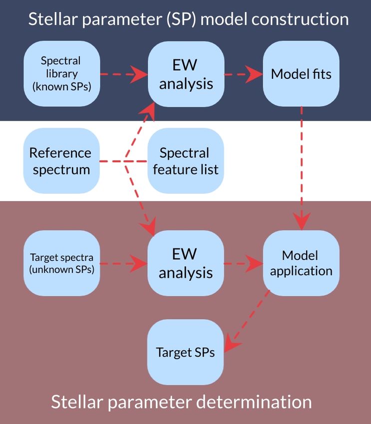
2 C. Lehmann et al.
spectra of candidate stars and the solar spectrum to identify solar as it can obtain 392 spectra simultaneously at a moderate resolving
twins. Their results inspired the differential approach that is used in power ( ≈ 28,000). Nevertheless, Sun-like stars at 4 kpc will only
this work. result in / ∼ 5 per pixel spectra in 1 h of observation. We will
 The motivation for our Survey for Distant Solar Twins (SDST) combine HERMES spectra from consecutive nights to improve the
is to discover solar twins as probes for possible variations in the / of our distant targets to ∼ 25 per pixel. Therefore, our aim
strength of electromagnetism – the fine-structure constant – across was to develop a method to use these low / combined HER-
our Galaxy (Murphy et al. in prep; Berke et al. 2022a, b; in prep). MES spectra to confirm distant solar analogues with a precision of
Stars closer to the Galactic centre sample regions of higher dark ( eff , log , [Fe/H]) ∼
 < (100 K, 0.2 dex, 0.1 dex).
matter density, and so our project aims to test for any fundamen- We present a novel approach to identify solar twins and analogues
tal, beyond-Standard-Model connections between electromagnetism optimised to work with HERMES spectra. We model the EWs of
and dark matter. Such connections are proposed within some theo- spectral absorption features as functions of their stellar parameters.
retical models of fundamental physics (e.g. Olive & Pospelov 2002; The method has two major advantages:
Eichhorn et al. 2018; Davoudiasl & Giardino 2019). However, all
 (i) It leverages existing spectral data from the Galactic Archae-
currently known solar twins are close to our solar system (within
 ology with HERMES (GALAH) survey (Martell et al. 2017;
800 pc) because more distant stars would be too faint to have been
 Buder et al. 2018) to create models for absorption features. The
useful for other astrophysical studies. This raises a key challenge: the
 library of stacked spectra from Zwitter et al. (2018) provides
need to identify and spectroscopically confirm solar twins at large
 > 800 pc, i.e. with magnitudes > 15 mag. sample spectra with high / (if not otherwise specified we
distances ∼ ∼ use signal-to-noise per pixel within this work) and HERMES
 Berke et al. (2022a; in prep) and Murphy et al. (in prep) recently
 resolution on a grid of varying stellar parameters, which is
demonstrated that solar twins can be used to constrain variation
 ideal to create this model.
in , at a level of precision two orders of magnitude better than
 (ii) The method operates fully differentially with respect to a high
current astronomical tests. Their method is measuring absorption
 precision solar spectrum (Chance & Kurucz 2010). Specifi-
line separations with high precision to constrain the variation of 
 cally, the reference spectrum is used to homogenise the pro-
between target stars. Solar twins are ideal for this purpose as we can
 cesses of continuum normalisation and radial velocity correc-
compare them both with each other, the Sun and local, close-by solar
 tion on a line-by-line basis. This ensures that a line’s EW is
twins without introducing additional systematic effects. We use the
 measured in the same way for all target spectra and, therefore,
stellar atmospheric parameters, eff , [Fe/H] and log , together as a
 differences between stars can be reliably traced.
proxy to determine how Sun-like a solar twin is.
 We adopt the following definitions of solar twins and solar ana- These advantages make it possible to measure the stellar pa-
logues from Berke et al. (2022b; in prep): rameters eff , [Fe/H] and log with low uncertainties while
 
  eff ± 100 K, also minimising computation time, i.e. ( eff , log , [Fe/H]) ≈
 (50 K, 0.08 dex, 0.03 dex) for / = 25 per 0.063 Å pixel in ∼
 < 10 s
 
 
 Solar twin = log ± 0.2 dex, (1)
  [Fe/H] ± 0.1 dex,
  per star.
 
 This paper is structured as follows. In Section 2 we present our
 
 
 
  eff ± 300 K, algorithm for solar analogue identification in detail. In Section 3
Solar analogue = log ± 0.4 dex, (2) we describe the results of our method when applied to the solar
  [Fe/H] ± 0.3 dex
 
  reference spectrum (Chance & Kurucz 2010) as well as spectral data
where we use the following values for solar stellar parameters: from AAT/HERMES and HARPS at the ESO 3.6 m telescope in
( eff , log , [Fe/H] ) = (5772 K, 4.44 dex, 0.0 dex) (Prša et al. La Silla, Chile. In Section 4 we discuss the impact of this method
2016). Note that these definitions do differ in the literature, e.g. on the project to map out the fine-structure constant throughout
Cayrel de Strobel et al. (1981); Cayrel de Strobel & Bentolila (1989); the Milky Way and compare our method to other stellar parameter
Friel et al. (1993); Cayrel de Strobel (1996) defined solar twins using measurement algorithms in the literature. Section 5 concludes and
the same three stellar parameters above but with narrower ranges as summarises the paper.
well as restrictions on other physical parameters like age, microtur-
bulence, chemical composition, etc. Such narrow definitions are not
practical for our search because of how unlikely it is to find such
 2 EPIC STELLAR PARAMETER MEASUREMENT
a perfect match to the Sun. For the same reason, other studies (e.g.
de Mello et al. 2014) defined the term ‘solar analogue’ as stars that We developed the ‘EPIC’ (EW comParIson Code) algorithm to deter-
are less Sun-like than solar twins and therefore easier to identify as mine stellar parameters in low / ∼ 25 spectra of solar analogue
well as more practical. Berke et al. (2022b; in prep.) demonstrated stars (henceforth ‘target spectra’) with moderate resolving power
that solar analogues, as defined in equation (2), are reliable probes (20,000 . . 28,000). The EPIC code is publicly available on-
of variations in the fine-structure constant between stars, so they are line in Lehmann et al. (2022). EPIC analyses a predetermined set of
the prime targets of our survey. absorption features (Section 2.2) to measure the stellar atmospheric
 The goal of the SDST is to identify a large number of solar ana- parameters, i.e. effective temperature eff , surface gravity log and
logues (between 200 and 300, after initial photometric pre-selection metallicity [Fe/H], in target stars. We utilise two techniques to min-
of ∼600), up to ∼ 4 kpc away, using medium-resolution spectroscopy. imise uncertainties and improve efficiency in this method: (i) We
The ∼40–50 most Sun-like of these, spread across several distance use a set of high-quality library spectra to determine the sensitivity
bins, can then be followed-up with high-precision spectrographs to of absorption line EWs to the stellar parameters. (ii) We measure
provide accurate measurements of the fine-structure constant. The the EWs in a fully differential manner with respect to a high-quality
High Efficiency and Resolution Multi-Element Spectrograph (HER- reference spectrum with well-known stellar parameters.
MES) at the 3.9 m Anglo-Australian Telescope (AAT) is ideal for the Figure 1 visualises the overall approach which we split into two
purpose of spectroscopically confirming solar analogue candidates different operation modes:

MNRAS 000, 1–16 (2022)

SDST I: EPIC stellar parameters 3
 • Blue (B): 4713–4901 Å
 • Green (V): 5649–5872 Å
 • Red (R): 6478–6736 Å
 • Infra-Red (IR): 7585–7885 Å.
 The combination of mirror size, multiplexing and resolving power
 allow the acquisition of / ∼ > 25 (in the red CCD) spectra of Sun-
 like stars at distances up to ∼ 4 kpc which should enable us to measure
 spectral stellar parameters with adequate precision. Furthermore, a
 crucial advantage of HERMES for identifying solar analogues at
 such large distances is the availability of the spectral library (Zwitter
 et al. 2018) established by the GALAH survey (Martell et al. 2017).
 They stacked 336,215 GALAH spectra into bins spanning a wide
 range of the three stellar atmospheric parameters. These stacked
 spectra have high / so that, for the purposes of this work, they
 are effectively noiseless and have a resolving power almost identical
 to (though slightly lower than) individual HERMES spectra. This
 spectral library makes it possible to establish a model connecting
 differences in EWs between absorption features in reference and
 target spectra to stellar parameters. In this section, we describe our
 application of the EPIC approach to HERMES spectra.

 2.1 Preparing spectra for EPIC
 We prepare different spectral datasets so that the EPIC algorithm can
Figure 1. Schematic of overall approach used in EPIC to measure stellar be applied. Several different input spectra are required: a reference
parameters (SP) of target star spectra using differential equivalent width (EW) spectrum, target spectra, and stacked (i.e. library) spectra. Addition-
measurements. The white central area contains the essential reference inputs ally, we created an algorithm which can prepare non-HERMES high
on which the method relies, while the blue area represents the SP model resolution spectra so that they can be analysed by EPIC as if they were
construction mode and the red area the SP determination mode. We explain HERMES spectra. We describe below how each type of spectrum is
this approach in detail in Section 2. prepared for use in EPIC.

 (i) Stellar parameter model construction: EPIC measures the 2.1.1 Reference spectrum
 EWs of a list of absorption features in a set of library spectra.
 We determine the difference in EW with respect to a high / A high / , high-resolution spectrum is used as a reference. When
 reference spectrum. The variation of EW differences in each searching for solar analogues, we utilise the solar atlas (‘KPNO2010’)
 feature is modelled as a simple polynomial function of the from Chance & Kurucz (2010) as our default reference spectrum. It
 three stellar atmospheric parameters (Section 2.5). The library covers all four HERMES bands (wavelength range of 2990–10010 Å),
 must comprise high / spectra with similar resolving power is effectively noiseless for our use, has a high resolving power ( =
 as the target spectra and must have precisely determined stellar 200,000–300,000) and is corrected for telluric absorption.
 parameters. We next prepare the reference spectrum for comparison with the
 (ii) Stellar parameter determination: Using the model estab- HERMES data. The first step is to cut it into the four wavelength
 lished in (i), EPIC determines the stellar parameters of target ranges (also called ‘bands’) that are covered by HERMES. We include
 spectra. The EWs are measured with respect to the same ref- a 20 Å wider wavelength range on both ends of each band as a
 erence spectrum used for model construction. EPIC then finds buffer to avoid edge effects in subsequent steps, i.e. the convolution
 the best fit of the individual target EWs to the model to deter- to HERMES resolution. We then project the wavelength grid from
 mine stellar parameters. the original spectrum onto a new version with constant wavelength
 spacing using the SpectRes (Carnall 2017) Python package. The
 The precision for measured stellar parameters depends on several wavelength grid is still very fine after this step compared to HERMES
factors: the / of the target spectrum, systematic errors in the EWs, spectra (pixel-width ∼ 0.01 Å).
how well the model fits the library and target EW measurements, as Next, we normalise the spectrum by identifying continuum regions
well as the choice of spectral features in the line list. We focused con- and fitting a polynomial of flux versus wavelength. The first part of
siderable effort on addressing these possible origins of uncertainty the normalisation process is to cut each band into overlapping sub-
and emphasise them within the detailed method explanation below. spectra (Fig. 2 illustrates this step). This is done to simplify the
 While the outlined approach could, in principle, be applied to normalisation as we can now calculate the local continuum on each
any spectrum from a wide range of different instruments, we fo- sub-spectrum independently. We mask out the hydrogen absorption
cus on HERMES in this paper. HERMES (Sheinis et al. 2015) is a (4855 ≤ ≤ 4870 Å and 6555 ≤ ≤ 6575 Å) and strong telluric
multi-object spectrograph mounted on the 3.9 m AAT, fed by 392 de- features (7587 ≤ ≤ 7689 Å) because the algorithm would identify
ployable fibres via the 2-degree-field (2dF) unit. It achieves moderate pixels within these wide emission/absorption areas as part of the
resolving power ( ∼ 28,000) in four relatively narrow wavelength continuum. We also mask any pixels that are more than 2.5 times
bands, each recorded in a different arm of the instrument: the median flux in each selected sub-spectrum to initially select

 MNRAS 000, 1–16 (2022)

4 C. Lehmann et al.
 stellar absorption feature (Section 2.3.4) so this initial normalisation
 does not need to be perfect. Furthermore, we identified sky emission
 features that tend not to be well corrected and interfere with the sub-
 1000 sequent preparation process in Section 2.3. We normalise a non-sky
 subtracted version of the target spectrum which makes identification
Counts [ADU]

 of emission features trivial and remove pixels within 30 km s−1 of
 sky emission from all further analysis.
 We need to correct the radial velocity of a target spectrum to
 the zero-velocity frame of the reference spectrum. We selected a
 500
 1600 km s−1 velocity range in each band of HERMES centred on
 these four wavelengths: 4807, 5763, 6670 and 7818 Å. These were
 HERMES spectrum chosen because they are surrounded by a relatively large number
 Continuum fit of stellar absorption features, which is ideal for a cross-correlation.
 4750 4800 4850 4900 We cut out the corresponding wavelength range in the reference and
 Wavelength [Å] target spectra and reduce the resolving power of the reference sub-
 spectrum to match the target spectrum (Section 2.3.3 for details).
Figure 2. B-band in a representative high- / HERMES spectrum from the
GALAH survey. The black arrows mark the overlapping sub-spectra that we
 The 1600 km s−1 sections of the reference and target spectra are then
derive the normalisation from. The orange dashed line shows the resulting cross-correlated to find the radial velocity shift between them. We
continuum after the local sub-continua are combined. apply the correction as a constant shift in wavelength to the whole
 band to keep a constant pixel wavelength spacing, as opposed to a
 more precise wavelength dependent radial velocity correction. This
against strong cosmic rays (this is relevant when normalising non- makes it only precise to ∼ 1−2 HERMES pixels, which is sufficiently
reference spectra; see Section 2.1.2). We remove pixels with the accurate for our purposes as we later apply an additional line-by-line
lowest 75% of fluxes to select against absorption lines in each sub- correction for the radial velocity (Section 2.3.1).
spectrum and fit a third-order Legendre polynomial to those that
remain. We calculate the standard deviation of these fluxes from the
fit and select against those > 3 standard deviations above and > 1.5
standard deviations below the fit. The fit and deselection process is 2.1.3 Library/stacked spectra
repeated until the number of pixels remains constant. The final fit The stacked spectra of Zwitter et al. (2018), which are used as a
represents the calculated continuum of the sub-spectrum. We join spectral library to create the model in Section 2.5, need to undergo
the sub-continua together by weighting each sub-continuum linearly the same normalisation and radial velocity correction steps as the
in the overlapping regions; the continuum closest to the centre of an target HERMES spectra (Section 2.1.2). Additionally, we need to
individual sub-spectrum has close to 100% weight while the edges create an error array for these spectra so that we can later create a
have close to 0% weight. This creates a continuum approximation for realistic pixel weight array for individual
 √ absorption features (Section
the full wavelength band. We normalise by dividing each pixel by its 2.4). Any error array proportional to flux simulates a real error array
respective continuum value. well enough for this purpose. Furthermore, we re-sample the stacked
 Note that, at the end of the reference spectrum preparation, the spectra to a grid with 4096 pixels per band and constant pixel width
resolving power is not reduced as the desired resolving power is a using SpectRes to closely match the properties of HERMES spectra.
function of both the target spectrum and the wavelength (Section
2.3). Furthermore, if a different reference spectrum is used in EPIC,
a different stellar parameter model (Section 2.5) must be created.
This is because the EW analysis is differential, and hence dependent 2.1.4 High resolution target spectra
on the reference used. High resolution target spectra are primarily used for testing purposes
 in EPIC. The spectral data can be obtained from any instrument with
 higher resolving power than HERMES ( > 28,000). We primarily
2.1.2 Target spectra use spectra from ESO’s (European Southern Observatory) HARPS
The target stars observed with HERMES are the main focus of this spectrograph (High Accuracy Radial velocity Planet Searcher) as the
work. To discover new, distant solar analogues, we need to use HER- data are easily accessible from the ESO Science Archive and the
MES spectra with / & 25 per pixel and measure stellar parameters instrument has accumulated a large number of high / spectra over
 < (100 K, 0.2 dex, 0.1 dex).
with a precision of ( eff , log , [Fe/H]) ∼ almost 20 years of operation. We only use spectra with / ∼ > 50 per
 We start the preparation of these spectra with the same normali- 0.8 km s−1 pixel, which further increases by a factor of ∼ 2 when
sation process described above (Section 2.1.1). The only difference they are convolved and down-sampled to match HERMES resolution
in application is that we need wider masked wavelength regions for and sampling, so we can safely assume these spectra to be noiseless
hydrogen lines and telluric absorption because the radial velocity of for the purpose of our tests.
these spectra is unknown at this point of the analysis. We adjusted The preparation of these spectra involves steps already explained
each mask to accommodate a 250 km s−1 maximum radial veloc- in Section 2.1.1 and 2.1.2, i.e. converting the wavelength range to
ity (and barycentric velocity) based on expected radial velocities of HERMES wavelength bands, normalising the spectrum and correct-
stars closer to the Galactic Centre. These larger masks potentially ing for radial velocity. Note that the infrared wavelength region is not
cause issues for the continuum fit of individual sub-spectra but they covered by HARPS, so we are left with only the blue, green and red
can be avoided with correct sub-spectrum positioning, i.e. hydrogen bands. In contrast to Section 2.1.1, these are intended to be used as
lines and telluric features should not be on the edge of sub-spectra. target spectra, so we have to reduce their resolving power to match
Note that we apply a more precise local normalisation around each that of HERMES. So we convolve each band with a Gaussian kernel

MNRAS 000, 1–16 (2022)

SDST I: EPIC stellar parameters 5
that reduces the resolving power to 28,000. The convolution process 1.0
is detailed in Section 2.3.3.

 Normalized flux
 0.8
2.2 Selection of absorption features
The list of stellar absorption features (‘line list’) used in this work
is specialised for solar analogue spectra from the HERMES spec- 0.6
 Reference spectrum
trograph. We included lines from two previous line lists: the first Reference Centroid
was used by Datson et al. (2015) specifically to help identify solar Line list wavelength
analogue stars — 82 absorption lines from this list were available 0.4 6595.0 6595.5 6596.0
within the HERMES wavelength range; the second line list was used 1.0
by the GALAH survey (Buder et al. 2018) and provides 216 absorp-
tion lines that are useful to determine stellar atmospheric parameters.

 Normalized flux
Note that 44 features were present in both lists. 0.8
 Additionally, we visually selected other features within the HER-
MES wavelength bands that were not included in either of these lists,
which contributed another 54 absorption features for a total of 308. 0.6
Of these lines, we selected only those matching the following crite- Unconvolved reference
 Convolved reference
ria, each applied to the features as they appear in the solar reference HERMES target
spectrum at HERMES resolution (unless otherwise specified): 0.4 6595.0 6595.5 6596.0
 Wavelength [Å]
 (i) We check if the feature is useful in a low / (∼ 25) HERMES
 spectrum. Our measurements indicate that the typical uncer- 1.0
 tainty for EWs in such a spectrum is EW ∼1 mÅ. We calculate
 the EW of each line and remove those with EW≤ 5 mÅ from Normalized flux
 the list. 0.8
 (ii) The features should not be saturated, so we visually determine
 if a line is saturated or close to saturation and remove them from
 the list. For this selection we make use of the high resolution 0.6
 Pre-norm target
 ( = 200,000–300,000) solar atlas (Chance & Kurucz 2010). Post-norm target
 We defined saturation in a line as absorbing more than 80% of Reference
 0.4 6590 6595 6600
 the normalised flux at its centre.
 (iii) We reject features that appear to be blended with other fea- 1.0
 tures. This is done by visual inspection as it does not need to
 be rigorously defined. Blends can lead to more complicated
 Normalized flux

 behaviour with respect to stellar parameters, so we also select 0.8
 against them in the residual based selection below.
 (iv) We avoid features that are close (∼ 50 km s−1 ) to telluric ab-
 sorption to avoid atmospheric influences. 0.6
 Reference
A feature’s EW also needs to show simple behaviour with respect to HERMES target
 Weights
changing stellar parameters so that we can establish a model for it –
 0.4 6595.0 6595.5 6596.0
see Section 2.5. We inspected residuals between the model and test
 Wavelength [Å]
data and determined that lines with average residuals of more than
2% of their full EW range are filtered out. This leaves us with 125 Figure 3. Line preparation and EW measurement in EPIC. The top panel
absorption features in the line list. shows the line centering. The algorithm searches for the lowest flux value in
 We chose to apply the above criteria less strictly to ionised lines the local environment of the reference spectrum with sub-pixel precision (Sec-
– i.e. average residuals can have up to 3% of the line’s full EW tion 2.3.2). The black dotted vertical line shows the line list information and
range. This is done because ionised lines are more sensitive to the the solid black line is our newly determined line centroid. The second panel
surface gravity than neutral lines, so our aim was to increase the visualises the resolving power matching and wavelength grid re-sampling of
 the reference solar spectrum to the HERMES target spectrum (Section 2.3.3).
method’s overall sensitivity to differences in log between stars.
 The third panel shows the re-normalisation process for the target spectrum,
This means that we extended the line list by an additional 6 ionised which matches the continuum flux with the reference (effect exaggerated for
lines (from 125 to 131 total lines). When comparing the application visual purposes; Section 2.3.4). The bottom panel shows the EW window
of the EPIC algorithm with and without these additional lines the (red dashed lines) and weighting of each pixel for the EW measurement (blue
resulting uncertainties for all stellar parameters are reduced: eff line, Section 2.4).
by 2%, [Fe/H] by 2.5% and log by 7% with the additional
ionised lines. Our final line list of 131 features is provided in Table
A1.

2.3 Line preparation
In this section, we describe how the wavelength area around each consistently in the library/stacked and target spectra. Each line is
spectral feature is prepared so that EW measurements can be made analysed independently in each spectrum.

 MNRAS 000, 1–16 (2022)

6 C. Lehmann et al.
2.3.1 Precise radial velocity correction We choose a wavelength area around the absorption line with a
 width of 800 km s−1 . This window is chosen to be large because it
We determined the radial velocity using a 1,600 km s−1 window in
 allows a noise-resistant, precise matching of the target continuum
each band as part of the spectral preparation (Section 2.1.2), but we
 to the reference one. However, it is limited to this size so that it is
need to ensure that each absorption feature in the reference and target
 not sensitive to poor initial continuum fits. Additionally, this wave-
spectrum is aligned to minimise EW systematic errors. In this step
 length space determines how close to the edge of a spectral band our
we make a more precise local radial velocity correction for each line
 absorption features can be, i.e. not closer than 800 km s−1 as to not
of interest. For a comparatively small velocity window of 380 km s−1
 affect this process.
around the line, we re-sample the target or stacked spectrum using
 For convenience, we first re-normalise the reference spectrum by
SpectRes to match the wavelength grid of the reference spectrum.
 the maximum flux in the chosen window. The high / reference
This allows us to gain sub-HERMES pixel precision in the new
 spectrum is not affected by any cosmic rays and has a precise sky
correction. We apply the same cross-correlation process from Section
 subtraction of telluric emission, so this straight forward approach is
2.1.2 to this small wavelength section of re-sampled target or stacked
 sufficient.
spectrum to calculate the radial velocity differences between the
 Next, EPIC adjusts the average target spectrum flux to that of the
reference and target absorption feature, which is then corrected for.
 re-normalised version of the reference in the same wavelength region
 around the absorption line (i.e. 800 km s−1 ). We remove the 75% of
2.3.2 Line centering pixels with the lowest flux values in the reference spectrum from both
 the target and the reference in order to ignore absorption lines in this
We need to determine the precise absorption line centre so that we process (note that their wavelength grids are identical at this point in
can define the wavelength window for the EW measurement. We the analysis). Additionally, we remove the 30 km s−1 window around
use the wavelength values in the line list as a starting point for this the line centroid used for the EW measurement (Section 2.4). A
determination. The top panel of Fig. 3 shows an example line for weight is assigned to all remaining pixels, given by their inverse flux
which we determined the line centre. variance in the target spectrum. We determine the weighted mean
 The absorption features of reference and target spectrum are flux of all remaining pixels in both the reference and target spectrum.
aligned with each other after the previous step so we only need The target spectrum is then scaled by the ratio of these weighted
to determine the line centre for one of them. We choose to determine means. This method of normalisation aligns the continuum of the
the line centroid in the reference spectrum to avoid noise. We define target spectrum very precisely with the reference around the desired
a small wavelength window of 16 km s−1 around the line list wave- absorption line.
length for the feature. This window is chosen as a little more than half
the full width at half maximum (FWHM) at HERMES resolution and
assumes that the line list wavelength is within the absorption feature.
We identify the line centroid as the minimum of a quadratic fit to the 2.4 Equivalent width measurement
three pixels with the lowest flux value within the chosen window. After the preparation steps in Section 2.1 and 2.3, we can define a
 window of 30 km s−1 around the line centroid in which to measure the
 EW. This window is optimised to include most of the absorption of
2.3.3 Resolving power reduction and reference re-sampling
 the feature while minimising the influence of potential weak blending
We reduce the resolving power of the reference spectrum to match effects (lines with strong blending were excluded in Section 2.2).
the target spectrum, as visualised in the second panel of Fig. 3. As We determine a weight for each pixel,
noted in Section 2.1.1 the reference spectrum has a high resolving
 
power (i.e. = 200,000–300,000) so we convolve it with a Gaussian = , (3)
with a FWHM corresponding to HERMES spectra. We adjust the 2
FWHM to take the finite of the reference spectrum into account. where is the uncertainty of the flux and is the fraction of the
Importantly, HERMES does not have a constant resolving power as pixel-width within the defined wavelength window. That is, pixels
a function of wavelength (Kos et al. 2017), so we need to determine fully within the line definition have = 1, pixels fully outside have
the resolving power for each line separately. We do this by using the = 0 and pixels partially within have 0 < < 1. A typical weight
current version of the GALAH resolving power maps which provide distribution is visualised in the bottom panel of Fig. 3. These weights
 for all HERMES fibres as functions of wavelength (see section 7 are derived with the flux uncertainties in the target spectrum but
in Kos et al. 2017). Note that the original, observed wavelength was applied to both the target and reference spectrum to maximise the
used to find the corresponding value in the map, not the radial comparability between the two.
velocity corrected value. With a weight attached to every pixel, we can calculate the nor-
 Furthermore, we need the reference spectrum wavelength grid to malised absorption and the EW of the line via
match that of the target spectrum, so after the convolution is applied Í
we use SpectRes to re-sample the reference spectrum to the target or 
 © 
 =1−­ Í
stacked spectrum’s wavelength grid. ª
 ®, (4)
 
 « ¬
2.3.4 Continuum re-normalisation = , (5)

We re-normalise the target/stacked spectrum locally to ensure that its where is the normalised and weighted average absorption, the
continuum matches the reference spectrum’s as closely as possible. width of the defined wavelength window and the flux in an in-
This improves upon the initial continuum in the spectral preparation dividual pixel normalised to 1. For the selected absorption features,
(Section 2.1.1). The third panel of Fig. 3 visualises the effect of this we use the difference between their EW and that in the reference
step. spectrum, EW, in further analysis to measure the stellar parameters.

MNRAS 000, 1–16 (2022)

SDST I: EPIC stellar parameters 7
 for spectra within a bin instead of the central value of the bin in
 our calculations. This is necessary as stellar parameters are not uni-
 log(g) = 3.8
 20 formly distributed within a bin, e.g. more spectra within GALAH
 DR2 have log = 4.3 – 4.4 dex than log = 4.4 – 4.5 dex meaning
 log(g) = 4.2 a stacked spectrum combined from all those spectra will have an
 effective surface gravity log < 4.4 dex while the bin is labelled as
 δ EW[mÅ]

 log = 4.4 dex. While we have chosen to use the weighted mean val-
 0 log(g) = 4.6 ues here, we also conducted the calibration process using the median
 instead, and found that the resulting stellar parameters for target stars
 differ by ( eff , log , [Fe/H]) . (2 K, 0.005 dex, 0.001 dex), which
 are negligible compared to our other sources of error.
 −20 With these spectra we can create a model for each individual
 feature within the line list. Each model has different parameters
 ( ), which are used to connect effective temperature eff , surface
 gravity log and metallicity [Fe/H] to varying EW. We attempt
 −40 to maximise the model’s ability to reproduce the training set while
 5500 6000 using the simplest formula for a fitting approach:
 [Fe/H] = −0.5 2
 = 0 + 1 eff + 2 eff + 3 log + 4 log 2
 20 [Fe/H]
 + 5 [Fe/H] + 6 [Fe/H] 2 + 7 (6)
 [Fe/H] = −0.3 eff
 where are the model constants for an individual line. We visualise
 δ EW[mÅ]

 0 the model creation in Fig. 4 which shows a single transition for
 which we measured EWs in stacked spectra. We tried several different
 [Fe/H] = −0.1 [Fe/H] = 0.1 model formulas to fit the measurements and found that second order
 moments and a cross term between [Fe/H] and eff improved our
 results. Additional terms, including cross-terms involving log , had
 −20 [Fe/H] = 0.3 a negligible effect on our results and added instability to the method.
 We determined the EWs for all absorption features within our
 line list for all available stacked spectra that have stellar parameters
 within a initially broad range around solar values, i.e. eff = 5800 K±
 −40 700 K, log = 4.4 dex ± 0.6 dex and [Fe/H] = 0.0 dex ± 0.5 dex. It
 5500 6000 is possible to extend the model boundaries (e.g. to eff = 5800 K ±
 Temperature[K] 1400 K), but we would need to use a more complex model than
 equation (6) to avoid systematic errors and more available stacked
Figure 4. Stellar parameter model for eff of a single transition (Fe I at spectra to cover that range. We can solve equation (6) for all to
4892.86 Å). The plot shows slices of a four dimensional fit of the three stellar connect EWs to stellar parameters for each line. This is done via a fit
atmospheric parameters to the EW differences (between the stacked spectra for these parameters that is based on the measurement of EWs and
and the solar reference spectrum). The top panel has constant [Fe/H] = 0.0 dex the stellar parameters that are already known for the stacked spectra.
while the bottom panel has constant log = 4.4 dex. The solid lines represent With these model parameters we can calculate stellar parameters
the model fit while the dots are EW measurements for stacked spectra from for stars by reversing the procedure and solving for eff , log and
Zwitter et al. (2018). The colours correspond to constant values in log (top [Fe/H] in equation (6). When reversing the process, we perform a
panel) and [Fe/H] (bottom panel) as denoted close to each line.
 least squares fit to the EW values of all lines in a target spectrum,
 with inverse variance weighting which combines the uncertainties in
 the EW measurements and model values. The least squares fitting
2.5 Measuring stellar parameters
 provides the best-fit stellar parameters and the covariance matrix, the
Each stellar absorption line has a unique dependency on the stellar diagonal terms of which provide our quoted uncertainties.
parameters. The EPIC algorithm models these dependencies and uses In principle, it is possible to extend the number of stellar pa-
them to measure stellar parameters via EWs. rameters that are measured by the model (e.g. by specific metal
 First, we require a set of spectra with known stellar parameters abundances), but there are several points against this. First, the un-
in order to determine the coefficients of the model (see equation certainty would increase for all stellar parameters and parameters.
(6)). The GALAH survey provided medians of observed spectra Furthermore, we would need a complete set of spectra which have
(Zwitter et al. 2018) with a wide range of stellar parameters; ideal these parameters calculated as a base for further analysis. So it is not
for the purpose of model creation. These spectra were made from practical at the current time to expand the algorithm this way.
spectra in GALAH DR2 (Buder et al. 2018). The stellar parameters
of the initial spectra have been determined by The Cannon (Ness
 2.6 Stellar parameter calibration
et al. 2015) and sorted into bins by their effective temperature, sur-
face gravity and metallicity (Zwitter et al. 2018). The size of these The stellar parameters calculated with EPIC inherit any potential
bins in stellar parameter space is eff = 50 K, log = 0.2 dex (g systematic errors from the stacked spectra (Zwitter et al. 2018) and
in cm/s2 ) and [Fe/H] = 0.1 dex. All spectra within the same bin their calibration from The Cannon (Ness et al. 2015). Therefore, we
were stacked to create high / model spectra with known aver- need to investigate and correct systematic effects if present. First, we
age stellar parameters. We use the weighted mean stellar parameters found differences between EPIC’s stellar parameters measured for

 MNRAS 000, 1–16 (2022)

8 C. Lehmann et al.
solar spectra and their literature values for the Sun. We implemented
a ‘reference-point correction’ for this (see Section 3.1 for details).
Additionally, we investigated stellar parameter dependent differences 5760 solar
between EPIC’s estimated values and stellar parameters measured

 Teff[K]
from high resolution and high / echelle spectroscopy (Casali et al.
2020). In addition to the ‘reference-point correction’ we perform a
‘higher-order correction’ to account for stellar parameter dependent 5720
systematic errors (see Section 3.3 for details). This enables us to
switch from an initial calibration based on the spectral library to one
that agrees more with stellar parameters determined in Casali et al.
(2020). 5680
 For all of these calibrations we use spectra with simulated error ar- 4.44 SA HA H1 H2 H3 H4
rays using values corresponding to S/N = 50 per pixel in all HERMES
bands. This provides a reasonably realistic relative weighting of the
flux and model errors in the EWs when fitting the model. Using a very 4.40

 log(g)
large / would have left the model errors to dominate. So, instead,
we chose a / that is more typical of the real HERMES spectra
we will normally apply EPIC to. The stellar parameters change very 4.36
little as a function of this chosen S/N in the range 20–100 per pixel:
 ( eff , log , [Fe/H]) = (3 K, 0.002 dex, 0.0008 dex). If spectra of
higher / are to be analysed, EPIC would need re-calibration or, in 4.32
future versions, possibly a / -dependent calibration.
 SA HA H1 H2 H3 H4
 0.02
3 RESULTS
 0.01
 [Fe/H]
We applied EPIC to spectral data to test and refine the calibration, and
present the full capability of the method. We describe the results of the 0.00
algorithm for the following data products: the solar reference spec-
trum (Chance & Kurucz 2010) and solar spectra obtained from col- −0.01
lecting reflected light from minor solar system bodies – Ganymede,
Ceres and the Moon – from HARPS (Mayor et al. 2003), spectra −0.02
from HARPS for which precise stellar parameters have been mea-
sured (Casali et al. 2020) and HERMES spectra from the GALAH SA HA H1 H2 H3 H4
Data Release 2 catalogue (Buder et al. 2018).
 Figure 5. EPIC uncalibrated stellar parameter measurements for solar spectra.
 This figure shows results for the following solar spectra, each analysed with
3.1 Solar spectra: reference-point correction
 the HARPS version of our line list (i.e. excluding absorption features marked
The main function of EPIC is to measure stellar parameters, so it with an asterisk in Table A1): SA: solar atlas (Chance & Kurucz 2010); H1-
is important to test if measured parameters match their literature 4: HARPS spectra obtained by observing reflected light from minor bodies
 satellites (H1: Ceres observed in 2006; H2: Ganymede in 2007; H3: the Moon
values for selected test targets. Naturally, the first test is to repro-
 in 2008; H4: Ceres in 2009); HA: mean value of H1-4 weighed by their inverse
duce stellar parameters of the Sun as it is the main reference for
 variance.
our method. We apply EPIC to the solar atlas used as our main
reference (Chance & Kurucz 2010) which is prepared as a refer-
ence (Section 2.1.1) and a target (Section 2.1.4) spectrum for this eff in GALAH (DR2) and that derived via the infrared flux method
analysis. We derived stellar parameters using the EPIC algorithm (Casagrande et al. 2010, 2014) using SkyMapper photometry.
and find that the values calculated for the solar atlas ( eff , log , As a second test, we compare the stellar parameters measured for
[Fe/H]= 5711 ± 7 K, 4.38 ± 0.01 dex, 0.004 ± 0.005 dex) are offset the solar atlas to those we measured for another set of solar spectra to
from the current IAU standard values for solar stellar parameters verify the ‘reference-point correction’. We utilise the archive of the
( eff , log , [Fe/H] ) = (5772 K, 4.44 dex, 0.0 dex) in Prša et al. HARPS spectrograph, i.e. their reflected solar spectra from Ceres,
(2016) by Δ( eff , log , [Fe/H]) = (61 K, 0.06 dex, −0.004 dex). We Ganymede and the Moon. These are high resolution spectra with high
are able to trace these offsets back to the initial stellar parameter / that can easily be convolved to HERMES resolution (Section
measurements of The Cannon which show systematic differences 2.1.4). A shortcoming of these spectra is that HARPS only covers the
when compared to other stellar parameter studies (e.g. Adibekyan wavelength ranges of the B, G and R bands in HERMES, so the IR
et al. 2017; Casali et al. 2020, more in Section 3.3 and Section band is not available. Another shortcoming is that the data pipeline
3.4). Therefore, we need to address this issue with a ‘reference- for HARPS does not provide a correction for telluric absorption.
point correction’. This process corrects the model (Section 2.5) by Therefore, we need to adjust the line list, removing features that can
adding constants to the stellar parameters of model spectra, i.e. we fall within the same wavelength range as telluric absorption due to
changed eff → eff + 61 K, log → log + 0.06 dex and [Fe/H] → stellar radial velocity differences and Earth’s barycentric velocity
[Fe/H] − 0.004 dex in equation (6). This corrects the measured solar variations. We considered a maximum radial velocity difference of
stellar parameters to their literature values. We note that Buder et al. 200 km s−1 for this alternative line list in order to accommodate the
(2018) found the same mean offset (61 K) between the spectroscopic HARPS spectra from Casali et al. (2020) considered in Section 3.3.

MNRAS 000, 1–16 (2022)

SDST I: EPIC stellar parameters 9
All features that we excluded for the analysis with HARPS spectra
are marked with an asterisk in Table A1. The purpose of this test is
 100

 ∆Teff[K]
to compare measured stellar parameters for the solar atlas (Chance
& Kurucz 2010) to those of the HARPS solar spectra, so we need
to apply the same analysis to both, i.e. we only analyse absorption 0
features for the solar atlas that can be used for HARPS spectra.
 The results of this analysis can be seen in Fig. −100
5. We identify a discrepancy, i.e. Δ( eff , log ,[Fe/H]) =
−11 K, −0.029 dex, −0.0140 dex, between stellar parameters mea- −200
sured for HARPS spectra and the solar atlas (HA and SA in Fig.
 5200 5600 6000 6400
5). We traced these differences back to slight changes in the normal-
isation process (Section 2.3.4) that are caused by very weak telluric
 Teff[K]
features that have not been removed in HARPS spectra. Additionally,
when analysing the solar atlas with and without an IR band, i.e. with
the reduced line list, we found negligible stellar parameter differ- 0.1

 ∆ log(g)
ences of Δ( eff , log ,[Fe/H]) = −0.6 K, −0.0003 dex, −0.0024 dex.
However, a missing IR band leads to an increase of ∼ 20% in un-
 0.0
certainties which is expected as the number of absorption features −0.1
declines. The same can be observed for other HERMES spectra.
 −0.2
3.2 Systematic effects between HERMES and HARPS −0.3
We used spectral data from the HARPS spectrograph in the process
 4.0 4.4 4.8
of testing EPIC (Section 2.1.4) which raises the question of whether log(g)
these spectra have systematically different stellar parameters than
HERMES spectra when measured with EPIC. We identified 18 target
stars that have been observed with both HERMES in GALAH DR2 0.05
 ∆[Fe/H]

as well as with HARPS in the ESO phase 3 database1 . We analysed
both the HERMES and the HARPS spectra for these target stars and
 0.00
compared their measured stellar parameters with each other. The −0.05
resulting stellar parameters and their differences are visualised in
Fig. 6. −0.10
 We found that the weighted average of GALAH-HARPS dif-
ferences are Δ( eff , log ,[Fe/H]) = (−10.9 ± 10.6 K, −0.021 ±
 −0.15
0.018 dex, −0.025 ± 0.007 dex). These systematic effects can explain −0.6 −0.3 0.0 0.3
the differences that we see between stellar parameters calculated for [Fe/H]
the solar atlas and the HARPS solar spectra observed from reflected
light (Section 3.1). The most likely source for these differences is Figure 6. Differences between EPIC results when using HERMES spectra
that HARPS spectra are not corrected for telluric features while both compared to HARPS spectra. The three panels show the effective temperature,
GALAH spectra and the solar atlas are corrected for telluric absorp- surface gravity (g in cm/s2 ) and metallicity. The y-axis shows the difference of
tion/emission. We expect this to influence the normalisation process these parameters between HARPS and HERMES spectra for the same target
 stars. The y-error-bars are combined from both the HERMES and HARPS
of EPIC (Section 2.3.4). We use HARPS spectra to re-calibrate EPIC
 uncertainties. The x-axis is the respective stellar parameter as measured for
with a ‘higher-order correction’ in Section 3.3 so there is the possibil- the HARPS spectra with EPIC. The ‘reference-point correction’ has been
ity of small systematic effects in the stellar parameter measurements. applied prior to this analysis while the ‘higher-order correction’ (Section 3.3)
However, only the linear and higher-order terms of this correction has yet to be applied.
are used, so this should be a very small effect, while the ‘reference-
point correction’ is based on the solar atlas which means that these
systematic effects would be reduced, especially for solar analogue ([Fe/H]) = 0.01 dex) and the calibration of eff , log and [Fe/H]
spectra. was done using the modelling process of the q2 algorithm (Ramírez
 et al. 2014). This provides an independently observed and analysed
 set of stars with well-determined stellar parameters which allows
3.3 Sun-like stars: higher-order correction us to test EPIC’s stellar parameter measurements. We gathered 458
After calibrating solar stellar parameters in EPIC we test the algo- spectra from HARPS for targets previously used in Casali et al.
rithm on a wider range of stars. Since we aim to minimise systematic (2020) from the ESO phase 3 database. This set of spectra was se-
errors for solar analogue stars (equation (2)) we need to find such tar- lected only by their availability in the archive, so we do not expect
gets in the literature to perform this test. Casali et al. (2020) provided additional systematic effects from the fact that not all 560 stars were
high precision stellar parameter estimations for 560 Sun-like targets used. We applied the EPIC algorithm, including the ‘reference-point
observed with the HARPS spectrograph. The uncertainties calcu- correction’, to these available data.
lated in this analysis are small ( ( eff ) = 10 K, (log ) = 0.03 dex, In the left three panels of Fig. 7 we can see how stellar parameters
 from the EPIC analysis compare to the higher-precision, independent
 values from Casali et al. (2020). These panels show systematic differ-
1 http://archive.eso.org/wdb/wdb/adp/phase3_spectral/form ences in eff and log that vary approximately linearly with the value

 MNRAS 000, 1–16 (2022)

10 C. Lehmann et al.

 Pre-Calibration Post-Calibration
 100
 ∆Teff[K]

 0

 −100
 5600 5700 5800 5900 5600 5700 5800 5900
 Teff[K] Teff[K]
 0.2
 ∆ log(g)

 0.0
 −0.2
 −0.4
 4.2 4.3 4.4 4.5 4.6 4.2 4.3 4.4 4.5 4.6
 log(g) log(g)
 0.1
 ∆ [Fe/H]

 0.0

 −0.1
 −0.4 −0.2 0.0 0.2 0.4 −0.4 −0.2 0.0 0.2 0.4
 [Fe/H] [Fe/H]
Figure 7. EPIC stellar parameter measurement compared to the analysis of Casali et al. (2020). The panels from top to bottom show the effective temperature,
surface gravity (g in cm/s2 ) and metallicity. The -axis represents the difference between stellar parameters calculated with EPIC and those of Casali et al.
(2020). The -axis shows the parameter as measured by Casali et al. (2020). The orange vertical lines represent solar values. The left panels show the differences
before the ‘higher-order correction’ and the right panels shows the improvement after we apply it.

of these parameters, while [Fe/H] seems to vary slightly non-linearly. substantially reduced in the right panels. This is because the system-
These systematic effects are visible because our initial calibration, atic effects described are not just dependent on the stellar parameter
based on The Cannon measurements, differs from the calibration of they are affecting, e.g. systematic effects in eff are also influenced
Casali et al. (2020). In order to match the stellar parameter calibra- by [Fe/H]. The scatter is reduced because these dependencies are ad-
tion of Casali et al. (2020), we need to correct for systematic effects dressed in equation (7). Therefore, we conclude that the systematic
that vary with respect to stellar parameters: we call this process a differences between our measured stellar parameters with EPIC and
‘higher-order correction’. We re-calibrate by fitting a polynomial of those from Casali et al. (2020) have been calibrated out, with a possi-
the following form to each of the stellar parameters, : ble exception at higher log values (i.e. log > 4.54 dex) which we
 need to be cautious of. Since EPIC’s calibration is fundamentally tied
 = 1, eff + 2, log + 3, [Fe/H] + 4, [Fe/H]2 , (7) to the analysis of Casali et al. (2020) it might need to be revisited in
where are the stellar parameter deviations between EPIC and the future as other works improve their stellar parameter calibrations.
Casali et al. (2020), eff and log are the effective temperature
and surface gravity differences with respect to the solar values (i.e.
 3.4 EPIC and GALAH/The Cannon
 eff = eff − 5772 K and log = log − 4.438) and , are the fit
parameters in the calibration process. This polynomial is subtracted EPIC currently focuses on measuring stellar parameters from HER-
from the measured stellar parameters to arrive at the final calibration MES spectra, so it is natural to compare its results with the GALAH
of EPIC. stellar parameter measurements derived from HERMES spectra us-
 The right panels of Fig. 7 visualise the effect of this process when ing The Cannon (Ness et al. 2015). EPIC was initially calibrated to
compared to the left panels. They show that EPIC’s stellar parameters The Cannon stellar parameters because the stacked spectra (Zwit-
(post-calibration) match the Casali et al. (2020) values within a small ter et al. 2018) combine many GALAH DR2 spectra whose pa-
uncertainty range. Additionally, the scatter seen in the left panels is rameters were calculated with The Cannon. Therefore, we expect

MNRAS 000, 1–16 (2022)

SDST I: EPIC stellar parameters 11

 Pre-Calibration Post-Calibration
 400
 ∆Teff[K]

 200
 0
 −200
 5200 5600 6000 5200 5600 6000
 Teff[K] Teff[K]
 0.6
 0.3
 ∆ log(g)

 0.0
 −0.3
 −0.6 4.0 4.2 4.4 4.6 4.0 4.2 4.4 4.6
 log(g) log(g)
 0.2
 ∆ [Fe/H]

 0.0

 −0.2
 −0.4 −0.2 0.0 0.2 0.4 −0.4 −0.2 0.0 0.2 0.4
 [Fe/H] [Fe/H]
Figure 8. EPIC stellar parameter measurement compared to the values provided in GALAH DR2 calculated with The Cannon (Ness et al. 2015). The panels
from top to bottom show the effective temperature, surface gravity (g in cm/s2 ) and metallicity. The -axes show the difference between EPIC’s stellar parameters
and The Cannon’s. The -axes show the parameters as measured with The Cannon. The vertical orange lines represent the solar values. The red horizontal
line highlights the ‘reference-point correction’ that has been applied to EPIC’s stellar parameters in all panels. The left panels show the differences before the
‘higher-order calibration’ while the right panels show them after that is applied.

pre-calibration stellar parameters from EPIC to agree with stellar tween EPIC’s and The Cannon’s stellar parameters pre-calibration
parameters in GALAH DR2. while the surface gravity seems to have a minor systematic effect
 We analysed a sub-set of GALAH DR2 with EPIC. These spectra which becomes most apparent at low and high log . A possible ex-
were selected from GALAH to have measured stellar parameters in planation for this systematic effect is that different choices for line
the following ranges: eff = [5200, 6400]K, log = [3.8, 5.0]dex lists affect the overall stellar parameter measurements, which is espe-
and [Fe/H] = [−0.5, 0.5]dex. Within these stellar parameter ranges, cially true for log . The dependence of absorption feature strengths
we randomly selected ∼ 1,858 spectra for a workable test data-set. – and therefore the precision of our measurements – on log varies
In this analysis we focused on GALAH’s second data release (DR2) on a line-by-line basis, so different choices of line list for EPIC can
(Buder et al. 2018) which is the basis for the stacked spectra (Zwitter lead to systematic effects as seen in Fig. 8. However, these offsets are
et al. 2018) we use for the model creation (Section 2.5). Figure small and will be calibrated out when doing the ‘higher-order correc-
8 shows EPIC’s stellar parameter values compared to those of the tion’ so it is not a major concern. Line-by-line differences in stellar
GALAH survey. We visualise EPIC’s stellar parameter estimation parameter dependence are present for eff and [Fe/H], but different
before (left three panels) and after (right three panels) the ‘higher- features generally follow the same qualitative trends for these param-
order calibration’. The ‘reference-point correction’ is done before eters so these differences are negligible compared to those in log .
this comparison and the red horizontal line visualises the shift it We conclude that our replication of GALAH DR2 stellar parame-
caused in our calibration. Therefore, we expect the left column of ters works as intended for the uncalibrated version of EPIC. After
Fig. 8 to show only statistical fluctuations around the ‘reference- the application of our ‘reference-point’ and ‘higher-order correction’
point correction’ line while the values calibrated to Casali et al. (right-hand side of Fig. 8), we see systematic effects in all stellar pa-
(2020) should show systematic effects between the two calibrations. rameters. There is a clear gradient for eff and log in their respective
 panels. Although that may seem concerning at first, a direct compar-
 The effective temperature and metallicity show agreement be-

 MNRAS 000, 1–16 (2022)