Substructure in the stellar halo near the Sun. I. Data-driven
←
→
Page content transcription
If your browser does not render page correctly, please read the page content below
Astronomy & Astrophysics manuscript no. 43060corr                                                                                        ©ESO 2022
                                               May 18, 2022

                                                         Substructure in the stellar halo near the Sun. I. Data-driven
                                                                 clustering in integrals-of-motion space?
                                                S. Sofie Lövdal1 , Tomás Ruiz-Lara1 , Helmer H. Koppelman2 , Tadafumi Matsuno1 , Emma Dodd1 and Amina Helmi1

                                                     1
                                                         Kapteyn Astronomical Institute, University of Groningen, Landleven 12, 9747 AD Groningen, The Netherlands
                                                         e-mail: s.s.lovdal@rug.nl
                                                     2
                                                         School of Natural Sciences, Institute for Advanced Study, 1 Einstein Drive, Princeton, NJ 08540, USA
arXiv:2201.02404v3 [astro-ph.GA] 17 May 2022

                                                     May 18, 2022

                                                                                                                    ABSTRACT

                                                     Context. Merger debris is expected to populate the stellar haloes of galaxies. In the case of the Milky Way, this debris should be
                                                     apparent as clumps in a space defined by the orbital integrals of motion of the stars.
                                                     Aims. Our aim is to develop a data-driven and statistics-based method for finding these clumps in integrals-of-motion space for nearby
                                                     halo stars and to evaluate their significance robustly.
                                                     Methods. We used data from Gaia EDR3, extended with radial velocities from ground-based spectroscopic surveys, to construct
                                                     a sample of halo stars within 2.5 kpc from the Sun. We applied a hierarchical clustering method that makes exhaustive use of the
                                                     single linkage algorithm in three-dimensional space defined by the commonly used integrals of motion energy E, together with two
                                                     components of the angular momentum, Lz and L⊥ . To evaluate the statistical significance of the clusters, we compared the density
                                                     within an ellipsoidal region centred on the cluster to that of random sets with similar global dynamical properties. By selecting the
                                                     signal at the location of their maximum statistical significance in the hierarchical tree, we extracted a set of significant unique clusters.
                                                     By describing these clusters with ellipsoids, we estimated the proximity of a star to the cluster centre using the Mahalanobis distance.
                                                     Additionally, we applied the HDBSCAN clustering algorithm in velocity space to each cluster to extract subgroups representing debris
                                                     with different orbital phases.
                                                     Results. Our procedure identifies 67 highly significant clusters (> 3σ), containing 12% of the sources in our halo set, and 232
                                                     subgroups or individual streams in velocity space. In total, 13.8% of the stars in our data set can be confidently associated with a
                                                     significant cluster based on their Mahalanobis distance. Inspection of the hierarchical tree describing our data set reveals a complex
                                                     web of relations between the significant clusters, suggesting that they can be tentatively grouped into at least six main large structures,
                                                     many of which can be associated with previously identified halo substructures, and a number of independent substructures. This
                                                     preliminary conclusion is further explored in a companion paper, in which we also characterise the substructures in terms of their
                                                     stellar populations.
                                                     Conclusions. Our method allows us to systematically detect kinematic substructures in the Galactic stellar halo with a data-driven
                                                     and interpretable algorithm. The list of the clusters and the associated star catalogue are provided in two tables in electronic format.
                                                     Key words. Galaxy: kinematics and dynamics – Galaxy: formation – Galaxy: halo – solar neighborhood – Galaxy: evolution –
                                                     Methods: data analysis

                                               1. Introduction                                                               solar vicinity - the advent of large samples with phase-space in-
                                                                                                                             formation from the Gaia mission (Gaia Collaboration et al. 2016,
                                               According to the Λ cold dark matter model, galaxies grow hi-                  2018b) enabled the discovery of several kinematic substructures,
                                               erarchically by merging with smaller structures (Springel et al.              particularly in the vicinity of the Sun. One of the most signifi-
                                               2005). In the Milky Way, footprints from such events have been                cant substructures both because of its extent and its importance
                                               predicted to be observable particularly in the stellar halo (see              is the debris from a large object accreted roughly 10 Gyr ago,
                                               e.g. Helmi 2020) because mergers generally deposit their debris               named Gaia-Enceladus (Helmi et al. 2018, see also Belokurov
                                               in this component. Wide-field photometric surveys have enabled                et al. 2018), and which has been estimated to comprise ∼ 40%
                                               detection of large spatially coherent overdensities and numer-                of the halo near the Sun (Mackereth & Bovy 2020; Helmi 2020).
                                               ous stellar streams in the outer halo (here defined to be beyond              In addition, a hot thick disk (Helmi et al. 2018; Di Matteo et al.
                                               20 kpc from the Galactic centre); see for example Ivezić et al.              2019), now also known as the “splash” (Belokurov et al. 2020)
                                               (2000); Yanny et al. (2000); Majewski et al. (2003); Belokurov                is similarly dominant amongst stars near the Sun with halo-like
                                               et al. (2006); Bernard et al. (2016) and also Mateu et al. (2018)             kinematics. Another possible major building block of the inner
                                               for a compilation. In the inner halo - here defined to be a region            Galaxy is the so-called Heracles-Kraken system, associated with
                                               of ∼20 kpc radial extent from the Galactic centre, roughly corre-             a population of low-energy globular clusters and embedded in
                                               sponding to the region probed by orbits of the stars crossing the             the inner parts of the Milky Way (see Massari et al. 2019; Krui-
                                                ?                                                                            jssen et al. 2019, 2020; Horta et al. 2020, 2021). The remaining
                                                   Tables 1 and 2 are only available in electronic form at the CDS
                                               via anonymous ftp to cdsarc.u-strasbg.fr (130.79.128.5) or via http:          substructures are more modest in size and likely correspond to
                                               //cdsweb.u-strasbg.fr/cgi-bin/qcat?J/A+A/                                     much smaller accreted systems (see e.g. Yuan et al. 2020b).

                                                                                                                                                                          Article number, page 1 of 16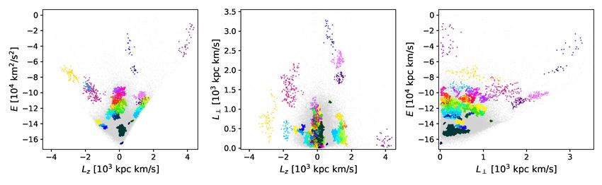
A&A proofs: manuscript no. 43060corr

     The main goal in the identification of these substructures is     real data sets. Furthermore, the vast majority of clustering algo-
to determine and characterise the merger history of the Milky          rithms require a selection of parameters that have a deterministic
Way. The identification of the various events allows placing con-      impact on the results (see e.g. Rodriguez et al. 2019, and refer-
straints on the number of accreted galaxies, their time of accre-      ences therein). At the same time, it is very difficult to physically
tion, and their internal characteristics, such as their star forma-    motivate the choice of some parameters for a given data set.
tion and chemical evolution history, their mass and luminosity,            We present a data-driven algorithm for clustering in
and the presence of associated globular clusters (e.g. Myeong          integrals-of-motion space, relying on a minimal set of assump-
et al. 2018b; Massari et al. 2019). The characterisation of the        tions. We also derive the statistical significance of each of the
building blocks is interesting from the perspective of cosmol-         structures we identified, and define a measure of closeness be-
ogy and galaxy formation because it allows the determination of        tween each star in our data set and any of the substructures. Our
the luminosity function across cosmic time, for example. Fur-          paper is structured as follows: Section 2 describes the construc-
thermore, the star formation histories and chemical abundance          tion of our data set and the quality cuts we impose, while Sec-
patterns in accreted objects permit distinguishing types of en-        tion 3 covers the technical details of the clustering algorithm.
richment sites or channels (e.g. super- or hypernovae), as well        In Section 4 we evaluate the statistical significance of the clus-
as the initial mass function in different environments. Impor-         ters we found and present some of their properties, including
tantly, many of the high-redshift analogues of the accreted galax-     their structure in velocity space. For each star in our data set, we
ies will not be directly observable in situ because of their intrin-   also provide a quantitative estimate that it belongs to any of the
sically faint luminosity, even with the James Webb Space Tele-         statistically significant clusters. The results are interpreted and
scope (JWST), and access to this population will therefore likely      discussed in Section 5. We also explore here possible relations
only remain available in the foreseeable future through studies of     between the various extracted clusters and make a comparison
nearby ancient stars. The ambitious goals of Galactic archaeol-        to previous work. The first conclusions of our study are sum-
ogy require that we are able to identify substructures in a statis-    marised in Section 6. Since our analysis is based on dynamical
tically robust way to ultimately be able to assess incompleteness      information alone, this does not fully reveal the origin of the
or biases, and to establish which stars are likely members of the      identified clusters by itself (e.g. accreted vs. in situ, see Jean-
various objects identified as this is necessary for their character-   Baptiste et al. 2017, or their relation, see Koppelman et al. 2020).
isation (eventually through detailed spectroscopic follow-up).         We devote paper II (Ruiz-Lara et al. 2022) to the characterisation
     Theoretical models and numerical simulations have shown           and nature of the structures identified in this work.
that accreted objects will preserve their coherent orbital configu-
ration long after the structure is completely phase mixed (Helmi
& de Zeeuw 2000), even in the fully hierarchical regime of the         2. Data
cosmological assembly process (Gómez et al. 2013; Simpson              The basis of this work is the Gaia EDR3 RVS sample, that
et al. 2019). One of the best ways to trace accretion events is        is, stars whose line-of-sight velocities were measured with the
to observe clustering in the integrals of motion describing the        radial velocity spectrometer (RVS) included in the Gaia Early
orbits of the stars. In an axisymmetric time-independent poten-        Data Release 3 (EDR3, Gaia Collaboration et al. 2021), sup-
tial, frequently used integrals of motion are the energy E and         plemented with radial velocities from ground-based spectro-
angular momentum in the z-direction
                             q           Lz . The component of the     scopic surveys. In particular, we extend the Gaia RVS sample
angular momentum L⊥ (= L2x + Ly2 ) is often used as well be-           with data from the sixth data release of the Large Sky Area
                                                                       Multi-Object Fiber Spectroscopic Telescope (LAMOST DR6)
cause stars originating in the same merger event are expected to
                                                                       low-resolution (Wang et al. 2020) and medium-resolution (Liu
remain clustered in this quantity as well, even though it is not
                                                                       et al. 2019) surveys, the sixth data release of the RAdial Ve-
being fully conserved (see e.g. Helmi et al. 1999). Similarly, ac-
                                                                       locity Experiment (RAVE DR6) (Steinmetz et al. 2020b,a), the
tion space can be used (see e.g. Myeong et al. 2018b), with the
                                                                       third data release of the Galactic Archaeology with HERMES
advantage that actions are adiabatic invariants, and they are less
                                                                       (GALAH DR3) (Buder et al. 2021), and the 16th data realease
dependent on distance selections (Lane et al. 2022). The actions
                                                                       of the Apache Point Observatory Galactic Evolution Experi-
have the drawback, however, that they are more difficult to de-
                                                                       ment (APOGEE DR16) (Ahumada et al. 2020). We performed
termine for a generic Galactic potential (except in approximate
                                                                       spatial cross-matching between these survey catalogues using
form, see e.g. Binney & McMillan 2016; Vasiliev 2019).
                                                                       the TOPCAT/STILTS (Taylor 2005, 2006) tskymatch2 function.
     Establishing the statistical significance of clumps identified    We allowed a matching radius between sky coordinates up to
by clustering algorithms in these subspaces is not trivial. Thus       5 arcsec after transforming J2016.0 Gaia coordinates to J2000.0,
far, many works have used either manual selection (e.g. Naidu          although the average distance between matches is ∼0.15 arcsec,
et al. 2020) or clustering algorithms in integrals-of-motion space     and 95% are below 0.3 arcsec. For the LAMOST low-resolution
successfully to identify stellar streams in the Milky Way halo         survey, we applied a +7.9 km/s offset to the measured veloc-
(Koppelman et al. 2019a; Borsato et al. 2020). In recent years,        ities according to the LAMOST DR6 documentation release1 .
works using more advanced machine learning to find clusters            Following Koppelman et al. (2019b), and based on the accu-
have also been published (Yuan et al. 2018; Myeong et al. 2018a;       racy of their line-of-sight velocity measurements, we first con-
Borsato et al. 2020). In the case of manual selection, mathemati-      sidered GALAH, then APOGEE, then RAVE, and finally LAM-
cally establishing the validity is difficult and often bypassed. For   OST while extending the RVS sample. We also imposed a max-
machine learning and advanced clustering algorithms, the results       imum line-of-sight velocity uncertainty of 20 km/s. This max-
are generally hard to interpret, especially in the case of unsuper-    imum radial velocity error introduces a small bias against very
vised machine learning, where there are no ground-truth labels.        metal-poor stars in the LAMOST-LRS data set. The final ex-
Although training and testing is possible via the use of numeri-       tended catalogue contains line-of-sight velocities for 10,629,454
cal simulations (see Sanderson et al. 2020; Ostdiek et al. 2020),      stars with parallax_over_error > 5.
these simulations have many limitations themselves, and there
                                                                       1
is no guarantee that the results obtained can be extrapolated to           http://dr6.lamost.org/v2/doc/release-note

Article number, page 2 of 16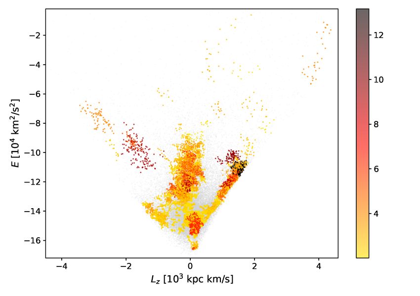
S. S. Lövdal et al.: Clustering in integrals-of-motion space

    We consider the local halo as stars located within 2.5 kpc,          important as we are dealing with unsupervised machine learn-
where the distance was computed by inverting the parallaxes              ing, therefore there is no ground truth to verify our findings with
after correcting for a zero-point offset of 0.017 mas. We re-            from a computational point of view.
quire high-quality parallaxes according to the criterion above               Our clustering algorithm will have to deal with a potentially
and low renormalised unit weight error (ruwe < 1.4). We as-              large amount of noise in search for significant clusters, which
sumed VLSR = 232 km/s, a distance of 8.2 kpc between the Sun             rules out clustering algorithms that assume that all data points
and the Galactic centre (McMillan 2017), and used (U , V , W )           belong to a cluster. Some options that can handle noise, and
= (11.1, 12.24, 7.25) km/s for the peculiar motion of the Sun            which have also been used to extract clusters in integrals-of-
(Schönrich et al. 2010).                                                 motion space, would be the friends-of-friends algorithm (Efs-
    We identified halo stars by demanding |V − VLSR | > 210              tathiou et al. 1988), used for instance in Helmi & de Zeeuw
km/s, similarly to Koppelman et al. (2018, 2019b). This cut is           (2000), DBSCAN (Ester et al. 1996), used by Borsato et al. (2020),
not too conservative and allows for some contamination from              and HDBSCAN (Campello et al. 2013), as in Koppelman et al.
the thick disk. Additionally, we removed a small number of stars         (2019a). The main problem with the first two is that they re-
whose total energy computed using the Galactic gravitational po-         quire specifying some static parameters, for example a distance
tential described in the next section is positive. The resulting data    threshold for data points of the same cluster. As there is a gradi-
set contains N = 51671 sources, and we refer to this selection as        ent in density in our halo set (especially, fewer stars with lower
the halo set.                                                            binding energies), using static parameters for this will only work
    The relative parallax uncertainty of the stars in this               well on some parts of the data space, unless we first apply some
halo sample is lower than 20%. For example, the median                   advanced non-linear transformations. HDBSCAN is able to extract
parallax_error/parallax for the Gaia RVS sample is ∼                     variable density clusters, but in addition to having a slight black-
2.4%, while for the full extended sample (Gaia RVS plus                  box tendency in the application, the output is also dependent on
ground-based spectroscopic surveys), it is ∼ 3.7%. The radial ve-        some user-specified parameters. We wish to make as few as-
locities of the stars from the Gaia RVS sample have much lower           sumptions as possible about the properties of the clusters and
uncertainties than the cut of 20 km/s, with a median line-of-sight       also desire full control over the clustering process, therefore we
velocity uncertainty of 1 km/s. The full extended (halo) sam-            consider a simpler option.
ple has a median line-of-sight velocity uncertainty of 6.7 km/s,             The single-linkage algorithm is a hierarchical clustering
driven mostly by the higher uncertainties associated with the            method that only requires a selection of distance metric (Everitt
LAMOST DR6 low-resolution radial velocities. These uncer-                et al. 2011). We used standard Euclidean distance to this end.
tainties (as well as those in the proper motions) drive the un-          At each step of the algorithm, it connects the two groups with
certainties in the total velocities of the stars in our halo sample,     the smallest distance between each other, defined as the small-
as well as in their integrals of motion (see Sec. 3.2). The me-          est distance between two data points not yet in the same group,
dian uncertainty in the total velocity, v, is 4.1 km/s for stars from    where each data point is considered a singleton group initially.
the Gaia RVS sample and 9.1 km/s for those from the extended             Each merge, or step i of the algorithm, corresponds to a new
sample.                                                                  connected component in the data set. This is illustrated in Fig. 1.
                                                                         Here single-linkage is applied on a two-dimensional example,
                                                                         where the top part of each panel illustrates the merging process
3. Methods                                                               of the algorithm, and in the bottom we illustrate the resulting
                                                                         merging hierarchy in a dendrogram. If the data set is of size
One of the primary goals of this work is to develop a data-driven        N, the algorithm performs N − 1 steps in total as it continues
algorithm, where the extracted structures are statistically based        until the full data set has been linked. Hence, the algorithm is
and easily interpretable. At the same time, we desire a method           also closely related to graph theory, as the result after the last
that detects more than the most obvious clusters, but that is ide-       merge is equivalent to the minimum spanning tree (Gower &
ally able to scan through the data set without missing any signal.       Ross 1969). From a computational point of view, the series of
    In what follows, we use the following notation: x for a data         connected components that is obtained also corresponds to the
point, or star, in our clustering space. The dimensionality of our       set of every potential cluster in the data, under the assumption
data space is denoted by n, N is the number of stars in the data         that the most likely clusters are the groups of data points with
set after applying quality cuts, and as described in Sec. 2, we          the smallest distance between each other, without assuming any
call this selection the halo set. Ci denotes a connected compo-          specific cluster shape.
nent in the halo set, having been formed at step i of the cluster-           The core idea of our clustering method is to apply the single-
ing algorithm. Each Ci is a candidate cluster for which we wish          linkage algorithm to the halo set and subsequently evaluate each
to evaluate the statistical significance. We denote the number of        connected component (or candidate cluster Ci , formed at step i
members of a candidate cluster NCi .                                     of the algorithm) by a cluster quality criterion. The clusters that
    We consider the data points as such, without taking measure-         exhibit statistical significance according to the selected criterion
ment uncertainties into account. While this would technically be         are accepted. In this way, the method is also able to handle noise
possible, the quality cuts we impose on the data are strict enough       because the data points that do not belong to any cluster display-
to result in reasonably robust outcomes, and we leave it to future       ing a high statistical significance are discarded.
work to extend the method by taking uncertainties into account
in a probabilistic way.
                                                                         3.2. Clustering in integrals-of-motion space

3.1. Clustering algorithm: Single-linkage                                As described earlier, to identify merger debris, we relied on the
                                                                         expectation that it should be clustered in integrals-of-motion
A range of clustering algorithms is available, but we desire max-        space. As integrals of motion, we used three typical quanti-
imum control over the process, in combination with an exhaus-            ties: The angular momentum in z-direction Lz , the perpendicular
tive extraction of information in the data set. This is especially       component of the total angular momentum vector L⊥ , and total
                                                                                                                 Article number, page 3 of 16
A&A proofs: manuscript no. 43060corr
5 1 5 1 5 1 5 1 5 1
2 2 2 2 2
4 4 4 4 4
3 3 3 3 3
6 6 6 6 6
7 7 7 7 7
8 8 8 8 8
1 2 3 4 5 6 7 8 1 2 3 4 5 6 7 8 1 2 3 4 5 6 7 8 1 2 3 4 5 6 7 8 1 2 3 4 5 6 7 8
Fig. 1. Single linkage algorithm applied on a two-dimensional example. Each step of the algorithm forms a new group by connecting the two
closest data points not yet in the same cluster, where each data point is considered a singleton group initially. The resulting merging hierarchy is
visualised as a dendrogram at the bottom of each panel.
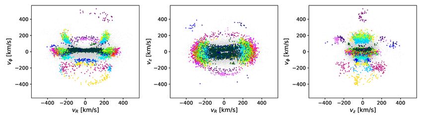
Fig. 2. Distribution of stars in our halo sample in integrals-of-motion space. The single-linkage algorithm identifies clusters in the three-
dimensional space resulting from the combination of our three clustering features, namely energy E, and two components of the angular momentum
Lz and L⊥ .
energy E. While Lz is truly conserved in an axisymmetric po- and maximum values in the halo set. Our equal-range scaling
tential, L⊥ typically varies slowly, retaining a certain amount of also implies that each of the three features is considered equally
clustering for stars on similar orbits as those originating in the important in a distance-based clustering algorithm. The typi-
same accretion event, although not being fully conserved. The cal (median) errors in these quantities are much smaller than
total energy E is computed as the range they cover. In the full halo sample, for example, for
the energy hσE i ∼ 1052 km2 /s2 ; and for the angular momenta
1 2 hσLz i ∼ 61 kpc km/s and hσL⊥ i ∼ 46 kpc km/s, , while for the
E= v + Φ(r), (1)
2 subset with Gaia RVS velocities, the typical uncertainties are a
factor 2.5 – 3.5 smaller. The halo set visualised for all combina-
where Φ(r) is the Galactic gravitational potential at the location tions of the clustering features is shown in Fig. 2.
of the star. For this we used the same potential as in Koppelman
et al. (2019b): A Miyamoto-Nagai disk, Hernquist bulge, and
Navarro-Frank-White halo with parameters (ad , bd ) = (6.5, 0.26) 3.3. Random data sets
kpc, Md = 9.3 × 10¹⁰ M for the disk, cb = 0.7 kpc, Mb =
3.0 × 10¹⁰ M for the bulge, and r s = 21.5 kpc, ch =12, and To assess the statistical significance of the outcome of our clus-
Mhalo = 1012 M for the halo. While the choice of potential in- tering algorithm, we used random data sets. To this end, we
fluences the absolute values we computed for total energy, the created a reference halo set using our existing data set, but re-
difference in the distributions of data points between two rea- computed the integrals of motion using random permutations of
sonably realistic potentials is negligible in the clustering space, the vy and vz components, similarly to Helmi et al. (2017). This
as shown in Section 5. created an artificial data set with similar properties to the ob-
We scaled each of the integrals of motion, or ‘features’, served data, but where the correlations in the velocity compo-
linearly to the range [−1, 1] using a set reference range of nents and hence structure in integrals of motion space is broken
E = [−170000, 0] km2 /s2 , L⊥ = [0, 4300] kpc km/s, and Lz = up. Specifically, we scrambled the velocity components of all
[−4500, 4600] kpc km/s, roughly corresponding to the minimum stars with |V − VLSR | > 180 km/s (a slightly more relaxed defi-
Article number, page 4 of 16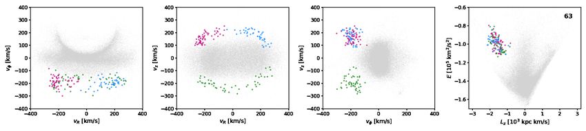
S. S. Lövdal et al.: Clustering in integrals-of-motion space

Fig. 3. Example of the distribution of points in integrals of motion for one of the random halo sets (number 1 out of Nart = 100) obtained by
re-shuffling the velocity components. See for comparison Fig. 2.

nition of the halo, comprising 75149 sources of our original data        equation of an n-dimensional ellipsoid centred around the origin
set). The majority of these stars with scrambled velocities sat-         is
isfied the criterion we used to kinematically define halo stars,         X n
                                                                              xi2
|V − VLSR | > 210 km/s. For each artificial halo, we therefore                    = 1,                                                (2)
sampled N stars satisfying the above-mentioned criterion and                 a2
                                                                          i=1 i
recomputed the clustering features, where N is the number of             where ai denotes the length of each axis. The variance along each
stars in our original halo set. We normalised these features with        principal component of the cluster is given by the eigenvalues λi
the same scaling as for the original halo set, such that the map-        of the covariance matrix, and we can define the length of each
ping from absolute to scaled values was identical for the real and       axis ai of the ellipsoid in terms of the number of standard de-
artificial data.                                                         viations of spread along the corresponding axis. We consulted
     We generated Nart = 100 realisations of this artificial halo as     the χ2 distribution with three degrees of freedom (correspond-
reference. An example artificial data set is displayed in Fig. 3,        ing to our three-dimensional clustering space) and observed that
where an arbitrarily chosen realisation is visualised. By compar-        95.4% of a three-dimensional Gaussian distribution falls within
ing to Fig. 2, we see that the two data sets have very similar char-     2.83 standard deviations of extent along each axis. This is the
acteristics, but that the substructure visible by eye in the original    fraction of a distribution that directly corresponds to the length
halo set has been diluted.                                               of two standard deviation axes in a univariate   √         space. Hence, we
                                                                         chose the axis lengths to be ai = 2.83 λi . The choice to cover
                                                                         95.4% of the distribution provides a snug boundary around the
4. Results                                                               data points that is neither too strict nor includes too much empty
4.1. Identification of clusters                                          space.
                                                                              We then computed the number of stars falling within the el-
We applied the algorithm described above on our halo set. We             lipsoidal cluster boundary by analysing the PCA transformation
only investigated candidate clusters with at least ten members,          of Ci and mapping the stars of the data sets to the PCA space de-
evaluating them according to the procedure described in the next         fined by Ci by subtracting the means and multiplying each data
section, as this is the smallest group that would be statistically       point by the eigenvectors of the covariance matrix. Hereby we
significant assuming Poissonian statistics together with the sig-        obtained a mean centred and rotated version of the data in which
nificance level we adopted.                                              the direction of maximum variance aligns with the axis of the
                                                                         coordinate system.
4.1.1. Evaluating statistical significance                                    We computed both the average number of stars from the ar-
                                                                         tificial halo hNCarti i and the number of stars from the real halo set
In order to examine the quality of each candidate cluster obtained       NCi that fall within this boundary. The statistical significance of a
by the linking process, we need a cluster evaluation metric. A           cluster was then obtained by the difference between the observed
challenge is that our three-dimensional clustering space has a           and expected count, divided by the statistical error on both quan-
higher density of stars with low energy and angular momentum             tities. We required a minimum significance level of 3σ, defined
than regions with higher energy, as shown in Fig. 2. Therefore we        by
used our randomised data sets to compare the observed and ex-
pected density for different regions. We thus examined the can-          NCi − hNCarti i > 3σi ,                                                  (3)
didate clusters resulting from applying the single-linkage algo-
                                                                                                 q
                                                                         and where σi =            NCi + (σCarti )2 . Here σCarti is the standard de-
rithm and assessed their statistical significance by computing the
expected density of stars in a region, and comparing the differ-         viation in the number counts across our 100 artificial halos. We
ence between the observed and expected count in relation to the          treated the observed data as having Poissonian properties,       p giving
statistical error on these quantities.                                   the statistical error on the observed cluster count as NCi .
    In order to compare the number of members of a candidate
cluster Ci to the expected count (obtained from our randomised           4.1.2. Statistically significant groups
sets), we determined the region in which Ci resides. To this end,
we defined an ellipsoidal boundary around Ci by applying prin-           Evaluating the statistical significance for all candidate clusters
cipal component analysis (PCA) on the members. The standard              returned by the single linkage algorithm returned a set of clus-
                                                                                                                      Article number, page 5 of 16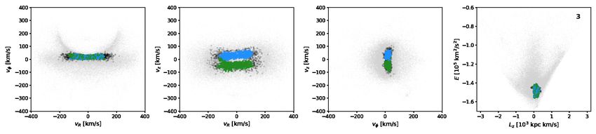
A&A proofs: manuscript no. 43060corr

Fig. 4. Clusters extracted by the algorithm, visualised in integrals of motion (top row) and in velocity space (bottom row). The different colours
indicate the stars associated with the 67 different clusters we identified.

ters with a 3σ significance at least, some of which were hierar-
chically overlapping subsets of each other. A structure is likely to
display statistical significance starting from the core of the clus-
ter, growing out to its full extent via a series of merges in the al-
gorithm, each being deemed statistically significant. Similarly, a
cluster with a dense core together with some neighbouring noise
still displays significance if the core is dense enough.
     Under the hypothesis that the statistical significance in-
creases while more stars of the same structure are being merged
into the cluster and that the significance decreases when noise
in the outskirts is added, final (exclusive) cluster labels were
found by traversing the merging tree of the overlapping signif-
icant clusters and selecting the location at which they reached
their maximum significance. In practice, this was done by iterat-
ing over the clusters ordered by descending significance, travers-
ing its parent clusters upwards in the tree, and selecting the
location where the maximum significance was reached. Nodes
higher up in the merging hierarchy than the maximum signifi-
cance for this path were removed because we did not aim for a             Fig. 5. Distribution of the 67 high-significance clusters in the E − Lz
path with a smaller maximum significance to override the selec-           plane, colour-coded according to their statistical significance as com-
tion by deeming a larger cluster on the same path to be a final           puted by Eq. 3.
cluster.
     After finding a cluster in the tree at its maximum signifi-          space (bottom panel). The colours here are for illustration pur-
cance, we assigned the same label to all stars that belonged to           poses only, and there are enough clusters such that some of them
this connected component according to the single linkage algo-            are plotted in very similar shades.
rithm. Conveniently, if we were to chose a lower significance                 One of clusters identified by the single-linkage algorithm
level than 3σ, the change would simply extract additional clus-           (assigned label, or cluster ID 1) is the globular cluster M4.
ters of a lower significance that do not overlap with those of            This cluster has the lowest energy and is shown in dark blue
higher significance.                                                      in the top left panel of Fig. 4. Although all of its associ-
     The results of the methodology described above are shown             ated stars have nominally good parallax estimates, a subset
in Fig. 4, which plots the distribution of the individual clusters        has rather high correlation values in the covariance matrix
identified for the various subspaces (top panel) and in velocity          provided by the Gaia database, particularly for terms involv-
Article number, page 6 of 16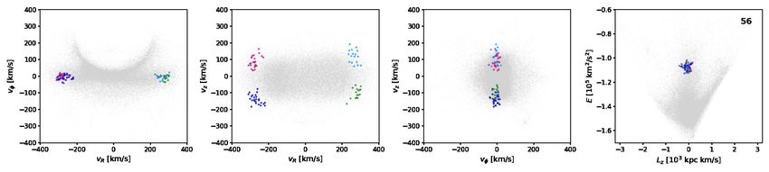
S. S. Lövdal et al.: Clustering in integrals-of-motion space

                                                                         set representing such a cluster in velocity space is far smaller
                                                                         and less complex than our original halo set, and because the sub-
                                                                         groups in velocity space are often clearly separated clumps, we
                                                                         simply applied the HDBSCAN algorithm (Campello et al. 2013)
                                                                         once for each cluster. This is a robust clustering algorithm that
                                                                         can extract variable density clusters and labels possible noise,
                                                                         while being able to handle various cluster shapes.
                                                                              We applied HBDSCAN directly to the vR , vφ , and vz compo-
                                                                         nents of each cluster without scaling because the range for these
                                                                         values is already of the same magnitude. We set the parame-
                                                                         ter min_cluster_size (smallest group of data points that the
                                                                         algorithm accepts as an entity) to 5% of the cluster size, with
                                                                         a lower limit of three stars. We assigned min_samples = 1,
                                                                         which regulates how likely the algorithm is to classify an out-
                                                                         lier as noise, with a lower value being less strict. The default
                                                                         mode of HDBSCAN does not allow for a single cluster to be
Fig. 6. Histogram of the number of members per cluster. Members          returned, as its excess of mass algorithm may bias towards the
identified by the single-linkage algorithm are plotted in solid blue.    root node of the data hierarchy. Because a single-linkage cluster
The dashed red line indicates the sizes when original and additional     might correspond to a single group in velocity space but this is
plausible members are considered within a Mahalanobis distance of        not always the case, we circumvented this issue by setting the
Dcut ∼ 2.13 from each cluster centre.
                                                                         parameter allow_single_cluster to True only if the stan-
                                                                         dard deviation in vR , vφ , and vz was small (below 30 km/s) for
ing the parallax (explaining finger-of-god features in velocity          at least two out of the three velocity directions. The idea is that
space). This finding prompted us to inspect all of the signif-           if a cluster seems to be a single subgroup, it might display an
icant clusters, and we realised that cluster 67 also has mem-            elongated dispersion along one of these components at most, but
bers with similarly high values of correlation terms involving           if the dispersion is large for two or more out of the three, the
parallax (namely those with declination and µδ , in particular,          cluster is likely to contain at least two kinematic subgroups.
most of its stars either have dec_parallax_corr that is be-                   In this way, the HDBSCAN algorithm extracted 232 sub-
low -0.15 or parallax_pmdec_corr above 0.15). These stars                groups, where the number of subgroups per cluster varied in
are also located towards the Galactic centre and anticentre,             the range [1, 12], with the mean and median being 3.5 and 3,
that is, they also lie in relatively crowded regions. The aver-          respectively. This is likely a lower limit to the true number of
age value of the stars in cluster 67 in dec_parallax_corr and            subgroups in velocity space, particularly because of the limita-
parallax_pmdec_corr is significantly lower than that of any              tion in the number of stars, which prevented us from detecting
other cluster, resulting in an average parallax_err=0.1, com-            streams with fewer than three stars in the data set, but also due
pared to an average value lower than 0.045 for all other clusters.       to the difficulty with defining optimal parameters for clustering
To avoid confusion, we did not plot this cluster in Figure 4 and         in this space.
did not consider it further in our analysis.                                  A series of examples of the output of HDBSCAN is dis-
     Figure 5 shows the clusters colour-coded by their statistical       played in Fig. 7. Here each row reflects one cluster; the first three
significance. The algorithm identified 67 clusters to which a to-        panels display the projection of the subgroups in velocity space,
tal of 6209 stars were assigned. The range of significance values        and the rightmost panel displays the location of the cluster in
is [3.0, 13.2]. The figure shows that the clusters with the highest      E − Lz space. The cluster ID is indicated in the top right corner.
significance are located in regions of already known substruc-           Non-members are plotted in grey, and noise as labelled by HDB-
tures, such as the Helmi Streams near Lz ∼ 1500 kpc km/s and             SCAN is shown with open black circles. The subgroups in veloc-
E ∼ −105 km2 /s2 (Helmi et al. 1999; Koppelman et al. 2019b).            ity space for the statistically significant clusters are often quite
     In Fig. 6 we show the distribution of the number of members         distinct, for example in the case of clusters 3, 4, and 56. Cluster
of the clusters identified by our procedure, plotted as the his-         3 is an example of a cluster that would be classified as a single
togram with blue bars. The median number of stars in a cluster is        subgroup if the parameter allow_single_cluster were stati-
53, and 2137 stars are associated with the largest cluster. These        cally True, demonstrating the necessity of our approach. Cluster
numbers reflect the members identified by the linking process,           63 is split into three subgroups, even though it could possibly be
which belong to some significant cluster Ci . For most clusters,         divided into either two or four groups as well. Cluster 64 has the
it is possible to identify additional plausible members following        largest number of subgroups; it is divided into 12 small portions.
the procedure described in Sec. 4.3. The resulting cluster sizes              The dispersion in the velocity components of these sub-
are shown as the dashed red histogram in Fig. 6.                         groups can be used to characterise them further. This was com-
                                                                         puted by applying PCA on the v x , vy , and vz components of each
4.2. Extracting subgroups in velocity space                              subgroup with at least ten members (107 in total), and measur-
                                                                         ing the standard deviation along the resulting principal compo-
The velocity distributions of the extracted clusters contain more        nents. A histogram of these dispersions is displayed in Fig. 8.
clues about their validity and properties because an accreted            In 11 subgroups, the dispersion in the third principal component
structure observed within a local volume is expected to display          is smaller than 10 km/s, and in 3 subgroups, it is below 5 km/s.
(sub)clumping in velocity space. This represents debris streams          The lowest value of 2.5 km/s is associated with the globular clus-
with different orbital phases.                                           ter M4 (cluster 1) and the second smallest (4.4 km/s) with cluster
    We extracted these subgroups in velocity space by applying           64, which is shown as the yellow subgroup in the corresponding
another round of clustering on each of the 67 clusters. As the data      panel in Figure 7.
                                                                                                                  Article number, page 7 of 16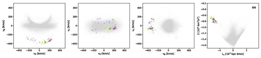
A&A proofs: manuscript no. 43060corr

Fig. 7. Subgroups identified by HDBSCAN in velocity space for a selection of five significant clusters from the single-linkage algorithm, where
noise as labelled by the algorithm is marked with open black circles. In each row, the three first panels display the projection of the subgroups in
velocity space, and the fourth panel shows the location of the ‘parent’ cluster in E − Lz space; its ID is displayed in the upper right corner.

    The distribution of the three-dimensional velocity dispersion          4.3. Evaluating the proximity of stars to clusters
σtot of the subgroups is shown in the bottom panel in Fig. 8,
where the lowest value is again obtained for the globular clus-            Now that we have obtained our cluster catalogue, we would like
ter M4. A single subgroup, the green subgroup of cluster 63 in             to obtain estimates for the likelihood of any individual star to
Fig. 7, is truncated from Fig. 8 as it has a total velocity dispersion     belong to some specific cluster. This was done both in order to
of 186 km/s.                                                               identify possible new members of a cluster and to find the most
                                                                           likely members for observational follow-up, for instance.
                                                                               To do this, we described each cluster in integrals-of-motion
                                                                           space as a Gaussian probability density, defined by the mean and
                                                                           covariance matrix of the associated stars identified by the single-
                                                                           linkage algorithm. The idea is that the core of the overdensity is
Article number, page 8 of 16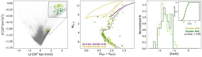
S. S. Lövdal et al.: Clustering in integrals-of-motion space

                                                                         Fig. 9. Distribution of squared Mahalanobis distances of the stars as-
                                                                         signed to a cluster vs. the chi-square distribution with three degrees of
                                                                         freedom.

                                                                         Fig. 9). Specifically, we checked the distribution of stars in the
                                                                         colour-absolute magnitude diagrams and the metallicity distribu-
                                                                         tion functions for each cluster. A too restrictive cut (50th, 65th
                                                                         percentiles) reduces the number of stars in a way that often lim-
                                                                         its the characterisation of the cluster properties. A too loose cut
                                                                         (95th, 99th percentiles), although greatly increasing the number
                                                                         of stars in clusters, leads to a noticeable amount of contamina-
                                                                         tion, hence affecting the cluster properties. As a compromise be-
                                                                         tween a manageable amount of contamination and an increase in
Fig. 8. Velocity dispersions of each subgroup with at least ten mem-     purity of the clusters as well as in the number of stars, we decided
bers identified by HDBSCAN, computed along the principal axes of the     to use the 80th percentile cut, corresponding to a Mahalanobis
Cartesian velocity components (top three panels), and the total three-   distance of Dcut ∼ 2.13.
dimensional value (bottom panel).                                             Out of the stars in our halo set that did not yet receive a label,
                                                                         we can associate 2104 additional stars with one of the clusters on
                                                                         the basis of the star being within a Mahalanobis distance of 2.13
located around the mean of the Gaussian, and less likely mem-
                                                                         to its closest cluster. There are 1186 original members falling
bers are located in the outskirts of the distribution. We then com-
                                                                         outside of the Mahalanobis distance cut. In total, 7127 stars in
puted the location of a data point x within the Gaussian distribu-
                                                                         the halo set (13.8%) lie within Dcut = 2.13 of some cluster.
tion by calculating its Mahalanobis distance D,
                                                                              The histogram of the number of cluster members contained
      q                                                                  within Dcut is displayed in Fig. 6 as the dashed red line. The
D = (x − µ)T Σ−1 (x − µ),                                        (4)     largest cluster, cluster 3, has 3032 such members, while the
                                                                         smallest cluster is cluster 34, with 9 such members. The mean
where µ is the mean of the cluster distribution and Σ−1 is the in-       and median sizes of the clusters after the identification of addi-
verse of the covariance matrix. Therefore, the Mahalanobis dis-          tional members within Dcut become 106 and 49, respectively.
tance expresses the distance between a data point and a Gaussian              Table 1 lists the clusters we identified, their statistical signif-
distribution in terms of standard deviations after that the distri-      icance (σi ), the number of members indicated by the clustering
bution has been normalised to unit spherical covariance.                 (Norig ) and with additional members (Ntot ), the centroid (µ), and
    The theoretical distribution of squared Mahalanobis dis-             entries of covariance matrix (σi j ). To transform the values listed
tances of an n-dimensional Gaussian is known: it is the χ2 distri-       in the table into the corresponding physical quantities, we can
bution with n degrees of freedom. Fig. 9 shows the distribution          use for the means that
of Mahalanobis distances for the stars assigned to clusters by our
procedure, compared to the χ2 with n = 3 degrees of freedom.                       2
                                                                         hµi i =      (hIi i − Ii,min ) − 1,
This figure demonstrates that the distribution of the members of                   ∆i
the clusters is somewhat similar to a multivariate Gaussian, but
                                                                         where ∆i = Ii,max − Ii,min , with i = 0..2 and Ii corresponding to
that this is slightly more peaked in comparison to what is seen
                                                                         E, L⊥ , and Lz , with the minimum and maximum values given in
for the cluster members.
                                                                         Sec. 3.2. For the covariance matrix, these definitions lead to
    We can therefore use the Mahalanobis distance of each star
to refine the detected clusters, select core members, and identify                  4
additional plausible members. To establish a meaningful value            σi j =          ΣI
                                                                                   ∆i ∆ j i, j,
of the Mahalanobis distance Dcut , we proceeded as follows. We
investigated the internal properties of the clusters as defined by       where ΣIi, j is the covariance matrix in integrals-of-motion space.
the algorithm and by considering only the stars within different         Table 2 lists the kinematic and dynamical properties for the stars,
values of Dcut (corresponding to the 50th, 65th, 80th, 90th, 95th,       as well as the cluster with which they were associated by the
and 99th percentiles of the distribution of original members, see        single-linkage algorithm and that with which they are associated
                                                                                                                    Article number, page 9 of 16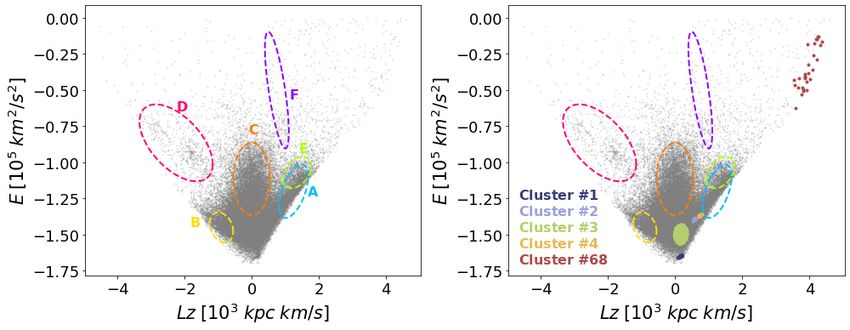
A&A proofs: manuscript no. 43060corr

on the basis of their Mahalanobis distance, which is also listed      the finer structures within the groups would require a detailed
to help assess membership probability. Both tables are available      analysis of the internal properties of these clusters and substruc-
online in their entirety.                                             tures, such as their stellar populations, metallicities, and chemi-
                                                                      cal abundances. We defer such an exhaustive analysis to a sepa-
                                                                      rate paper (Ruiz-Lara et al. 2022). Nonetheless, as a first exam-
5. Discussion                                                         ple, we here focus our attention on the pair of clusters 60 and 61,
The relatively large number of clusters we identified means that      identified as substructure E, which are likely part of the Helmi
it is important to understand how they relate to each other. We       streams (Helmi et al. 1999).
explored their internal hierarchy in our clustering space using the        These two clusters are directly linked according to the den-
Mahalanobis distance between two distributions,                       drogram in Fig. 10. The middle and right panels of Fig. 12 show
       q                                                              the colour absolute magnitude diagram (CaMD) and the metal-
D0 = (µ1 − µ2 )T (Σ1 + Σ2 )−1 (µ1 − µ2 ),                       (5)   licity distribution functions (from the LAMOST-LRS survey) for
                                                                      both clusters. In the CaMD we corrected for reddening using the
where µ1 , µ2 and Σ1 , Σ2 describe the means and covariance ma-       dust map from Lallement et al. (2018) and the recipes to trans-
trices of the two cluster distributions, respectively, and D0 gives   form into Gaia magnitudes given in Gaia Collaboration et al.
a relative measure of their degree of overlap. A dendrogram of        (2018a). These figures demonstrate that indeed, the cluster stars
the clusters according to single linkage by Mahalanobis distance      depict similar distributions in the CaMD, with ages older than
is shown in Fig. 10.                                                  ∼ 10 Gyr, and metallicities drawn from the same distribution,
                                                                      having a Kolmogorov-Smirnov statistical test p-value of 0.99.
                                                                      All this evidence supports a common origin for both clumps as
5.1. Number of independent clusters                                   debris from the Helmi streams.
An initial inspection of the dendrogram shown in Fig. 10 reveals           The separation of the Helmi streams into two significant
a complex web of relations between the significant clusters we        clusters in integrals-of-motion space agrees with the recent find-
extracted with our single-linkage algorithm. Some of these clus-      ings presented in Dodd et al. (2022). In this work, the authors
ters are linked to others only at large distances (clusters 1, 2,     established that the two clumps, which are clearly split in angu-
3, 4, or 68), whereas others are clearly grouped together, some-      lar momentum space in a similar manner as our clusters 60 and
times even in a hierarchy of substructures. This suggests that the    61, are the result of a resonance in the orbits of some of the stars
67 clusters that our methodology identified as significant are not    in the streams. This effect is thus a consequence of the Galactic
fully independent of each other. The proper assessment of the         potential. We preliminarily conclude that analyses such as those
independence of the different clusters is presented in paper II,      presented for the Helmi streams here, using the internal prop-
Ruiz-Lara et al. 2022.                                                erties of the clusters identified by our algorithm, can help us in
    As a first attempt to explore the hierarchy we observe in the     fully assessing and characterising the different building blocks
dendrogram, we tentatively set a limit at Mahalanobis distance        in the Galactic halo near the Sun.
∼ 4.0 (horizontal dashed line in Fig. 10). This Mahalanobis dis-
tance is large enough such that not all 67 clusters are consid-       5.2. Relation to previously detected substructures
ered individually (the lower limit is set by the Helmi streams,
see the discussion below and Dodd et al. 2022), but also small        Several attempts have been made to identify kinematic substruc-
enough that at least some substructures reported in the literature    tures in the Milky Way halo after the Gaia data releases. Here we
can be distinguished (see e.g. Koppelman et al. 2019a; Naidu          focus on three studies that have selected or identified multiple
et al. 2020). According to this experimental limit, we may tenta-     kinematic substructures using the data from Gaia DR2 (Koppel-
tively identify six different large substructures (colour-coded in    man et al. 2019a; Naidu et al. 2020; Yuan et al. 2020b). Fig. 13
Fig. 10), as well as a few independent clusters. The distribution     presents the comparisons in the Lz − E space. Although the three
of these substructures in the E − Lz plane, together with that of     comparison studies defined kinematic substructures using Lz and
the isolated clusters (numbers 1, 2, 3, 4, and 68), is displayed in   E and/or provided average Lz and E of the substructures, they
Fig. 11. This figure shows that some of these groups do indeed        adopted different Milky Way potentials (and a slightly different
correspond to previously identified halo substructures (see also      position and velocity for the Sun). We therefore recomputed Lz
Sec. 5.2). Interestingly, there are also some examples of clus-       and E of the stars in our study in the default Milky Way potential
ters with hot thick-disk-like kinematics, such as those associated    of the python package gala (Price-Whelan 2017), which was
with substructure A, or clusters 2 to 4.                              used in Naidu et al. (2020), and in the Milky Way potential of
    The rich substructure found by the single linkage algorithm       McMillan (2017), which was used in the other two studies. Re-
within each of these tentative groups deserves further inspection.    assuringly, Fig. 13 shows that the clusters we identified remain
For instance, the large group labelled C in Fig. 10, which accord-    tight even in these other Galactic potentials. In addition to these
ing to its location in the E − Lz plane could correspond to Gaia-     three studies, we also made a comparison with (Myeong et al.
Enceladus (Helmi et al. 2018), can be clearly split into several      2019), although we note that their identification of substructure
subgroups according to the dendrogram. In addition, there are         was made in subspaces different than in our study.
some individual clusters such as cluster 6, linked at large Ma-           Based on the data from the H3 survey (Conroy et al. 2019),
halanobis distances, that might be considered as part of Gaia-        Naidu et al. (2020) investigated the properties of a number of
Enceladus. Similarly, clusters belonging to the light blue branch     substructures by defining selection boundaries simultaneously in
(substructure B), which falls in the region in E − Lz occupied by     dynamical and in the α-Fe plane. Their sample consists of stars
Thamnos (Koppelman et al. 2019a), also show different cluster-        with a heliocentric distance larger than 3 kpc, and therefore it
ing levels. Cluster 37 is linked at a larger Mahalanobis distance     is complementary to our study, which focuses on stars within
than clusters 8 and 11.                                               2.5 kpc from the Sun. Even though the spatial coverage is dif-
    To fully assess the tentative division of our halo set into six   ferent, the agreement with our work is generally good; we find
main groups and to study the significance and independence of         significant clusters with Lz and E close to the average properties
Article number, page 10 of 16
S. S. Lövdal et al.: Clustering in integrals-of-motion space
Table 1. Overview of the characteristics of the extracted clusters. We list their significance, the number of members as determined by the single-
linkage (Norig ) and in total after considering members within a Mahalanobis distance of 2.13 (NDcut ). µ is the centroid of the scaled clustering
features as determined by the original members, and σi j represents the corresponding entries in the covariance matrix. The indices 0-2 correspond
to the order E, L⊥ , and Lz . The full table is made available online.
Label signif. Norig NDcut µ0 [10−3 ] µ1 [10−3 ] µ2 [10−3 ]
1 6.0 42 33 -941.5 -989 22
2 3.1 15 12 -640.1 -952 114
3 6.3 2137 3032 -759.6 -851 24
4 3.3 18 14 -607.4 -450 152
5 4.1 69 65 -519.7 -703 -38
6 3.0 118 122 -546.2 -809 -47
7 3.8 88 91 -533.0 -914 -60
8 3.1 60 70 -699.6 -757 -201
9 3.1 29 17 -488.2 -659 -51
10 3.1 48 58 -505.8 -869 -83
σ00 [10−6 ] σ01 [10 ]
−6
σ02 [10 ]
−6
σ11 [10−6 ] σ12 [10−6 ] σ22 [10−6 ]
50.7 6.3 52.7 21.0 9.2 76.9
57.6 37.8 30.7 28.5 19.1 25.8
1324.0 255.9 23.2 3916.6 210.6 369.2
42.9 -11.3 44.0 49.1 -19.2 81.3
276.8 157.7 -63.5 221.7 -63.7 179.5
433.2 -252.2 102.0 484.5 -133.5 311.3
136.6 -49.0 -51.0 410.1 231.0 418.6
179.0 -139.4 -79.4 484.1 168.0 296.1
63.4 24.2 -37.9 160.9 -76.5 214.2
648.9 31.8 216.3 241.8 -65.5 162.4
Fig. 10. Relation between the significant clusters according to the single-linkage algorithm, obtained using the Mahalanobis distance in clustering
space.
of some structures from Naidu et al. (2020). However, we also prominent at larger distances than 2.5 kpc from the Sun (the dis-
find some differences for Aleph, Wukong, Thamnos, and Arjuna, tance limit of our sample). It therefore remains to be seen if the
Sequoia, and I’itoi. algorithm presented in this work confirms the existence of LMS-
In particular, we do not find significant clusters that would 1/Wukong when it is applied to a sample that covers a larger vol-
correspond to their Aleph and Wukong. Although several clus- ume. We note, however, that clusters with 2σ significance exist
ters (clusters 12, 27, 39, 52, and 54) have some stars in the in the region of Wukong according to our single-linkage algo-
Wukong selection box, they are located at the edge. We do not rithm (see Figure 14).
find any clusters that have similar values of Lz and E as the av- We also find some differences when we compare the distri-
erage values of Wukong stars from Naidu et al. (2020). The ab- bution of our significant clusters with Thamnos and Arjuna, Se-
sence of Aleph in our data is likely due to our |V − VLSR | > quoia, and I’itoi as defined by Naidu et al. (2020). Our analy-
210 km/s selection of halo stars, which would remove essentially sis has identified a group of clusters with retrograde motion and
all the stars on Aleph-like orbits. On the other hand, the reason with low-E that is clearly separated from Gaia-Enceladus, which
for the absence of Wukong is less clear. would likely correspond to Thamnos according to the definition
Independently of Naidu et al. (2020), Yuan et al. (2020a) of Koppelman et al. (2019a), as discussed in the next paragraph.
identified a stellar stream called LMS-1 from the analysis of On the other hand, the average Lz and E of Thamnos by Naidu
K giants from LAMOST DR6, which they associated with et al. (2020) are clearly different, occupying the region where
two globular clusters that Naidu et al. (2020) associated with we would probably associate clusters with Gaia-Enceladus, as
Wukong. Because the findings by Yuan et al. (2020a) are based shown in the top panel of Fig. 13. In the region occupied by Ar-
on stars with heliocentric distance of ∼ 20 kpc and because stars juna, Sequoia, and I’itoi, which according to Naidu et al. (2020)
in Naidu et al. (2020) are also more distant than our sample, contains three distinct structures with similar average kinematic
we may tentatively conclude that LMS-1/Wukong might be only properties but different characteristic metallicities, we also find
Article number, page 11 of 16A&A proofs: manuscript no. 43060corr
Table 2. Overview of fields in our final star catalogue. It contains Gaia source ids, heliocentric Cartesian coordinates, heliocentric Cartesian
velocities, and the three features we used for clustering. The column significance indicates the significance of the cluster to which a star belongs
(according to the original single-linkage assignment), Labelorig is the label of the cluster according to the single-linkage process, and LabelDcut is
the cluster label after selecting the cluster with the smallest Mahalanobis distance D (requiring at least D < 2.13). The full table is made available
online.
source_id x y z vx vy vz
[km/s] [km/s] [km/s]
494990686553088 -0.82 0.07 -0.92 -252.3 -249.5 29.7
2131751183780736 -0.52 0.07 -0.54 -262.9 -247.3 45.4
2412092288843648 -0.12 0.01 -0.12 -105.8 -210.9 -51.9
4032119593003520 -1.56 0.17 -1.49 220.9 -239.3 72.0
4564455019620096 -0.58 0.09 -0.66 -204.4 -83.7 57.1
4641558272441088 -0.65 0.11 -0.74 13.8 -91.5 -283.0
5201244050756096 -0.76 0.12 -0.81 127.5 -120.1 -201.5
5366583111858688 -0.41 0.07 -0.45 169.9 -108.1 -93.3
6932768706211328 -1.58 0.22 -1.55 176.6 -253.7 99.5
7299795136273664 -0.74 0.13 -0.72 273.0 -256.0 95.1
E L⊥ Lz significance Labelorig LabelDcut D
[105 km2 /s2 ] [103 kpc km/s] [103 kpc km/s]
-1.192 0.56 -0.06 8.9 24 24 1.43
-1.184 0.60 -0.04 8.9 24 24 1.16
-1.485 0.36 0.28 6.3 3 3 1.46
-1.141e 0.43 0.10 5.5 26 0 2.27
-1.172 0.70 1.40 3.4 30 30 1.34
-1.002 2.46 1.36 9.8 60 60 1.79
-1.133 1.85 1.14 3.6 61 61 1.76
-1.228 0.83 1.19 3.1 38 38 1.61
-1.206 0.75 -0.04 8.9 24 24 0.83
-1.042 0.71 -0.06 3.6 51 51 1.63
Fig. 11. Location in the E − Lz plane of the six main groups identified in Fig. 10 together with various individual, more isolated clusters. Left:
Each ellipse shows the approximate locus of the six tentative main groups. Right: Location of independent clusters (labelled 1, 2, 3, 4, and 68).
Each substructure is colour-coded as in Fig. 10, while the independent clusters are colour-coded arbitrarily. As discussed in Sect. 5.2, substructure
B occupies the region dominated by Thamnos1+2, substructure C that of Gaia-Enceladus, D corresponds to Sequoia, and E to the Helmi streams.
Groups A and E overlap in the E − Lz plane, but have very different L⊥ , resulting in a large Mahalanobis relative distance, as shown in Fig. 10.
The orientation of substructure F is peculiar and may indicate that its constituent clusters 65 and 66 should be treated separately.
significant clusters with a large retrograde motion and with high We now compare our clusters with the selections of Gaia-
orbital energy. Two of our significant clusters (clusters 62 and Enceladus, Sequoia, and Thamnos from Koppelman et al.
63) that have similar Lz and En as Arjuna, Sequoia, and I’itoi, (2019a). We find a number of significant clusters in the three
while another cluster (64) clearly has different Lz and En , but regions identified by these authors to be associated with these
also satisfies a more generous Lz − En selection criterion for ret- objects. The analysis presented here (see the bottom panel of
rograde structures by Naidu et al. (2020). We investigate the rela- Fig. 13) suggests that Sequoia might extend towards lower E and
tion between all these clusters in detail in Ruiz-Lara et al. (2022). that the Gaia-Enceladus selection might also need to be shifted
Article number, page 12 of 16You can also read