Study of Statistical Text Representation Methods for Performance Improvement of a Hierarchical Attention Network - MDPI
←
→
Page content transcription
If your browser does not render page correctly, please read the page content below
applied
              sciences
Article
Study of Statistical Text Representation Methods for
Performance Improvement of a Hierarchical Attention Network
Adam Wawrzyński * and Julian Szymański *

                                          Department of Computer Systems Architecture, Gdansk University of Technology, 80-233 Gdansk, Poland
                                          * Correspondence: wawrzynski.adam@protonmail.com (A.W.); julian.szymanski@eti.pg.edu.pl (J.S.)

                                          Abstract: To effectively process textual data, many approaches have been proposed to create text
                                          representations. The transformation of a text into a form of numbers that can be computed using
                                          computers is crucial for further applications in downstream tasks such as document classification,
                                          document summarization, and so forth. In our work, we study the quality of text representations
                                          using statistical methods and compare them to approaches based on neural networks. We describe in
                                          detail nine different algorithms used for text representation and then we evaluate five diverse datasets:
                                          BBCSport, BBC, Ohsumed, 20Newsgroups, and Reuters. The selected statistical models include
                                          Bag of Words (BoW), Term Frequency-Inverse Document Frequency (TFIDF) weighting, Latent
                                          Semantic Analysis (LSA) and Latent Dirichlet Allocation (LDA). For the second group of deep neural
                                          networks, Partition-Smooth Inverse Frequency (P-SIF), Doc2Vec-Distributed Bag of Words Paragraph
                                          Vector (Doc2Vec-DBoW), Doc2Vec-Memory Model of Paragraph Vectors (Doc2Vec-DM), Hierarchical
                                          Attention Network (HAN) and Longformer were selected. The text representation methods were
                                benchmarked in the document classification task and BoW and TFIDF models were used were used

                                          as a baseline. Based on the identified weaknesses of the HAN method, an improvement in the form of
Citation: Wawrzyński, A.;                a Hierarchical Weighted Attention Network (HWAN) was proposed. The incorporation of statistical
Szymański, J. Study of Statistical and
                                          features into HAN latent representations improves or provides comparable results on four out of five
Neural Text Representation Methods
                                          datasets. The article presents how the length of the processed text affects the results of HAN and
for Performance Improvement of a
                                          variants of HWAN models.
Hierarchical Attention Network. Appl.
Sci. 2021, 11, 6113. https://doi.org/
10.3390/app11136113
                                          Keywords: natural language processing; text representation; document classification; deep learning

Academic Editors: Christos Bouras
and Davide Careglio
                                          1. Introduction
Received: 25 April 2021                         Language is a natural way of exchanging information between people. It is a fast and
Accepted: 22 June 2021                    convenient way of communicating, which explains the popularity of instant messengers
Published: 30 June 2021                   used by millions of users every day. It is also a way to store and exchange business,
                                          government, medical and research data in form of text documents. Because of its universal
Publisher’s Note: MDPI stays neutral      usage, humankind is generating a vast amount of text data every day due to the usage of
with regard to jurisdictional claims in   the Internet.
published maps and institutional affil-
                                                The complex nature of human language makes it hard for computers to process in
iations.
                                          its raw form. To effectively use an increasing number of documents, it is necessary to
                                          transform text to machine-processable format, that is, into the form of numbers. Currently,
                                          a prominent way of creating numerical representation of documents is to map text into a
                                          geometrical space in such a way that different documents are far away from each other and
Copyright: © 2021 by the authors.         similar ones are close. All algorithms described in this survey built upon this assumption.
Licensee MDPI, Basel, Switzerland.              The motivation for the study was to find out to what extent the use of deep neural
This article is an open access article    networks improves the quality of representations of texts and how the improvement of
distributed under the terms and
                                          quality influences computation time. Some papers aim to study the influence of different
conditions of the Creative Commons
                                          text representations [1–3]. An early study on using neural networks for text representation
Attribution (CC BY) license (https://
                                          was presented in [4]. A more recent and extensive survey was presented in [5], including a
creativecommons.org/licenses/by/
                                          wide theoretical review of existing algorithms, but lacking a comparison of the effectiveness
4.0/).

Appl. Sci. 2021, 11, 6113. https://doi.org/10.3390/app11136113                                             https://www.mdpi.com/journal/applsci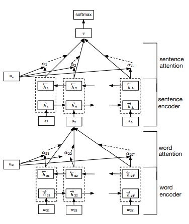
Appl. Sci. 2021, 11, 6113                                                                                           2 of 25

                            of the algorithms for selected datasets. In other studies, evaluation has been performed for
                            texts oriented in a particular domain [6,7].
                                 The contribution of this paper is the proposed HWAN method, which extends the
                            HAN model by including statistical features of the text in the latent representation, thus
                            improving the text classification performance in four out of five datasets. The experiments
                            conducted show that it is possible to improve the quality of document representation by
                            incorporating statistical features learned on a large external corpus.
                                 This paper is structured as follows: In Section 2.1, natural language processing meth-
                            ods are described. In Sections 2 and 3 consecutively, statistical models and deep neural net-
                            works are presented. State-of-the-art models are presented in Section 4. Section 5.1 describes
                            the datasets used for the evaluation of the presented algorithms. The experiment setup is
                            presented in Section 5 and comparison results in Section 6. Section 7 presents our approach
                            for the improvement of a Hierarchical Attention Network that is state-of-the-art for the
                            neural representation of a text. Section 8 discusses the achieved results. We finalise our
                            paper with the conclusions section.

                            2. Statistical Models
                                 We start our survey with a brief description of text preprocessing methods.We then
                            present text representation methods based on statistical algorithms.

                            2.1. Natural Language Preprocessing
                                  A document may be considered a sequence of characters not separated by punctuation
                            marks or spaces, which is an obstacle to the further processing of the document. For this
                            purpose, text segmentation methods are used, which involve partition of the text into words
                            and punctuation marks or dividing documents into utterances. In general, for languages
                            with specified utterance boundaries, segmentation can be performed by splitting texts by
                            punctuation marks or apostrophes, but there are cases where this simple rule does not
                            work, for example, with abbreviations or possessives. This process is essential for most
                            text representation algorithms that operate on single words or tokens.
                                  The noise can be reduced by limiting the size of the dictionary. This can be achieved
                            by different methods (described further), but during preprocessing it can be done by
                            simplifying different inflexion forms of the same word. Three methods are used for this
                            purpose: morphological analysis, lemmatisation and stemming. Morphological analysis
                            is a method of natural language analysis, which provides information on grammatical
                            properties and brings words into basic forms. The second method is based on simplifying
                            words by reducing their inflected forms, for instance, “better” → “good”. This method is
                            usually used when processing languages with rich flexion, for example, Polish. The last
                            method of reducing vocabulary size is stemming, which brings words into their basic form,
                            for example, “running”, “runs”, “ran” → “run”.
                                  Documents are usually gathered from different sources and in different data formats,
                            such as XML and HTML. Thus, during processing, the format of texts should be unified.
                            Usually, they contain special characters, for example, text decorations used on Internet
                            forums or e-mail addresses, which should be removed to reduce the bias of machine
                            learning models.
                                  In natural language, some words are required by language syntax but they do not
                            carry much information. They are often the most frequent words in a given language
                            and are often removed from texts to reduce vocabulary size, accelerate computations and
                            reduce bias. Examples of stop words in English are: “the”, “a”, “an”. The drawback of this
                            step is spoiling the syntax properties of text.

                            2.2. Bag of Words
                                Bag of words (BoW) [8] is the simplest form of statistical representation of text. In this
                            method, a document is represented by a set of words with associated occurrence frequency.
                            An important drawback of this representation is an absence of word order and a lack of
Appl. Sci. 2021, 11, 6113                                                                                          3 of 25

                            context. To reduce the size of the resulting vectors, generally the following preprocessing
                            steps are applied: stop words removal and lemmatization or stemming. To mitigate the
                            lack of context, one can use n-grams instead of word frequencies, for example, bigrams
                            or trigrams.
                                  Because of its simplicity and speed, it is often used as a preprocessing stage in more
                            advanced statistical methods. However, it is limited in processing complex relations
                            between documents and exploiting semantic information.
                                  BoW can be extended by using weighting schemes that relate documents with words.
                            One of the most popular extensions is Term Frequency–Inverse Document Frequency
                            (TFIDF) [9,10], a statistical method for computing the weights of words based on the fre-
                            quency of their occurrence among documents in a dataset. For all words in the corpus, the
                            ratio of inverse frequency to a number of all documents containing this word is calculated.
                            Terms with the highest value of TFIDF weight usually characterize the document well.

                            2.3. Latent Semantic Analysis
                                  Latent Semantic Analysis (LSA) [11] is a statistical method used for high dimensional
                            data. It performs singular value decomposition (Appendix A) of the original matrix, a
                            word–document co-occurrence matrix in the case of documents.his results in a more dense,
                            lower-dimensional representation, and is called latent semantic space.
                                  Let us denote a collection of N documents D = d1 , d2 , . . . , d N with words w from
                            dictionary V of size M, where V = w1 , w2 , . . . , w M . By ignoring the order of words, we
                            can represent those data in a word–document co-occurrence matrix Σ of size N × M with
                            values Z = z(di , w j )i,j . Function z denotes the frequency of word w in document d or its
                            TFIDF weight.
                                  To compute the similarity between two words, the dot product of the i-th column and
                            the j-th row of matrix Σ is calculated because it contains words and their weights in latent
                            semantic space. To calculate the similarity between two documents, the dot product of the
                            i-th column and the j-th row of matrix ΣV is computed.
                                  The original co-occurrence matrix is usually sparse but vectors computed using singu-
                            lar value decomposition are dense. It is possible to create valuable representations of two
                            documents even when they do not have common words, because synonyms and ambigu-
                            ous words are transformed similarly. Due to dimension reduction of the representation
                            vectors, similar words are merged and infrequent words are filtered out. This feature works
                            only in case when the averaged meaning of words is close to the original. In other cases, it
                            may introduce noise to the model.

                            2.4. Latent Dirichlet Allocation
                                  Latent Dirichlet Allocation (LDA) [12] is an algorithm representing documents as a
                            mixture of topics based on the probability of a word belonging to those topics. The method
                            can be described in a few steps. For every document, parameters α and β are computed
                            according to the known a priori number of topics, denoted as T, where α is the probability
                            distribution assignment of documents to topics and β is the probability distribution of
                            assignment of words to topics. Afterwards, for each document d parameter θi that is the
                            probability distribution of topic assignment in document i is drawn from the Dirichlet dis-
                            tribution parametrized by α. Next, for each topic parameter φt , the probability distribution
                            of word assignment to topic t is drawn. Afterwards, for each word j in each document i,
                            topic zi,j is drawn from multinomial distribution parametrized by θi .
                                  In the beginning, it is necessary to prepare data for the LDA algorithm. A dictionary V
                            of size M and a matrix of size D × max( N ) are created, where D is a number of documents
                            and max( N ) is the maximum length of a document in terms of the number of words among
                            all documents. The next step is to randomly assign topics to words and to calculate the
                            frequency of assignments of each word to each topic. Then, a matrix of size M × T of the
                            initial probability distribution of words over topics is computed. By analogy, the matrix of
                            size D × T of the probability of assigning documents to topics is calculated.
Appl. Sci. 2021, 11, 6113 4 of 25
Instead of sampling from multinomial distribution, the Gibbs sampling algorithm [12]
is often used (Appendix B).
After the Gibbs sampling algorithm finishes, the probability distribution of the assign-
ment of the document to one of T topics can be calculated by summing a number of words
assigned to each topic.
3. Deep Neural Networks
In recent years, the usage of neural networks for text representation has shown some
advantages over the statistical approaches. In this section, methods based on deep neural
networks are presented.
3.1. Partition-Smooth Inverse Frequency
Intuition suggests that longer spans of text could be represented based on a repre-
sentation of each word and its context. Using pre-trained models, such as Global Vectors
(GloVe) [13] or word2vec [14], we can use word representations, which retain much of
the syntactic and semantic relations in their projection space. The document consists of
multiple utterances that contain multiple words. This hierarchical structure is reflected in
many algorithms that process long texts, for example, the Hierarchical Attention Network.
Averaging word vectors is a simple method for representing long text, but its draw-
back is a variety of words’ semantic meaning. The resulting representation is the mean of
all components, which for long texts provides similar points in multidimensional space.
Averaging leads to a loss of syntax and semantic information encoded into words’ repre-
sentations. Partition-Smooth Inverse Frequency (P-SIF) is a method of weighted averaging
according to a text topic, which mitigates these drawbacks.
In general, vectors averaging relies on replacing all words with their numerical represen-
tations. Afterwards, the concatenation of the dot product of every word with topic weights
results in a matrix. Next, matrices are averaged, resulting in document representation.
Let us denote a corpus consisting of D documents, a dictionary as V and a weights
matrix as W, which represents the probability of assignment of a word to one of the topics.
Let us denote p(w) as the probability of the occurrence of a word w in the corpus and
K = 3 as the number of topics. For every word w from dictionary V, a vector of parameters
of membership degree αw,1 , . . . , αw,K to each topic K is computed. Let us assume that
document d consists of word vectors v1 , v2 , . . . , vn , where n is the length of the document
in number of words. Document representation, presented in Formula (1), is calculated
as a concatenation of weighted sums of word vectors for every topic where operator ⊕
represents vector concatenation:
n n n n
D = ( ∑ vi × wi1 ) ⊕ ( ∑ vi × wi2 )... ⊕ ...( ∑ vi × wiK ) = ⊕kK=1 ( ∑ vi × wik ) (1)
i =1 i =1 i =1 i =1
The resulting matrix has size K × M, where M is the word vectors dimension. Ac-
cording to simple word vectors averaging, which results in a 1 × M matrix, the P-SIF
algorithm results in a bigger dimension concerning document topics, which is important
for long texts.
In the training procedure [15], first, word vectors from the dictionary are trained,
followed by the creation of word topics vectors and, finally, the re-weighting process.
Formula (2) presents how to compute a word vector for given sparsity parameter k and up-
~ 1, A
per limit m for a list of normal vectors A ~ 2 , ..., A~m , where at least k parameters αw1 , ..., αwm
are non zero and η~w denotes the noise vector.
m
v~w = ∑ αwj A~ j + η~w . (2)
j =1
In the first phase, sparse coding was used [16] but this step can be skipped by assigning
pre-trained word representations, as was done in this study.Appl. Sci. 2021, 11, 6113 5 of 25
To train word vectors for each word w, K different topic vectors cv~wk of size M are
created by computing the dot product of a word vector with parameters αw,k for each topic,
as presented in Formula (3).
cv~wk = v~w × αwk . (3)
Afterwards, the concatenation of all K word topics vectors into matrix tv~w , represent-
ing the topic–word relation of size K × M, is calculated as presented in Formula (4).
tv~wk = ⊕kK=1 cv~wk . (4)
In the last phase, weights for words matrices t~vi are calculated according to Formula (5),
using smooth inverse frequency formula ( a+ pa(w) ), where parameter a controls the shape of
the weighting function.
a
v~dn = ∑ tv~w . (5)
w∈d
a + p(w)
n
Finally, common context from averaged document vectors is removed by deleting the
first principal component, calculated by using PCA [17]. This operations is defined by the
Formula (6), where ~u is the first singular vector:
v~dn = v~dn − ~u~u T v~dn . (6)
3.2. Doc2Vec—Distributed Memory Model of Paragraph Vectors
Paragraph Vector is a method for the representation of longer, variable-length texts
such as phrases, sentences or whole documents [18]. In this model, the task used for
training is to predict the words in a paragraph. A concatenation of a paragraph vector,
along with several vectors of words found in the context, is performed and then the most
likely word matching the context is inferred, as presented in Figure 1. Paragraph vectors
are unique, while word vectors are shared between paragraphs. The model template is
a modified version of the Continuous Bag of Words model [19,20], which is computed
according to Formula (7), where U and b are the parameters of the so f tmax function, h is
the concatenation or averaging function of the word vectors obtained from the matrix W of
words in the vocabulary, and the parameter k is the size of the context window.
y = Uh(wt−k , ..., wt+k ; W ) + b. (7)
Each paragraph is represented by a corresponding column in the matrix D, and each
word vector is represented by a corresponding column in the matrix W. The paragraph
vector and the context word vectors are then averaged or concatenated, and the next context
word is predicted. An additional element that appears in the model is the paragraph token,
which can be understood as the next word. It acts as a memory that stores missing words
from the context of the paragraph topic. This is where the name Distributed Memory Model
of Paragraph Vectors comes from. The size of the context is an application-specific parame-
ter. The paragraph vector is shared among all contexts generated by the sliding context
window on the paragraph. The word vector matrix W is shared between paragraphs.
Figure 1. Distributed Memory Model of Paragraph Vectors [18].Appl. Sci. 2021, 11, 6113 6 of 25
The architecture of the model is based on a single-layer neural network. The input
parameters are words from the context window in the form of a one-hot vector or as a
dictionary mapped index and a paragraph index. The output parameter is the predicted
word belonging to the context, analogous to Continuous Bag of Words.
The algorithm has two phases of operation: Phase one, which consists of training the
word vectors W, and training the network weights and the paragraph vectors D, and Phase
two, in which the model learns new paragraphs by adding their vectors to the matrix D
and training the network without updating the matrix W or the network weights. Inference
uses the resulting matrix of paragraph vectors D. An important feature of the model is
the use of unlabelled training datasets. They inherit the vector semantics of the obtained
representations from the Continuous Bag of Words model and also take into account the
order and contextuality of the words.
3.3. Doc2Vec—Distributed Bag of Words Paragraph Vector
The Paragraph Vector Distributed Bag of Words method, analogous to Skip-gram, pre-
dicts the context based on some token. In the case of Skip-gram, this is the word central to the
context and, in the case of the Distributed Bag of Words Paragraph Vector, it is the paragraph
vector. In practice, we sample the context window then randomly select a word from the
context and perform classification with the given paragraph, as presented in Figure 2.
Figure 2. Distributed Bag of Words Paragraph Vector [18].
The architecture of the model is based on a single-layer neural network. The input
parameter is the paragraph vector and the output parameters are words belonging to the
context, analogous to Skip-gram.
Unlike the Distributed Memory Model of Paragraph model, it is much simpler and
requires fewer data to be stored but its performance is slightly worse [18].
3.4. Hierarchical Attention Network
Hierarchical Attention Network (HAN) [21] is a deep neural network model used
to represent documents employing the hierarchical structure of documents. Due to the
varying amount of information that words or phrases carry depending on the context, two
levels of attention mechanism were used—first at the word level and second at the sentence
level (Figure 3). The attention mechanism additionally carries the ability to monitor which
word or phrase contributed the most to a particular decision made by the model, which
helps us to understand decisions made by the model. The implementation used in our
experiments was based on the publicly available implementation repository [22].Appl. Sci. 2021, 11, 6113 7 of 25
Figure 3. Hierarchical Attention Network [21].
The HAN model consists of a word encoder, a word attention layer, a sentence encoder
and a sentence attention layer. Suppose a document contains L sentences denoted by si ,
and each sentence contains Ti words. The wit of the range t in [1, T ] represents the words
in the ith sentence. Given a sequence of word vectors wit , t in [1, T ], we perform their
encoding by the matrix We , xij = We wij . Using bidirectional GRU networks [23], we
obtain the encoded vectors by summing the output information from both directions, thus
including the context information. Latent states of the model are calculated according to
Formula (8). The bidirectional GRU layer contains a forward part ~f , which, based on the
←
−
sentence si , processes words from wi1 to wiT and a backward part f , which processes
words from wiT to wi1 .
xit = We wit , t ∈ [1, T ]
−−−−→
h~it = GRUxit , t ∈ [1, T ] (8)
←− ←−−−−
hit = GRUxit , t ∈ [ T, 1].
The encoded expressions are obtained as a concatenation of the hidden states of the
network in both directions according to Formula (9).
←−
hit = [h~it , hit ]. (9)
Because words affect the meaning of a sentence to varying degrees, an attention
mechanism was introduced to extract keywords and aggregate them to form a sentence
vector. Formula (10) presents HAN attention, where u is the attention state for each word,
α is its weight, and s is the initial state of the encoded sentence obtained by summing the
weighted states of the individual words.
uit = tanh(Ww hit + bw )
αit = so f tmax (uitT uw ) (10)
si = ∑tT=1 αit hit .
Initially, we feed the word representation hit , obtained in the previous layer, into a
1-layer neural network to obtain its hidden state uit . We then measure the relevance of theAppl. Sci. 2021, 11, 6113 8 of 25
words as the similarity of uit to the context of the words uw and obtain the weights αit with
the function so f tmax. We obtain the sentence representation si as a weighted sum of the
word representations hit .
We obtain the encoded document vector in a similar way, using bidirectional GRU
networks as presented in Formula (11).
~hi = −−−→
GRUsi , i ∈ [1, L]
←− ←−−− (11)
hi = GRUsi , i ∈ [ L, 1].
We obtain an analogously encoded document as a concatenation of hidden network
states in both directions according to Formula (12)
←
−
hi = [~hi , hi ]. (12)
Once again, we apply the attention mechanism, this time to encoded sentences
(Formula (13)), where us is the document context and v is the resulting document vector.
The only difference is the replacement of word representations with sentence representations.
ui = tanh(Ws hi + bs )
αi = so f tmax (uiT us ) (13)
v= ∑tT=1 αi hi .
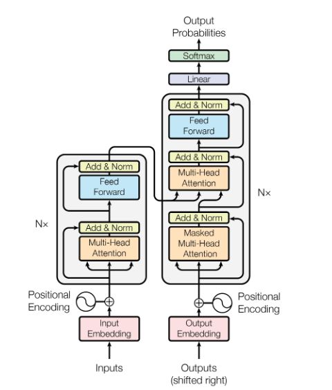
3.5. Bidirectional Encoder Representations from Transformers
Transformer models are designed to pre-train a model on a large set of texts and
then, using transfer learning, attach one output layer and tune it to solve a specific task.
This way, we can easily obtain models that solve a wide range of problems without major
architecture modifications and save resources. The unified architecture of the pre-trained
model applied to different tasks is a distinguishing feature of the Bidirectional Encoder
Representations from Transformers (BERT) model from other models whose architecture is
tailored to the task being solved.
The BERT architecture consists of multiple Transformer layers created based on the
original implementation presented by Ashish Vaswani [24].
The Transformer layer (Figure 4) is based on the encoder–decoder architecture but, un-
like common recurrent networks, it uses feed-forward neural networks along with an
attention mechanism. In the paragraphs below BERT, the base architecture is described.
The encoder consists of a stack of six identical layers. Each layer contains two sub-
layers: a multi-head self-attention mechanism and an element-wise fully-connected feed-
forward network. Each sublayer uses residual connections followed by layer normalization.
Each sublayer has a projection to a 512-dimensional representation.
The decoder also consists of a stack of six identical layers. In addition to the two sub-
layers present in the encoder, a sublayer has been added that performs masked multi-head
attention on the representations obtained from the encoder stack. In this sublayer, similarly
to the encoder, residual connections have been applied along with layer normalization.
The attention model can be described as a vector of n values that represent the mutual
relevance of the words to each other. The multi-head attention (Figure 5) used in this
model consists of eight parallel units. The first layer is a projection layer of Q, K, and V
to a 64-dimensional representation followed by a Scaled Dot-Product Attention function.
The resulting vectors are then multiplied and a linear projection of their product is added
to the final output value.Appl. Sci. 2021, 11, 6113 9 of 25
Figure 4. Transformer block architecture [24]. The left part is the encoder and the right part is
the decoder.
Figure 5. Multi-head Attention [24].
The linear projection of input word vectors is the product of the input vector with vectors of
three weights resulting in vectors Query, Key and Value, denoted by Q, K and V, respectively.
The Scaled Dot-Product Attention function is computed for each input word vector
(Figure 6). The attention value is calculated as follows: for each word, the matrix product
between the vector Qi and the matrix of vectors K of each input word, including the
Attention value for the currently processed word, is computed. The resulting value is then
scaled by dividing by the squared root of the dimension of vector K. The value of the
so f tmax function from the obtained vector of values for the attention value for the i-th
word is then computed, and the product of the obtained values with the V vectors of all
words is then computed. Finally, the sum of the obtained vectors represents the attention
for the i-th word. In this way, attention is computed for all words. The dimension of the
weights used to obtain the Q and K vectors must be equal, while the dimension of the V
vector weights can be arbitrary. Scaled Dot-Product Attention is a function described byAppl. Sci. 2021, 11, 6113 10 of 25
the Formula (14), where QK T is the scalar product of vectors and dK is the dimension of
vector K (Figure 6).
QK T
Attention( Q, K, V ) = so f tmax ( √ )V. (14)
dK
We denote the number of Transformer layers as L, the size of the hidden layer as H,
the size of self-attention heads as A, and the final architecture is taken as L = 24, H = 1024,
A = 16.
Figure 6. Scaled-Dot Product Attention [24].
3.6. Longformer
Longformer [25] is a deep neural network built from Transformer blocks [26] and opti-
mized for the memory requirements. While the most common transformer model—BERT—has
a quadruple relation input sequence length for memory requirements, Longformer has a linear
relation between those parameters. This feature enables the usage of Transformer based models
to handle long spans of text.
In order to optimize the memory consumption of the model, the attention function
was modified, forming an attention pattern (Figure 7). Instead of fully computing the
attention of each pair of tokens, a sliding window method was used, in which attention
is computed for each pair of tokens that are in a window context where its length is less
than the length of the entire input string. Additionally, a global attention mechanism was
introduced. According to this mechanism, attention values for tokens with global attention
are computed between those particular tokens and all tokens from the sliding window
context. As a third possibility, random attention was introduced, in which tokens for which
local attention is computed are randomized.
Figure 7. Different attention schemes [25]. Longformer attention scheme is presented by (d).
It is important to set up global attention correctly when using the model. The authors
of the transformer’s library [27] recommend using the global attention for the token
in text classification problems; for answering questions, the attention should be set to theAppl. Sci. 2021, 11, 6113 11 of 25
question tokens, and in language modelling, the attention should be set to the beginning of
the utterance.
Using the optimized attention block, it is possible to process many times longer texts than
using BERT. BERT-like models can process texts of 512 tokens in length, while Longformer
can handle any length. In the case of the benchmark, a model processing 4096 tokens was
used, but a model that handles up to 16,384 tokens has been also published [28].
4. State-of-the-Art Baseline
The current state-of-the-art models were obtained from the paperswithcode web-
site [29], based on the best performance on the text classification subtask on diverse datasets.
Extensive use of recurrent networks to process sequential data was common before the
Transformer era. An example of such a model is the bidirectional LSTM [30] network [31],
which processes pre-trained word representations. A hierarchical variant of this model is
the HDLTex network [32].
Most models use the Transformer architecture, which has been modified specifically
for the task of document classification on shorter texts. Due to their growing popularity, the
extension of these models, along with additional tricks, were used to process long texts more
efficiently. A simple approach was to fine-tune the BERT model for document classification
by including additional fully connected layers and a so f tmax cost function [33]. A similar
approach was used in the paper “How to Fine-Tune BERT for Text Classification?” [34],
where pre-training was additionally used on a training dataset, followed by fine tuning.
Another architecture based on this architecture is the XLNet [35] autoregressive model,
which uses two-stream self-attention for target-aware representation and, inspired by the
TransformerXL [36], uses relative position encoding.
A different, yet very promising, graph approach is used in many current SOTA
models, such as Massage Passing Attention Networks [37], which is the best model on
the Reuters dataset. In this model, documents are represented as graphs built from a
word co-occurrence matrix and a special node representing the document. In this model,
a sentence representation is obtained by iteratively passing messages between nodes,
and classification is performed on the glued representations of all sentences. A similar
approach was presented in graph-based attention networks [38], which treat documents
as nodes whose representations are vectors obtained by the bag-of-words method on
which a self-attention operation is performed, together with neighbouring nodes. Similar
assumptions were used in the Learnable Graph Convolution Network [39] model, in which
an additional pre-learning step is the selection of a subgraph that allows the graph to be
transformed into grid-like one dimensional data before training and the use of standard
convolution layers. The best models were selected for comparison in the following section
of the paper.
5. Experiment Design
To compare selected methods, one pipeline of training and evaluation for all models
was designed. The first dataset is loaded into program memory. The second step is the
preprocessing of texts. Then, a dataset is split into five parts following a K-fold cross-
validation scheme. The model is trained on a training set of cleaned documents. The final
evaluation is performed after the selected model generates a vector representation of the
documents, which are passed into the classifier. The used classifier is a multi-class SVM
algorithm [40], taking into account the prevalence of unbalanced training sets. After the
procedure is finished, results are averaged and saved. As an evaluation metric, average
overall accuracy was used, which is the percent of correct predictions provided by the
model with standard deviation across all runs. The code for the experiment is publicly
available [41].
The importance of text preprocessing was addressed in the paper [42], where the
authors presented how much preprocessing affects the model output. In conclusion, they
presented general findings: usually, tokenization achieves the same or better results thanAppl. Sci. 2021, 11, 6113 12 of 25
more complex processing, such as coreference. The exception here was the Ohsumed
collection, where there are many medical words, where the most efficient technique was to
treat expressions or groups of words as a single token.
In our evaluation of all datasets following preprocessing, steps were applied: low-
ercasing (except Longformer, which was pre-trained on uncased texts), filtering email
addresses and decorations.
The increase in the maximum length of the processed sequence is due to the increased
VRAM requirements of the GPU cards on which the calculations were performed. The oc-
currence of outliers from the dataset that were many times longer than the mean would
have unnecessarily increased the network size and increased the training time. Due to
the limited hardware resources, it was necessary to limit the size of the neural networks
in order to be able to perform the training. For models with a defined fixed length of
the processed sequence of words and sentences resulting from the architecture of neural
networks and their implementation details, it was decided to conduct the experiment in
two variants. The first is to limit the length of the text to 30 sentences, each with a maximum
of 100 words. The second is to limit the length based on the frequency distribution of
sentences and words in the training datasets and, on this basis, to select the 99th percentile
of the distribution.
The results of the training process for selected training datasets are presented below.
The average accuracy and average training time of the models were measured.
The parameters with which the models were trained are as follows: For BoW and
TFIDF, the dictionary size was not limited; min_df = 1 and max_df = 0.95 were selected
as the number of minimum occurrences of a word and the maximum frequency ratio of
a word in the set. Identical min_df and max_df parameters were also used in the LSA
and LDA models. LSA was run with parameters svd_features = 100, which specify
the number of dimensions after SVD reduction, the number of iterations n_iter = 10.
Similarly, LDA, in which n_components = 100 specifies the number of implicit topics
to which words were assigned, and the number of iterations epochs = 10. The P-SIF
model is parameterised by the number of clusters num_clusters = 40 and the size of the
resulting representation embedding_size = 100. Doc2Vec, DM and DBoW models were
parameterized identically: the number of negative examples negative = 10, projection
size vector_size = 100, context window window = 5 and minimum word frequency
min_count = 1. For the HAN model, the maximum number of sentences and words in
sentences is configuration dependent. In addition to these parameters, the validation
data ratio validation_split = 0.1, batch size equal to 16, and the number of epochs
equal to 100 were used and an unlimited dictionary for statistical features was applied
by parameter max_features = None. For the Longformer model, the number of iterations
was set to epochs = 10 and the batch size was equal to 4. The latter model was trained
using full precision fp16 = False because of instability issues. As a pre-trained word
vector, GloVe [14], with 100 dimension size, was selected.
Limiting the length of the processed text to the 99th percentile for each set was done by
analyzing the frequency distribution of sentences and words in the sentences, from which
the corresponding values were determined and used in the training process. Data regarding
the state-of-the-art models were retrieved from the website [29].
5.1. Datasets
To evaluate selected text representation algorithms, five different datasets were se-
lected [43,44] The selection of the datasets was based on a difference of the parameters:
dataset size, document length, domain, the variance of document length and the variance
in a number of samples in each class. The datasets used in the experiments are described
briefly below.Appl. Sci. 2021, 11, 6113 13 of 25
5.1.1. BBCSport
BBCSport [43] consists of 737 documents about sports events published on the BBC
website during the years 2004–2005. Texts are grouped into five classes: athletics, rugby,
cricket, football and tennis. Data are not divided into train and test sets; therefore, a method
of evaluation is cross-validation. Class frequency distribution is presented on Figure 8,
whereas the distribution of word frequency is presented in Figure 9.
Figure 8. Class frequency distribution for BBCSport.
Figure 9. Distribution of words frequency in BBCSport.
The dataset is imbalanced in terms of the number of samples for each class and it has
a shape of normal distribution. The most frequent class is class two, the rarest are classes
zero and four.
5.1.2. BBC
BBC consists of 2225 documents published on the BBC website in the years 2004–2005.
Texts are grouped into five categories: business, entertainment, politics, sport and tech.Appl. Sci. 2021, 11, 6113 14 of 25
Data are not divided into train and test sets, therefore a method for evaluation is cross-
validation.
The dataset is balanced in terms of the number of samples for each class , as presented in
Figure 10. According to Figure 11, the documents are in the range from 100 to 5000 words length.
Figure 10. Class frequency distribution for BBC.
Figure 11. Distribution of words frequency in BBC.
5.1.3. Reuters
Reuters consists of 15,437 documents published on the Reuters website. Texts are
grouped into 91 categories and the dataset is divided into train and test sets. Class frequency
distribution is presented in Figure 8, whereas the distribution of the word frequency is
presented in Figure 9.
The dataset is imbalanced in terms of the number of samples for each class. According
to Figure 12, three classes dominate the dataset in terms of frequency. Documents are
usually between 100 and 5000 words in length, as presented in Figure 13.Appl. Sci. 2021, 11, 6113 15 of 25
Figure 12. Class frequency distribution for Reuters.
Figure 13. Distribution of words frequency in Reuters.
5.1.4. 20Newsgroups
20Newsgroups [45] consists of 20,417 documents from the Usenet website newsgroups
collection. Texts are grouped into 20 categories and the dataset is not divided into train
and test sets; therefore, the method of evaluation is cross-validation.Appl. Sci. 2021, 11, 6113 16 of 25
Documents are usually between a few and 10,000 words in length. Some samples are
much longer than the average number of words, according to Figure 14. The dataset is
balanced in terms of the number of samples for each class, as presented in Figure 15.
Figure 14. Class frequency distribution for 20Newsgroups.
Figure 15. Distribution of words frequency in 20Newsgroups.
5.1.5. Ohsumed
Ohsumed [46] consists of medical abstracts from the MeSH category from the year
1991 and contains 20,000 documents divided into train and test sets. Texts are grouped into
23 categories of cardiovascular diseases.
The dataset is imbalanced in terms of sample number in each class. According to the
chart in Figure 16, three classes dominate the dataset in terms of frequency, as presented inAppl. Sci. 2021, 11, 6113 17 of 25
Figure 16. The length of documents is usually between 200 and 3000 words, according to
Figure 17.
Figure 16. Class frequency distribution for Ohsumed.
Figure 17. Distribution of word frequency in Ohsumed.
6. Results of Representations Comparison
In this section, detailed results of representations comparison in terms of averaged
overall classification accuracy are shown in Table 1. Table 2 presents the training times
required for training each model.
It can be seen from Table 1 that the statistical methods achieve results that are compara-
ble to the selected neural methods. For the Reuters and Ohsumed collections, the statistical
baseline achieved the best results, which are, however, significantly worse than the state-
of-the-art. This may be related to the characteristics of the collections, such as the high un-
balance of class examples. For five datasets—20Newsgroups, BBC and BBCSport—neural
networks utilizing the attention mechanism outperformed the statistical baseline methods.
For the BBCSport dataset model, HAN achieved 100% accuracy, outperforming the current
state-of-the-art (based on the paperswithcode website).Appl. Sci. 2021, 11, 6113 18 of 25
Among the methods that performed better than the statistical baseline are the networks
based on the attention mechanism—HAN and Longformer. Among these two methods,
the HAN method achieved better accuracy and the model inference time is significantly
shorter compared to the model based on the Transformer architecture (Table 2), and
therefore this model was chosen for further analysis and modification.
Table 1. Averaged overall classification accuracy (in percent); cross-validation for Ohsumed, BBC and BBCSport, test–train
split for Reuters and 20Newsgroups. The maximum length of input data for HAN was set at 30 utterances 300 words each.
Numbers in bold denotes results better than BoW and TFIDF or the best overall result.
Model Reuters Ohsumed 20Newsgroups BBC BBCSport
BoW 83.42 , σ = 0.0 60.25, σ = 0.0 71.72, σ = 0.0042 97.03, σ = 0.0077 96.88, σ = 0.0127
TFIDF 75.58, σ = 0.0 56.44, σ = 0.0 85.55, σ = 0.0008 97.84, σ = 0.0037 98.51, σ = 0.0117
LSA 64.12, σ = 0.0017 35.72, σ = 0.0012 71.76, σ = 0.0053 96.90, σ = 0.0030 97.83, σ = 0.0117
LDA 52.91, σ = 0.0093 20.07, σ = 0.0036 60.90, σ = 0.0102 93.08, σ = 0.0056 92.80, σ = 0.0419
P-SIF 62.61, σ = 0.0016 34.33, σ = 0.0015 63.41, σ = 0.0057 95.33, σ = 0.0063 94.70, σ = 0.0267
Doc2Vec-DM 79.81, σ = 0.0013 58.66, σ = 0.0021 75.25, σ = 0.0075 96.63, σ = 0.0071 97.29, σ = 0.0096
Doc2Vec-DBoW 82.65, σ = 0.0006 59.48, σ = 0.0006 82.52, σ = 0.0040 97.35, σ = 0.0046 97.96, σ = 0.0096
HAN 81.33, σ = 0.0046 54.39, σ = 0.0029 89.57, σ = 0.0066 99.24, σ = 0.0046 100, σ = 0.0
Longformer base 79.90, σ = 0.0042 53.88, σ = 0.0077 81.33, σ = 0.0054 98.20, σ = 0.0028 99.32, σ = 0.0061
SOTA 97.44 [37] 75.86 [47] 88.6 [48] 99.59 [37]
Table 2. Average total training and inference time in seconds.
Model Reuters Ohsumed 20Newsgroups BBC BBCSport
BoW 27.16 20.42 68.50 5.79 1.20
TFIDF 0.95 0.95 2.31 0.54 0.11
LSA 25.51 45.82 38.70 8.48 1.88
LDA 363.29 179.01 947.30 193.08 69.32
P-SIF 363.14 356.04 777.95 164.63 71.26
Doc2Vec-DM 225.34 247.14 311.22 42.67 13.67
Doc2Vec-DBoW 183.42 190.18 241.81 34.31 11.94
HAN 3611.17 2816.97 5931.19 771.30 254.61
Longformer base 64,935.80 74,314.70 105,622.34 14,396.79 4919.38
7. Our Approach—Hierarchical Weighted Attention Network
By analysing the fine-tuned models using the Local Interpretable Model-agnostic
Explanations (LIME) algorithm [49], insights were gained into how the best methods work.
Using the LIME algorithm, it was observed that a hierarchical attention network
performs well with texts whose topic is not sewn into the statistical features of the text
itself but is derived from the meaning of the text. However, there are cases where the
HAN model assigns too much attention to certain words, as a result of which it incorrectly
guesses the topic, while the statistical TFIDF approach performs correctly.
To overcome the weaknesses of the hierarchical attention network and to enrich
them with statistical features, we propose the Hierarchical Weighted Attention Network
(HWAN). The architecture of this neural network model is based on a hierarchical attention
network enriched with the statistical values of a text’s features.
Additionally, for each input token, the value of the statistical feature of a given word is
passed as an input parameter of the model. For each word, its attention value is calculated,
then, together with the statistical features (BoW, TF or TFIDF value for given words),
a selected operation is performed on them (as shown in Figure 18 in the section “Word
attention”). In the image, the statistical features are successively called w21 , w22 , up to w2T ,
and the operation is denoted by the tensor product symbol. The result of this operation is
a latent variable of a single sentence and it is passed to the document level bidirectional
Long-Short Term Memory [30] layer. After that, there is the so f tmax layer, which calculatesAppl. Sci. 2021, 11, 6113 19 of 25
the attention score for the whole document. Our study examined three different operations:
concatenation (denoted in Tables 3 and 4 as concat), addition (add) and multiplication (mul)
of word attention and statistical features. The models are named as follows: the first part
of the name specifies the type of statistical feature and the second part specifies the type
of information appending operation. Assuming that the statistical feature is BoW and the
operation is add, we get the name BoW + add. The model parameters are the same as for
the baseline HAN model.
Figure 18. The architecture of our Hierarchical Weighted Attention Network.
Table 3. Averaged overall classification accuracy (in percent) for HAN and variants of HWAN; cross-validation for Ohsumed,
BBC and BBCSport, test-train split for Reuters and 20Newsgroups. Restricting input length at 30 sentences 100 words each.
Numbers in bold denotes results better than baseline HAN model.
Model Reuters Ohsumed 20Newsgroups BBC BBCSport
HAN 81.33, σ = 0.0046 54.39, σ = 0.0029 89.57, σ = 0.0066 99.24, σ = 0.0046 100, σ = 0.0
TFIDF + add 82.85, σ = 0.0022 55.64, σ = 0.0027 88.68, σ = 0.0030 99.69, σ = 0.0011 100, σ = 0.0
TFIDF + mul 72.76, σ = 0.0051 34.03, σ = 0.0313 70.51, σ = 0.0168 98.88, σ = 0.0045 69.51, σ = 0.1957
TFIDF + concat 82.44, σ = 0.0011 53.33, σ = 0.0044 85.40, σ = 0.0086 99.64, σ = 0.0027 99.59, σ = 0.0054
TF + add 82.81, σ = 0.0014 55.39, σ = 0.0032 88.68, σ = 0.0038 99.60, σ = 0.0026 99.73, σ = 0.0054
TF + mul 73.50, σ = 0.0057 37.61, σ = 0.0145 72.41, σ = 0.0088 99.01, σ = 0.0066 87.29, σ = 0.1613
TF + concat 82.44, σ = 0.0017 53.00, σ = 0.0042 85.86, σ = 0.0051 99.55, σ = 0.0038 100, σ = 0.0
BOW + add 82.88, σ = 0.0012 55.10, σ = 0.0038 88.01, σ = 0.0131 98.92, σ = 0.0048 98.51, σ = 0.0079
BOW + mul 81.97, σ = 0.0011 52.20, σ = 0.0234 71.51, σ = 0.0079 99.51, σ = 0.0030 100, σ = 0.0
BOW + concat 82.46, σ = 0.0017 51.18, σ = 0.0081 75.08, σ = 0.0101 99.19, σ = 0.0048 99.32, σ = 0.0043Appl. Sci. 2021, 11, 6113 20 of 25
Table 4. Averaged overall classification accuracy (in percent) for HAN and variants of HWAN; cross-validation for Ohsumed,
BBC and BBCSport, test-train split for Reuters and 20Newsgroups. Restricting input length at 99-th percentiles of the
number of sentences and words. Numbers in bold denotes results better than baseline HAN model.
Model Reuters Ohsumed 20Newsgroups BBC BBCSport
HAN 81.79, σ = 0.0015 51.19, σ = 0.0061 87.17, σ = 0.0060 99.55, σ = 0.0014 100.0, σ = 0.0
TFIDF + add 82.13, σ = 0.0016 51.00, σ = 0.0069 87.43, σ = 0.0061 99.01, σ = 0.0046 99.46, σ = 0.0051
TFIDF + mul 58.51, σ = 0.0812 25.15, σ = 0.0404 43.54, σ = 0.3148 79.60, σ = 0.2893 62.70, σ = 0.3
TFIDF + concat 82.06, σ = 0.0021 51.66, σ = 0.0054 88.14, σ = 0.0045 98.79, σ = 0.0046 99.46, σ = 0.0051
TF + add 82.03, σ = 0.0028 51.20, σ = 0.0112 87.47, σ = 0.0041 99.46, σ = 0.0044 98.11, σ = 0.0224
TF + mul 61.94, σ = 0.0138 23.29, σ = 0.0967 69.57, σ = 0.0439 97.80, σ = 0.0166 96.07, σ = 0.0349
TF + concat 80.26, σ = 0.0029 46.57, σ = 0.0108 78.49, σ = 0.0078 99.01, σ = 0.0068 99.46, σ = 0.0051
BoW + add 81.90, σ = 0.0041 40.17, σ = 0.0056 77.62, σ = 0.0176 99.24, σ = 0.0061 96.88, σ = 0.0220
BoW + mul 82.59, σ = 0.0016 50.39, σ = 0.0270 82.22, σ = 0.0168 98.97, σ = 0.0030 32.09, σ = 0.2865
BoW + concat 81.57, σ = 0.0013 39.27, σ = 0.0147 79.55, σ = 0.0117 98.79, σ = 0.0056 99.05, σ = 0.0069
Comparison of HAN an HWAN
To evaluate our approach, we performed experiments aiming to compare the HAN
method with different variants of the HWAN method. It was observed that limiting the
length of text processed by the model degraded the performance of the HWAN model to a
lesser extent. We also noted that the Reuters dataset, for almost all configurations of the
HWAN model, performed better for both restricted and not-restricted document length.
The worst results came from the operation of multiplying statistical features and neural
network excitation, as can be seen in Tables 3 and 4.
For the limited length of the text processed, the best results were obtained by adding
statistical features whose results did not vary much. For the unlimited length of processed
text, the best results were achieved for concatenation and addition TFIDF features, with a
maximum difference of 0.71 percentage points in their results, and for the addition of
TF features.
As shown in Tables 3 and 4, the multiplication operation degraded the resulting
representations, which affected the quality of further processing, resulting in a drastic
decrease in the performance of these representations in the classification task, especially
for the BBCSport dataset.
For further comparison, the TFIDF + add variant was denoted as HWAN, as it produced
the best performance for the majority of datasets.
For the Reuters dataset, the best performance was achieved by the baseline model
BoW (83.42%). The other models performed worse: TFIDF (−7.84 percentage point.),
LSA (−19.30 percentage point.), LDA (−30.51 percentage point.), P-SIF (−20.81 percent-
age point.), Doc2Vec-DM (−3.61 percentage point.), Doc2Vec-DBoW (−0.77 percentage
point.), HAN (−2.09 percentage point.), HWAN (−0.57 percentage point.), Longformer
(−3.52 percentage point.).
For the Ohsumed dataset, the best performance was achieved by the BoW (60.25%)
model. The other models performed worse: TFIDF (−3.81 percentage point.), LSA
(−24.53 percentage point.), LDA (−40.18 percentage point.), P-SIF (−25.92 percentage
point.), Doc2Vec-DM (−1.59 percentage point.), Doc2Vec-DBoW (−0.77 percentage point.),
HAN (−5.86 percentage point.), HWAN (−4.61 percentage point.), Longformer (−6.37 per-
centage point.).
For the 20Newsgroups dataset, the best performance was achieved by the HAN
(89.57%) model. TFIDF (−4.02 percentage point.) performed slightly worse. The other
models performed worse: BoW (−17.85 percentage point.), LSA (−17.81 percentage point.),
LDA (−28.67 percentage point.), P-SIF (−26.16 percentage point.), Doc2Vec-DM (−14.32
percentage point.), Doc2Vec-DBoW (−7.05 percentage point.), HWAN (−0.89 percentage
point.), Longformer (−8.24 percentage point.).Appl. Sci. 2021, 11, 6113 21 of 25
For the BBCSport dataset, the best performance was achieved by the HAN and
HWAN models (100.00%). A result better than baseline was also achieved by Longformer
(−0.68 percentage point.).
For the BBC dataset, the best performance was achieved by the HWAN model (99.69%).
A result better than baseline was also achieved by HAN (−0.45 percentage point.) and
Longformer (−0.68 percentage point.).
8. Discussion
In summary, for three of the five datasets, the HAN and HWAN models performed
the best, for the other two the BoW method produced better results. The HAN and
HWAN models dominate the other methods in terms of performance due to their attention
mechanism. The models use this mechanism to select the most semantically relevant parts
of the text and determine the document class based on them, which is similar to what
humans do when reading the text. Longformer’s results are worse than expected. Intuition
suggests that the attention mechanism should improve the quality of text representations
and ease classification. Probably due to the longer input sequence, Longformer performs
worse than HAN, as shown in Table 1. On the other hand, for the Reuters and Ohsumed
collections, simple statistical methods, such as a BoW or TFIDF, perform better. For data
with domain-specific vocabulary, the BoW method performs the best, probably due to
the absence of some words in the vocabulary of methods based on pre-trained word
representations. The LDA model performs significantly worse on bigger datasets with
a larger number of classes. Methods grouped under the name doc2vec achieved the
best results for the Ohsumed dataset, excluding the baseline. The doc2vec-DBoW model,
in particular, performs very well for all datasets, slightly worse than baseline.
Based on the difference in the results for the HAN and HWAN models in Tables 1 and 5,
it can be observed that the deterioration of the results for the Ohsumed and BBC datasets is
a result of the fact that the relevant information for the classification problem is included in
the initial parts of the documents. Increasing the maximum input processed string results
in a decrease of accuracy, which involves processing a longer text, making it more difficult
for the model to extract significant information.
Table 5. Averaged overall classification accuracy (in percent); cross-validation for Ohsumed, BBC and BBCSport, test-train
split for Reuters and 20Newsgroups. The maximum length of input data for HAN and HWAN was set at 30 utterances
300 words each. Numbers in bold denotes results better than BoW and TFIDF or the best result.
Model Reuters Ohsumed 20Newsgroups BBC BBCSport
BoW 83.42, σ = 0.0 60.25, σ = 0.0 71.72, σ = 0.0042 97.03, σ = 0.0077 96.88, σ = 0.0127
TFIDF 75.58, σ = 0.0 56.44, σ = 0.0 85.55, σ = 0.0008 97.84, σ = 0.0037 98.51, σ = 0.0117
LSA 64.12, σ = 0.0017 35.72, σ = 0.0012 71.76, σ = 0.0053 96.90, σ = 0.0030 97.83, σ = 0.0117
LDA 52.91, σ = 0.0093 20.07, σ = 0.0036 60.90, σ = 0.0102 93.08, σ = 0.0056 92.80, σ = 0.0419
P-SIF 62.61, σ = 0.0016 34.33, σ = 0.0015 63.41, σ = 0.0057 95.33, σ = 0.0063 94.70, σ = 0.0267
Doc2Vec-DM 79.81, σ = 0.0013 58.66, σ = 0.0021 75.25, σ = 0.0075 96.63, σ = 0.0071 97.29, σ = 0.0096
Doc2Vec-DBoW 82.65, σ = 0.0006 59.48, σ = 0.0006 82.52, σ = 0.0040 97.35, σ = 0.0046 97.96, σ = 0.0096
HAN 81.33, σ = 0.004 54.39, σ = 0.0029 89.57, σ = 0.0066 99.24, σ = 0.0046 100, σ = 0.0
HWAN 82.85, σ = 0.0022 55.64, σ = 0.0027 88.68, σ = 0.0030 99.69, σ = 0.0011 100, σ = 0.0
Longformer base 79.90, σ = 0.0042 53.88, σ = 0.0077 81.33, σ = 0.0054 98.20, σ = 0.0028 99.32, σ = 0.0061
SOTA 97.44 [37] 75.86 [47] 88.6 [48] 99.59 [37]
For the limited length of the processed text string, the HWAN model performed better
than HAN for the Reuters, Ohsumed and BBC datasets, as shown in Table 1, due to the
inclusion of TFIDF weights in the word representation, which allowed the relevance of indi-
vidual words to be highlighted to a greater extent. Potentially, the use of statistical features
computed from a large external corpus can improve HWAN performance, as shown by the
difference in results in Tables 3 and 4 for unlimited and limited processed text lengths for
the HAN and HWAN models, where the statistical model had access to full documents.You can also read