Statistical Analysis on Brain Surfaces
←
→
Page content transcription
If your browser does not render page correctly, please read the page content below
Statistical Analysis on Brain Surfaces

                                                           Moo K. Chung, Jamie L. Hanson, Seth D. Pollak

                                                                  University of Wisconsin-Madison, USA

                                                                             mkchung@wisc.edu

                                                  Abstract. In this paper, we review widely used statistical analysis frame-
arXiv:2203.06665v1 [q-bio.NC] 13 Mar 2022

                                                  works for data defined along cortical and subcortical surfaces that have
                                                  been developed in last two decades. The cerebral cortex has the topol-
                                                  ogy of a 2D highly convoluted sheet. For data obtained along curved
                                                  non-Euclidean surfaces, traditional statistical analysis and smoothing
                                                  techniques based on the Euclidean metric structure are inefficient. To
                                                  increase the signal-to-noise ratio (SNR) and to boost the sensitivity of
                                                  the analysis, it is necessary to smooth out noisy surface data. However,
                                                  this requires smoothing data on curved cortical manifolds and assign-
                                                  ing smoothing weights based on the geodesic distance along the surface.
                                                  Thus, many cortical surface data analysis frameworks are differential
                                                  geometric in nature (Chung 2012). The smoothed surface data is then
                                                  treated as smooth random fields and statistical inferences can be per-
                                                  formed within Keith Worsley’s random field theory (Worsley et al. 1996,
                                                  1999). The methods described in this paper are illustrated with the hip-
                                                  pocampus surface data set published in (Chung et al. 2011). Using this
                                                  case study, we will determine if there is an effect of family income on
                                                  the growth of hippocampus in children in detail. There are a total of 124
                                                  children and 82 of them have repeat magnetic resonance images (MRI)
                                                  two years later.

                                            1   Introduction
                                            The cerebral cortex has the topology of a 2D convoluted sheet. Most of the
                                            features that distinguish these cortical regions can only be measured relative
                                            to the local orientation of the cortical surface (Dale & Fischl 1999). As the
                                            brain develops over time, cortical surface area expands and its curvature changes
                                            (Chung 2012). It is equally likely that such age-related changes with respect to
                                            the cortical surface are not uniform (Chung et al. 2003, Thompson et al. 2000).
                                            By measuring how geometric features such as the cortical thickness, curvature
                                            and local surface area change over time, statistically significant brain tissue
                                            growth or loss in the cortex can be detected locally at the vertex level.
                                                The first obstacle in performing surface-based data analysis is a need for ex-
                                            tracting cortical surfaces from MRI volumes. This requires correcting MRI field
                                            inhomogeneity artifacts. The most widely used technique is the nonparametric
                                            nonuniform intensity normalization method (N3) developed at the Montreal neu-
                                            rological institute (MNI), which eliminates the dependence of the field estimate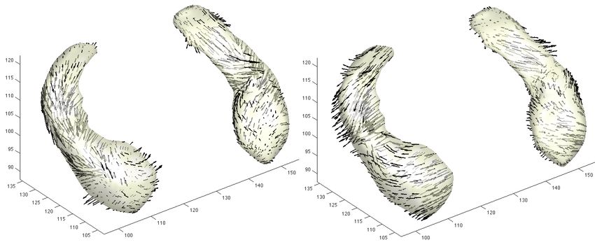
2 Chung
on anatomy (Sled et al. 1988). The next step is the tissue classification into three
types: gray matter, white matter and cerebrospinal fluid (CSF). This is critical
for identifying the tissue boundaries where surface measurements are obtained.
An artificial neural network classifier (Kollakian 1996, Ozkan et al. 1993) or
Gaussian mixture models (Good et al. 2001) can be used to segment the tissue
types automatically. The Statistical Parametric Mapping (SPM) package1 uses
a Gaussian mixture with a prior tissue density map.
After the segmentation, the tissue boundaries are extracted as triangular
meshes. In order to triangulate the boundaries, the marching cubes algorithm
(Lorensen & Cline 1987), level set method (Sethian 2002), the deformable sur-
faces method (Davatzikos & Bryan 1995) or anatomic segmentation using prox-
imities (ASP) method (MacDonald et al. 2000) can be used. Brain substructures
such as the brain stem and the cerebellum are usually automatically removed
in the process. The resulting triangular mesh is expected to be topologically
equivalent to a sphere. For example, the triangular mesh resulted from the ASP
method consists of 40,962 vertices and 81,920 triangles with the average intern-
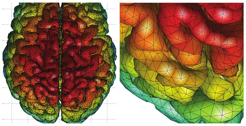
odal distance of 3 mm. Figure 1 shows a representative cortical mesh obtained
from ASP. Surface measurements such as cortical thickness can be automatically
obtained at each mesh vertex. Subcortical brain surfaces such as amygdala and
hippocampus are extracted similarly, but often done in a semi-automatic fash-
ion with the marching cubes algorithm on manual edited subcortical volumes.
In the hippocampus case study, the left and right hippocampi were manually
segmented in the template using the protocol outlined in (Rusch et al. 2001).
Fig. 1: Left: The outer cortical brain surface mesh consisting of 81,920 triangles.
Measurements are defined at mesh vertices. Right: The part of the mesh is
enlarged to show the convoluted nature of the surface.
1
The SPM package is available at www.fil.ion.ucl.ac.uk/spm.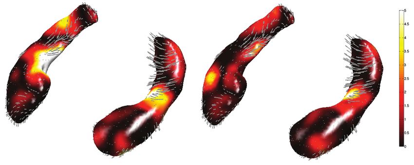
Statistical Analysis on Brain Surfaces       3

    Comparing measurements defined across different cortical surfaces is not triv-
ial due to the fact that no two cortical surfaces are identically shaped. In com-
paring measurements across different 3D whole brain images, 3D volume-based
image registration such as Advanced Normalization Tools (ANTS) (Avants et al.
2008) is needed. However, 3D image registration techniques tend to misalign sul-
cal and gyral folding patterns of the cortex. Hence, 2D surface-based registration
is needed in order to match measurements across different cortical surfaces. Var-
ious surface registration methods have been proposed (Chung et al. 2005, Chung
2012, Thompson & Toga 1996, Davatzikos 1997, Miller et al. 1997, Fischl et al.
1999). Most methods solve a complicated optimization problem of minimizing
the measure of discrepancy between two surfaces. A much simpler spherical har-
monic representation technique provide a simple way of approximately matching
surfaces without time-consuming numerical optimization (Chung 2012).
    Surface registration and the subsequent surface-based analysis usually require
parameterizing surfaces. It is natural to assume the surface mesh to be a discrete
approximation to the underlying cortical surface, which can be treated as a
smooth 2D Riemannian manifold. Cortical surface parameterization has been
done previously in (Thompson & Toga 1996, Joshi et al. 1995, Chung 2012).
The surface parameterization also provides surface shape features such as the
Gaussian and mean curvatures, which measure anatomical variations associated
with the deformation of the cortical surface during, for instance, development
and aging (Dale & Fischl 1999, Griffin 1994, Joshi et al. 1995, Chung 2012).

2   Surface Parameterization
In order to perform statistical analysis on a surface, parameterization of the
surface is often required (Chung 2012). Brain surfaces are often mapped onto
a plane or a sphere. Then surface measurements defined on mesh vertices are
also mapped onto the new domain and analyzed. However, almost all surface
parameterizations suffer metric distortions, which in turn influence the spatial
covariance structure so it is not necessarily the best approach.
    We model the cortical surface M as a smooth 2D Riemannian manifold
parameterized by two parameters u1 and u2 such that any point x ∈ M can be
represented as

      X(u1 , u2 ) = {x1 (u1 , u2 ), x2 (u1 , u2 ), x3 (u1 , u2 ) : (u1 , u2 ) ∈ D ⊂ R2 }

for some parameter space u = (u1 , u2 ) ∈ D ⊂ R2 (Boothby 1986, do Carmo
1992, Chung et al. 2003, Kreyszig 1959). The aim of the parameterization is
estimating the coordinate functions x1 , x2 , x3 as smoothly as possible.
    Both global and local parameterizations are available. A global parameteri-
zation, such as tensor B-splines and spherical harmonic representation, are com-
putationally expensive compared to a local surface parameterization. A local
surface parameterization in the neighborhood of point x = (x1 , x2 , x3 ) can be
obtained via the projection of the local surface patch onto the tangent plane
Tx (M) (Chung 2012, Joshi et al. 1995).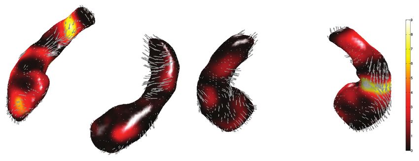
4     Chung

2.1   Local Parameterization by Quadratic Polynomial

A local parameterization is usually done by fitting a quadratic polynomial of the
form

              X(u1 , u2 ) = β1 u1 + β2 u2 + β3 (u1 )2 + β4 u1 u2 + β5 (u2 )2   (1)

in (u1 , u2 ) ∈ D ⊂ R2 . The data can be centered so there is no constant term in
the quadratic form (1) (Chung 2012). The coefficients βi are usually estimated
by the least squares method (Joshi et al. 1995, Khaneja et al. 1998, Chung 2012).
    In estimating various differential geometric measures such as the Laplace-
Beltrami operator or curvatures, it is not necessary to find global surface pa-
rameterization of M. Local surface parameterization such as the quadratic poly-
nomial fit is sufficient to obtain such geometric quantities (Chung 2012). The
drawback of the polynomial parameterization is that there is a tendency to weave
the outermost mesh vertices to find vertices in the center. Therefore this is not
advisable to directly fit (1) when one of the coordinate values rapidly changes.

2.2   Surface Flattening

Parameterizing cortical and subcortical surfaces with respect to simpler algebraic
surfaces such as a unit sphere is needed to establish a standard coordinate sys-
tem. However, polynomial regression type of local parameterization is ill-suited
for this purpose. For the global surface parameterization, we can use surface flat-
tening (Andrade et al. 2001, Angenent et al. 1999), which is nonparametric in
nature. The surface flattening parametrizes a surface by either solving a partial
differential equation or optimizing its variational form.
    Deformable surface algorithms naturally provide one-to-one maps from corti-
cal surfaces to a sphere since the algorithm initially starts with a spherical mesh
and deforms it to match the tissue boundaries (MacDonald et al. 2000). The
deformable surface algorithms usually start with the second level of triangular
subdivision of an icosahedron as the initial surface. After several iterations of
deformation and triangular subdivision, the resulting cortical surface contains
very dense triangle elements. There are many surface flattening techniques such
as conformal mapping (Angenent et al. 1999, Gu et al. 2004, Hurdal & Stephen-
son 2004) quasi-isometric mapping (Timsari & Leahy 2000), area preserving
mapping (Brechbuhler et al. 1995), and the Laplace equation method (Chung
2012).
    For many surface flattening methods to work, the starting binary object has
to be close to star-shape or convex. For shapes with a more complex struc-
ture, the methods may create numerical singularities in mapping to the sphere.
Surface flattening can destroy the inherent geometrical structure of the cortical
surface due to the metric distortion. Any structural or functional analysis associ-
ated with the cortex can be performed without surface flattening if the intrinsic
geometric method is used (Chung 2012).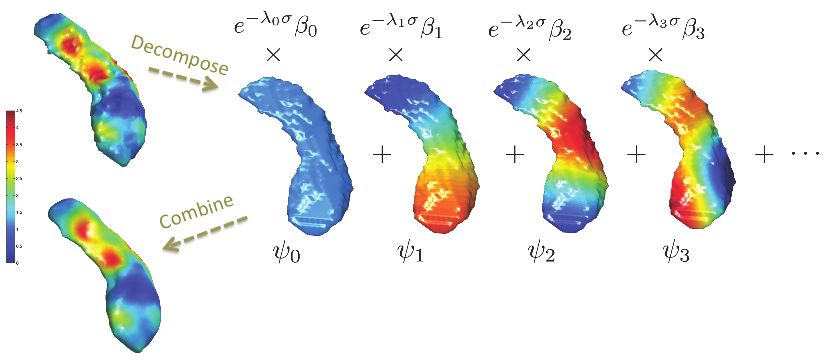
Statistical Analysis on Brain Surfaces    5

2.3    Spherical Harmonic Representation

The spherical harmonic (SPHARM) representation 2 is a widely used subcorti-
cal surface parameterization technique (Chung et al. 2008, Chung 2012, Gerig
et al. 2001, Gu et al. 2004, Kelemen et al. 1999, Shen et al. 2004). SPHARM
represents the coordinates of mesh vertices as a linear combination of spheri-
cal harmonics. SPHARM has been mainly used as a data reduction technique
for compressing global shape features into a small number of coefficients. The
main global geometric features are encoded in low degree coefficients while the
noise are in high degree spherical harmonics (Gu et al. 2004). The method has
been used to model various subcortical structures such as ventricles (Gerig et al.
2001), hippocampi (Shen et al. 2004) and cortical surfaces (Chung et al. 2008).
The spherical harmonics have a global support. So the resulting spherical har-
monic coefficients contain the global shape features and it is not possible to
directly obtain local shape information from the coefficients only. However, it is
still possible to obtain local shape information by evaluating the representation
at each fixed vertex, which gives the smoothed version of the coordinates of sur-
faces. In this fashion, SPHARM can be viewed as mesh smoothing (Chung et al.
2008, n.d.). In this section, we present a brief introduction of SPHARM within
a Hilbert space framework.
     Suppose there is a bijective mapping between the cortical surface M and a
unit sphere S 2 obtained through a deformable surface algorithm (Chung 2012).
Consider the parameterization of S 2 by

                      X(θ, ϕ) = (sin θ cos ϕ, sin θ sin ϕ, cos θ),

with (θ, ϕ) ∈ [0, π) ⊗ [0, 2π). The polar angle θ is the angle from the north pole
and the azimuthal angle ϕ is the angle along the horizontal cross-section. Using
the bijective mapping, we can parameterize functional data f with respect to
the spherical coordinates

                            f (θ, ϕ) = g(θ, ϕ) + (θ, ϕ),                           (2)

where g is a unknown smooth coordinate function and  is a zero mean random
field, possibly Gaussian. The error function  accounts for possible mapping
errors. The unknown signal g is then estimated in the finite subspace of L2 (S 2 ),
the space of square integrable functions in S 2 , spanned by spherical harmonics
in the least squares fashion (Chung et al. 2008).
    Previous imaging and shape modeling literature have used the complex-
valued spherical harmonics (Bulow 2004, Gerig et al. 2001, Gu et al. 2004, Shen
et al. 2004). In practice, however, it is sufficient to use only real-valued spherical
harmonics (Courant & Hilbert 1953, Homeier & Steinborn 1996), which is more
convenient in setting up a real-valued stochastic model (2). The relationship be-
tween the real- and complex-valued spherical harmonics is given in (Blanco et al.
2
    The SPHARM package is available at
    www.stat.wisc.edu/∼mchung/softwares/weighted-SPHARM/weighted-SPHARM.html
6 Chung
1997, Homeier & Steinborn 1996). The complex-valued spherical harmonics can
be transformed into real-valued spherical harmonics using an unitary transform.
The spherical harmonic Ylm of degree l and order m is defined as
|m|
clm Pl (cos θ) sin(|m|ϕ), −l ≤ m ≤ −1,
|m|
Ylm = c√lm2 Pl (cos θ), m = 0,
|m|
clm Pl (cos θ) cos(|m|ϕ), 1 ≤ m ≤ l,
q
2l+1 (l−|m|)! m
where clm = 2π (l+|m|)! and Pl is the associated Legendre polynomial of
order m (Courant & Hilbert 1953, Wahba 1990), which is given by
(1 − x2 )m/2 dl+m 2
Plm (x) = (x − 1)l , x ∈ [−1, 1].
2l l! dxl+m
The first few terms of the spherical harmonics are
r
1 3
Y00 = √ , Y1,−1 = sin θ sin ϕ,
4π 4π
r r
3 3
Y1,0 = cos θ, Y1,1 = sin θ cos ϕ.
4π 4π
The spherical harmonics are orthonormal with respect to the inner product
Z
hf1 , f2 i = f1 (Ω)f2 (Ω) dµ(Ω),
S2
where Ω = (θ, ϕ) and the Lebesgue measure dµ(Ω) = sin θdθdϕ. The norm is
then defined as
||f1 || = hf1 , f1 i1/2 . (3)
The unknown mean function g is estimated by minimizing the integral of
the squared residual in Hk , the space spanned by up to k-th degree spherical
harmonics:
Z 2
gb(Ω) = arg min f (Ω) − h(Ω) dµ(Ω). (4)
h∈Hk S2
It can be shown that the minimization is given by
k
X l
X
gb(Ω) = hf, Ylm iYlm (Ω), (5)
l=0 m=−l
the Fourier series expansion. The expansion (5) has been referred to as the
spherical harmonic representation (Chung et al. 2008, Gerig et al. 2001, Gu
et al. 2004, Shen et al. 2004, Shen & Chung 2006). This technique has been
used in representing various brain subcortical structures such as hippocampiStatistical Analysis on Brain Surfaces 7
Shen et al. (2004) and ventricles (Gerig et al. 2001) as well as the whole brain
cortical surfaces (Chung et al. 2008, Gu et al. 2004). By taking each component of
Cartesian coordinates of mesh vertices as the functional signal f , surface meshes
can be parameterized as a function of θ and ϕ.
The spherical harmonic coefficients can be estimated in least squares fash-
ion. However, for an extremely large number of vertices and expansions, the least
squares method may be difficult to directly invert large matrices. Instead, the
iterative residual fitting (IRF) algorithm (Chung et al. 2008) can be used to iter-
atively estimate the coefficients by partitioning the larger problem into smaller
subproblems. The IRF algorithm is similar to the matching pursuit method (Mal-
lat & Zhang 1993). The IRF algorithm was developed to avoid the computational
burden of inverting a large linear problem while the matching pursuit method
was originally developed to compactly decompose a time-frequency signal into a
linear combination of a pre-selected pool of basis functions. Although increasing
the degree of the representation increases the goodness-of-fit, it also increases
the number of estimated coefficients quadratically. So it is necessary to stop the
iteration at the specific degree k, where the goodness-of-fit and the number of
coefficients balance out. This idea was used in determining the optimal degree
of SPHARM (Chung et al. 2008).
The limitation of SPHARM is that it produces the Gibbs phenomenon, i.e.,
ringing artifacts, for discontinuous and rapidly changing continuous measure-
ments (Chung et al. 2008, Gelb 1997). The Gibbs phenomenon can be effec-
tively removed by weighting the spherical harmonic coefficients exponentially
smaller, which makes the representation smooth out rapidly changing signals.
The weighted version of SPHARM is related to isotropic diffusion smoothing
(Andrade et al. 2001, Cachia, Mangin, Riviére, Kherif, Boddaert, Andrade,
Papadopoulos-Orfanos, Poline, Bloch, Zilbovicius, Sonigo, Brunelle & Régis 2003,
Chung 2012, Chung et al. 2005) as well as the diffusion wavelet transform (Chung
et al. 2008, n.d., Hosseinbor et al. 2014).
3 Surface Registration
To construct a test statistic locally at each vertex across different surfaces, one
must register the surfaces to a common template surface. Nonlinear cortical
surface registration is often performed by minimizing objective functions that
measure the global fit of two surfaces while maximizing the smoothness of the
deformation in such a way that the cortical gyral or sulcal patterns are matched
smoothly (Chung et al. 2005, Robbins 2003, Thompson & Toga 1996). There
is also a much simpler way of aligning surfaces using SPHARM representation
(Chung et al. 2008). Before any sort of nonlinear registration is performed, an
affine registration is performed to align and orient the global brain shapes.
3.1 Affine Registration
Anatomical objects extracted from 3D medical images are aligned using affine
transformations to remove the global size differences. Affine registration requires8 Chung
identifying corresponding landmarks either manually or automatically. The affine
transform T of point p = (p1 , · · · , pd )0 ∈ Rd to q = (q1 , · · · , qd )0 is given by
q = Rp + c,
where the matrix R corresponds to rotation, scaling and shear while c corre-
sponds to translation. Although the affine transform is not linear, it can be
made into a linear form by augmenting the transform. The affine transform can
be rewritten as
q R c p
= . (6)
1 0···0 1 1
Let
R c
A= .
0···0 1
Trivially, A is linear a linear operator. The matrix A is the most often used form
for recording the affine registration.
Let pi be the i-th landmark and its corresponding affine transformed points
qi . Then we rewrite (6) as
p1 · · · pn
q1 · · · qn = R c .
| {z } 1 ··· 1
Q | {z }
P
Then the least squares estimation is given as
R
bbc = QP 0 (P P 0 )−1 .
Then the points pi are mapped to Rpb i+b c, which may not coincide with qi in
general. In practice, landmarks are automatically identified from T1-weighted
MRI.
3.2 SPHARM Correspondence
Using SPHARM, it is possible to approximately register surfaces with different
mesh topology without any optimization. The crude alignment can be done by
coinciding the first order ellipsoid meridian and equator in the SPHARM repre-
sentation (Gerig et al. 2001, Styner et al. 2006). However, this can be improved.
Consider SPHARM representation of surface H = (h1 , h2 , h3 ) with spherical
angles Ω given by
Xk Xl
hi (Ω) = hilm Ylm (Ω),
l=0 m=−l
where (v1 , v2 , v3 ) are the coordinates of mesh vertices and SPHARM coefficient
hilm = hvi , Ylm i. Consider another SPHARM representation J = (j1 , j2 , j3 ) ob-
tained from mesh coordinate wi :
k
X l
X
i
ji (Ω) = wlm Ylm (Ω),
l=0 m=−lStatistical Analysis on Brain Surfaces 9
i
where wlm = hwi , Ylm i. Suppose the surface hi is deformed to hi + di by the
amount of displacement di . We wish to find di that minimizes the discrepancy
between hi + di and ji in the subspace Hk spanned using up to the k-th degree
spherical harmonics. It can be shown that
k
X l
X
i i
arg min hbi + di − jbi = (wlm − vlm )Ylm (Ω). (7)
di ∈Hk
l=0 m=−l
This implies that the optimal displacement of matching two surfaces is obtained
by simply taking the difference between two SPHARM and matching coefficients
of the same degree and order. Then a specific point hbi (Ω) in one surface cor-
responds to jbi (Ω) in the other surface. We refer to this point-to-point surface
matching as the SPHARM correspondence (Chung et al. 2008). Unlike other
surface registration methods (Chung et al. 2005, Robbins 2003, Thompson &
Toga 1996), it is not necessary to consider an additional cost function that
guarantees the smoothness of the displacement field since the displacement field
d = (d1 , d2 , d3 ) is already a linear combination of smooth basis functions.
Fig. 2: The displacement vector fields of registering from the hippocampus tem-
plate to two individual surfaces. The displacement vector field is obtained from
the diffeomorphic image registration (Avants et al. 2008). The variability in the
displacement vector field can be analyzed using a multivariate general linear
model (Chung 2012).
3.3 Diffeomorphic Registration
Diffeomorphic image registration is a recently popular technique for registering
volume and surface data (Avants et al. 2008, Miller & Qiu 2009, Vaillant et al.
2007, Qiu & Miller 2008, Yang et al. 2011). From the affine transformed indi-
vidual surfaces Mj , an additional nonlinear surface registration to the template10 Chung
using the large deformation diffeomorphic metric mapping (LDDMM) frame-
work can be performed (Miller & Qiu 2009, Vaillant et al. 2007, Qiu & Miller
2008, Yang et al. 2011). In LDDMM, given the template surface M, the dif-
feomorphic transformations, which are one-to-one, smooth forward, and inverse
transformation, are constructed as follows. We estimate the diffeomorphism d
between them as a smooth streamline given by the Lagrangian evolution:
∂d
(x, t) = v ◦ d(x, t)
∂t
with d(x, 0) = x, t ∈ [0, 1] for time-dependent velocity field v. Note the surfaces
Mj and M are the start and end points of the diffeomorphism, i.e. Mj ◦d(·, 0) =
Mj and Mj ◦ d(·, 1) = M. By solving the evolution equation numerically, we
obtain the diffeomorphism. By averaging the inverse deformation fields from the
template M to individual subjects, we may obtain yet another final more refined
template. The vector fields v are constrained to be sufficiently smooth to generate
diffeomorphic transformations over finite time (Dupuis et al. 1998). Figure 2
shows the resulting displacement vector fields of warping from the template to
two hippocampal surfaces. In the deformation-based morphometry, variability in
the displacement is used to characterize surface growth and differences (Chung
2012).
4 Cortical Surface Features
The human cerebral cortex has the topology of a 2D highly convoluted grey
matter shell with an average thickness of 3 mm (Chung 2012, MacDonald et al.
2000). The outer boundary of the shell is called the outer cortical surface while
the inner boundary is called the inner cortical surface. Various cortical surface
features such as curvatures, local surface area and cortical thickness have been
used in quantifying anatomical variations. Among them, cortical thickness has
been more often analyzed than other features.
4.1 Cortical Thickness
Once we extract both the outer and inner cortical surface meshes, cortical thick-
ness can be computed at each mesh vertex. The cortical thickness is defined as
the distance between the corresponding vertices between the inner and outer
surfaces (MacDonald et al. 2000). There are many different computational ap-
proaches in measuring cortical thickness. In one approach, the vertices on the
inner triangular mesh are deformed to fit the outer surface by minimizing a cost
function that involves bending, stretch and other topological constraints (Chung
2012). There is also an alternate method for automatically measuring cortical
thickness based on the Laplace equation (Jones et al. 2000).
The average cortical thickness for each individual is about 3 mm (Henery
& Mayhew 1989). Cortical thickness varies from 1 to 4 mm depending on the
location of the cortex. In normal brain development, it is highly likely thatStatistical Analysis on Brain Surfaces 11
the change of cortical thickness may not be uniform across the cortex. Since
different clinical populations are expected to show different patterns of cortical
thickness variations, cortical thickness has also been used as a quantitative index
for characterizing a clinical population (Chung et al. 2005). Cortical thickness
varies locally by region and is likely to be influenced by aging, development and
disease (Barta et al. 2005). By analyzing how cortical thickness varies between
clinical and non-clinical populations, we can locate regions on the brain related
to a specific pathology.
4.2 Surface Area and Curvatures
As in the case of local volume changes in the deformation-based morphometry,
the rate of cortical surface area expansion or reduction may not be uniform
across the cortical surface (Chung 2012). Suppose that cortical surface M is
parameterized by the parameters u = (u1 , u2 ) such that any point x ∈ M can
be written as x = X(u). Let Xi = ∂X/∂ui be the partial derivative vectors.
The Riemannian metric tensor gij is then given by the inner product between
two vectors Xi and Xj , i.e.
gij (t) = hXi , Xj i.
The tensor gij measures the amount of the deviation of the cortical surface from
a flat Euclidean plane and can be used to measure lengths, angles and areas on
the cortical surface.
Let g = (gij ) be a 2 × 2 matrix of metric tensors. The total surface area of
the cortex M is then given by
Z p
det g du,
D
√
where D = X −1 (M) is the parameter space (Kreyszig 1959). The term det g
is called the surface area element and it measures the transformed area of the
unit square in the parameter space D via transformation X : D → M. The
surface area element can be considered as the generalization of the Jacobian
determinant, which is used in measuring local volume changes in the tensor-
based morphometry (Chung 2012).
Instead of using the metric tensor formulation, it is possible to quantify
local surface area change in terms of the areas of the corresponding triangles in
surface meshes. However, this formulation assigns the computed surface area to
each face instead of each vertex. This causes a problem in both surface-based
smoothing and statistical analysis, where values are required to be given on
vertices. Interpolating scalar values on vertices from face values can be done
by the weighted average of face values. It is not hard to develop surface-based
smoothing and statistical analysis on face values, as a form of dual formulation,
but the cortical thickness and the curvature metric are defined on vertices so we
end up with two separate approaches: one for metrics defined on vertices and
the other for metrics defined on faces. Therefore, the metric tensor approach12 Chung
provides a better unified quantitative framework for the subsequent statistical
analysis.
The principal curvatures characterize the shape and location of the sulci and
gyri, which are the valleys and crests of the cortical surfaces (Bartesaghi & Sapiro
2001, Joshi et al. 1995, Khaneja et al. 1998). By measuring the curvature changes,
rapidly folding and cortical regions can be localized. The principal curvatures κ1
and κ2 can be represented as functions of βi in quadratic surface (1) (Boothby
1986, Kreyszig 1959).
4.3 Gray Matter Volume
Local volume can be computed using the determinant of the Jacobian of de-
formation and used in detecting the regions of brain tissue growth and loss in
brain development (Chung 2012). Compared to the local surface area change,
the local volume change measurement is more sensitive to small deformation of
the brain. If a unit cube increases its sides by one, the surface area will increase
by 22 − 1 = 3 while the volume will increase by 23 − 1 = 7. Therefore, the statis-
tical analysis based on the local volume change is at least twice more sensitive
compared to that of the local surface area change. So the local volume change
should be able to pick out gray matter tissue growth patterns even when the
local surface area change may not.
The gray matter can be considered as a thin shell bounded by two sur-
faces with varying cortical thickness. In most deformable surface algorithms like
FreeSurfer, each triangle on the outer surface has a corresponding triangle on
the inner surface. Let p1 , p2 , p3 be the three vertices of a triangle on the outer
surface and q1 , q2 , q3 be the corresponding three vertices on the inner surface
such that pi is linked to qi . Then the volume of the triangular prism is given by
the sum of the determinants
D(p1 , p2 , p3 , q1 ) + D(p2 , p3 , q1 , q2 ) + D(p3 , q1 , q2 , q3 )
where
D(a, b, c, d) = | det(a − d, b − d, c − d)|/6
is the volume of a tetrahedron whose vertices are {a, b, c, d}. Afterwards, the
total gray matter volume can be estimated by summing the volumes of all tri-
angular prisms (Chung 2012).
5 Surface Data Smoothing
Cortical surface mesh extraction and cortical thickness computation are expected
to introduce noise (Chung et al. 2005, Fischl & Dale 2000, MacDonald et al.
2000). To counteract this, surface-based data smoothing is necessary (Andrade
et al. 2001, Cachia, Mangin, Riviére, Papadopoulos-Orfanos, Kherif, Bloch &
Régis 2003, Cachia, Mangin, Riviére, Kherif, Boddaert, Andrade, Papadopoulos-
Orfanos, Poline, Bloch, Zilbovicius, Sonigo, Brunelle & Régis 2003, Chung 2012).Statistical Analysis on Brain Surfaces 13
For 3D whole brain volume data, Gaussian kernel smoothing is desirable in
many statistical analyses (Dougherty 1999, Rosenfeld & Kak 1982). Gaussian
kernel smoothing weights neighboring observations according to their 3D Eu-
clidean distance. Specifically, Gaussian kernel smoothing of functional data or
image f (x),√ x = (x1 , . . . , xn ) ∈ Rn with full width at half maximum (FWHM)
1/2
= 4(ln 2) t is defined as the convolution of the Gaussian kernel with f :
Z
1 2
F (x, t) = n/2
e−(x−y) /4t f (y)dy. (8)
(4πt) Rn
However, due to the convoluted nature of the cortex, whose geometry is non-
Euclidean, we cannot directly use the formulation (8) on the cortical surface.
For data that lie on a 2D surface, smoothing must be weighted according to the
geodesic distance along the surface, which is not straightforward (Andrade et al.
2001, Chung 2012, Chung et al. 2001).
5.1 Diffusion Smoothing
By formulating Gaussian kernel smoothing as a solution of a diffusion equation
on a Riemannian manifold, the Gaussian kernel smoothing approach can be
generalized to an arbitrary curved surface. This generalization is called diffusion
smoothing and was first introduced in the analysis of fMRI data on the cortical
surface (Andrade et al. 2001) and cortical thickness (Chung et al. 2001) in 2001.
It can be shown that Gaussian kernel smoothing (8) is the integral solution
of the n-dimensional diffusion equation
∂F
= ∆F (9)
∂t
with the initial condition F (x, 0) = f (x), where
∂2 ∂2
∆= + · · · +
∂x21 ∂x2n
is the Laplacian in n-dimensional Euclidean space. Hence the Gaussian kernel
smoothing is equivalent to the diffusion of the initial data f (x) after time t.
Diffusion equations have been widely used in image processing as a form of
noise reduction starting with Perona and Malik in 1990 (Perona & Malik 1990).
Numerous diffusion techniques have been developed for surface data smoothing
(Andrade et al. 2001, Chung 2012, Cachia, Mangin, Riviére, Kherif, Boddaert,
Andrade, Papadopoulos-Orfanos, Poline, Bloch, Zilbovicius, Sonigo, Brunelle
& Régis 2003, Cachia, Mangin, Riviére, Papadopoulos-Orfanos, Kherif, Bloch
& Régis 2003, Chung et al. 2005, Joshi et al. 2009). When applying diffusion
smoothing on curved surfaces, the smoothing somehow has to incorporate the
geometrical features of the curved surface and the Laplacian ∆ should change ac-
cordingly. The extension of the Euclidean Laplacian to an arbitrary Riemannian
manifold is called the Laplace-Beltrami operator (Arfken 2000, Kreyszig 1959).14 Chung
The approach taken in (Andrade et al. 2001) is based on a local flattening of
the cortical surface and estimating the planar Laplacian, which may not be as
accurate as the cotan estimation based on the finite element method (FEM)
given in (Chung et al. 2001). Further, the FEM approach completely avoids the
use of surface flattening and parameterization; thus, it is more robust.
For given Riemannian metric tensor gij , the Laplace-Beltrami operator ∆ is
defined as
X 1 ∂ 1/2 ij ∂F
∆F = |g| g , (10)
i,j
|g|1/2 ∂ui ∂uj
where (g ij ) = g −1 (Arfken 2000). Note that when g becomes an identity matrix,
the Laplace-Beltrami operator reduces to the standard 2D Laplacian:
∂2F ∂2F
∆F = + .
∂(u1 )2 ∂(u2 )2
Using FEM on the triangular cortical mesh, it is possible to estimate the Laplace-
Beltrami operator as the linear weights of neighboring vertices using the cotan
formulation, which is first given in (Chung et al. 2001).
Fig. 3: A typical triangulation in the neighborhood of p = p0 in a surface mesh.
Let p1 , · · · , pm be m neighboring vertices around the central vertex p = p0
(Figure 3). Then the estimated Laplace-Beltrami operator is given by
m
X
∆F
d (p) = wi F (pi ) − F (p) (11)
i=1
with the weights
cot θi + cot φi
wi = Pm ,
i=1 kTi kStatistical Analysis on Brain Surfaces 15
where θi and φi are the two angles opposite to the edge connecting pi and p,
and kTi k is the area of the i-th triangle (Figure 3).
FEM estimation (11) is an improved formulation from the previous attempt
in diffusion smoothing (Andrade et al. 2001), where the Laplacian is simply
estimated as the planar Laplacian after locally flattening the triangular mesh
consisting of nodes p0 , · · · , pm onto a flat plane. Afterwards, the finite difference
(FD) scheme can be used to iteratively solve the diffusion equation at each vertex
p:
F (p, tn+1 ) − F (p, tn )
= ∆F
b (p, tn ),
tn+1 − tn
with the initial condition F (p, 0) = f (p) and fixed δt = tn+1 − tn . After N
iterations, the FD gives the diffusion of the initial data f after time N δt. If the
diffusion were applied to Euclidean space, it would be approximately equivalent
to Gaussian kernel smoothing with
√
FWHM = 4(ln 2)1/2 N δt.
For large meshes, computing the linear weights for the Laplace-Beltrami operator
takes a fair amount of time, but once the weights are computed, it is applied
repeatedly throughout the iterations as a matrix multiplication. Unlike Gaussian
kernel smoothing, diffusion smoothing is an iterative procedure.
5.2 Iterated Kernel Smoothing
Diffusion smoothing use FEM and FD, which are known to suffer numerical
instability if sufficiently small step size is not chosen in the forward Euler scheme.
To remedy the problem associated with diffusion smoothing, iterative kernel
smoothing3 was introduced (Chung et al. 2005). The method has been used in
smoothing various cortical surface data: cortical curvatures (Luders, Thompson,
Narr, Toga, Jancke & Gaser 2006, Gaser et al. 2006), cortical thickness (Luders,
Narr, Thompson, Rex, Woods, DeLuca, Jancke & Toga 2006, Bernal-Rusiel et al.
2008), hippocampus (Shen et al. 2006, Zhu et al. 2007), magnetoencephalography
(MEG) (Han et al. 2007) and functional-MRI (Hagler Jr. et al. 2006, Jo et al.
2007). This and its variations are probably the most widely used method for
smoothing brain surface data at this moment. In iterated kernel smoothing,
kernel weights are spatially adapted to follow the shape of the heat kernel in a
discrete fashion.
The n-th iterated kernel smoothing of signal f ∈ L2 (M) with kernel Kσ is
defined as
Kσ(n) ∗ f (p) = Kσ ∗ · · · ∗ Kσ ∗f (p),
| {z }
n times
where σ is the bandwidth of the kernel. If Kσ is a heat kernel, we have the
following iterative relation (Chung et al. 2005):
(n)
Kσ ∗ f (p) = Kσ/n ∗ f (p). (12)
3
MATLAB package: www.stat.wisc.edu/∼mchung/softwares/hk/hk.html.16 Chung
The relation (12) shows that kernel smoothing with large bandwidth σ can be
decomposed into n repeated applications of kernel smoothing with smaller band-
width σ/n. This idea can be used to approximate the heat kernel. When the
bandwidth is small, the heat kernel behaves like the Dirac-delta function and,
using the parametrix expansion (Rosenberg 1997, Wang 1997), we can approxi-
mate it locally using the Gaussian kernel.
Let p1 , · · · , pm be m neighboring vertices of vertex p = p0 in the mesh. The
geodesic distance d(p, p0 ) between p and its adjacent vertex pi is the length of
edge between these two vertices in the mesh. Then the discretized and normalized
heat kernel is given by
d(p,pi )2
exp − 4σ
Wσ (p, pi ) = Pm d(p−pj )2
.
j=0 exp − 4σ
Pm
Note i=0 Wσ (p, pi ) = 1. For small bandwidth, all the kernel weights are con-
centrated near the center, so we only need to worry about the first neighbors of
a given vertex in a surface mesh. The discrete version of heat kernel smoothing
on a triangle mesh is then given by
m
X
Wσ ∗ f (p) = Wσ (p, pi )f (pi ).
i=0
The discrete kernel smoothing should converge to heat kernel smoothing as the
mesh resolution increases. This is the form of the Nadaraya-Watson estimator
(Chaudhuri & Marron 2000) in statistics. Instead of performing a single kernel
smoothing with large bandwidth nσ, we perform n iterated kernel smoothing
(n)
with small bandwidth σ as follows Wσ ∗ f (p).
5.3 Heat Kernel Smoothing
The recently proposed heat kernel smoothing4 framework constructs the heat
kernel analytically using the eigenfunctions of the Laplace-Beltrami operator
(Seo et al. 2010). This method avoids the need for the linear approximation used
in iterative kernel smoothing that compounds the approximation error at each
iteration. The method represents isotropic heat diffusion analytically as a series
expansion so it avoids the numerical convergence issues associated with solving
the diffusion equations numerically (Andrade et al. 2001, Chung 2012, Joshi et al.
2009). This technique is different from other diffusion-based smoothing methods
in that it bypasses the various numerical problems such as numerical instability,
slow convergence, and accumulated linearization error.
Although recently there have been a few studies that introduce heat kernel
in computer vision and machine learning (Belkin et al. 2006), they mainly use
heat kernel to compute shape descriptors (Sun et al. 2009, Bronstein & Kokkinos
2010) or to define a multi-scale metric (de Goes et al. 2008). These studies did not
4
MATLAB package: brainimaging.waisman.wisc.edu/∼chung/lb.Statistical Analysis on Brain Surfaces 17
use heat kernel in smoothing functional data on manifolds. Further, most kernel
methods in machine learning deal with the linear combination of kernels as a
solution to penalized regressions, which significantly differs from the heat kernel
smoothing framework, which does not have a penalized cost function. There are
log-Euclidean and exponential map frameworks on manifolds, where the main
interest is in computing the Fréchet mean along the tangent space (Davis et al.
2010, Fletcher et al. 2004). Such approaches or related methods in (Gerber et al.
2009), the Nadaya-Watson type of kernel regression is reformulated to learn the
shape or image means in a population. In the heat kernel smoothing framework,
we are not dealing with manifold data but scalar data defined on a manifold, so
there is no need for exploiting the manifold structure of the data itself.
Let ∆ be the Laplace-Beltrami operator on M. Solving the eigenvalue equa-
tion
∆ψj = −λψj , (13)
we order eigenvalues
0 = λ0 < λ1 ≤ λ2 ≤ · · · ,
and corresponding eigenfunctions ψ0 , ψ1 , ψ2 , · · · (Rosenberg 1997, Chung et al.
2005, Lévy 2006, Shi et al. 2009). The eigenfunctions ψj form an orthonormal
basis in L2 (M), the space of square integrable functions in M. Figure 4 shows
the first four LB-eigenfunctions on a hippocampal surface.
There is extensive literature on the use of eigenvalues and eigenfunctions of
the Laplace-Beltrami operator in medical imaging and computer vision (Lévy
2006, Qiu et al. 2006, Reuter et al. 2009, Reuter 2010, Zhang et al. 2007, 2010).
The eigenvalues have been used in caudate shape discriminators (Niethammer
et al. 2007). Qiu et al. used eigenfunctions in constructing splines on cortical
surfaces (Qiu et al. 2006). Reuter used the topological features of eigenfunctions
(Reuter 2010). Shi et al. used the Reeb graph of the second eigenfunction in
shape characterization and landmark detection in cortical and subcortical struc-
tures (Shi et al. 2008, 2009). Lai et al. used the critical points of the second
eigenfunction as anatomical landmarks for colon surfaces (Lai et al. 2010).
Using the eigenfunctions, heat kernel Kσ (p, q) is defined as
∞
X
Kσ (p, q) = e−λj σ ψj (p)ψj (q), (14)
j=0
where σ is the bandwidth of the kernel. The heat kernel is the generalization of
a Gaussian kernel. Then heat kernel smoothing of functional measurement Y is
defined as
X∞
Kσ ∗ Y (p) = e−λj σ βj ψj (p), (15)
j=0
where βj = hY, ψj i are Fourier coefficients (Chung et al. 2005). Kernel smoothing
Kσ ∗ Y is taken as the estimate for the unknown mean signal θ. The degree
for truncating the series expansion can be automatically determined using the18 Chung
Fig. 4: Schematic of hat kernel smoothing on a hippocampal surface. Given a
noisy functional data on the surface, the Laplace-Beltrami eigenfunctions ψj
are computed and their exponentially weighted Fourier coefficients exp −λj σ are
multiplied as a form a regression. This process smoothes out the noisy functional
signal with bandwidth σ.
forward model selection procedure (Chung et al. 2008). Figure 4 shows the heat
kernel smoothing results with the bandwidth σ = 0.5 and k = 500 number of
LB-eigenfunctions.
Unlike previous approaches to heat diffusion (Andrade et al. 2001, Chung
2012, Joshi et al. 2009, Tasdizen et al. 2006), heat kernel smoothing avoids the
direct numerical discretization of the diffusion equation. Instead, we discretize
the basis functions of given manifold M by solving for the eigensystem (13) and
obtain λj and ψj . This provides more robust stable smoothing results compared
to diffusion smoothing or iterated kernel smoothing approaches.
6 Statistical Inference on Surfaces
Surface measurements such as cortical thickness, curvatures, or fMRI responses
can be modeled as random fields on the cortical surface:
Y (x) = µ(x) + (x), x ∈ M, (16)
where the deterministic part µ is the unknown mean of the observed functional
measurement Y and is a mean zero random field. The functional measurements
on the brain surface is often modeled using the general linear models (GLMs) or
its multivariate version. Various statistical models are proposed for estimating
and modeling the signal component µ(x) (Joshi et al. 1995, Chung 2012, Chung
et al. 2008) but the majority of the methods are all based on GLM. GLMs
have been implemented in the brain image analysis packages such as SPM and
fMRISTAT5 .
5
The fMRISTAT package is available at www.math.mcgill.ca/keith/fmristat.Statistical Analysis on Brain Surfaces 19
6.1 General Linear Models
We set up a GLM at each mesh vertex. Let yi be the response variable, which
is mainly coming from images and xi = (xi1 , · · · , xip ) to be the variables of
interest and zi = (zi1 , · · · , zik ) to be nuisance variables corresponding to the
i-th subject. Assume there are n subjects, i.e., i = 1, · · · , n. We are interested in
testing the significance of variables xi while accounting for nuisance covariates
zi . Then we set up GLM
yi = zi λ + xi β + i
where λ = (λ1 , · · · , λk )0 and β = (β1 , · · · , βp )0 are unknown parameter vectors
to be estimated. We assume to be the usual zero mean Gaussian noise, although
the distributional assumption is not required for the least squares estimation.
We test hypotheses
H0 : β = 0 vs. H1 : β 6= 0.
Subsequently the inference is done by constructing the F -statistic with p and
n − p − k degrees of freedom. GLMs have been used in quantifying cortical
thickness, for instance, in child development (Chung 2012, Chung et al. 2005)
and amygdala shape differences in autism (Chung 2012).
In the hippocampus case study, the first T1-weighted MRI scans are taken at
11.6 ± 3.7 years for n = 124 children using a 3T GE SIGNA scanner. Variables
age and gender are available. We also have variable income, which is a binary
dummy variable indicating whether the subjects are from high- or low-income
families. A total of 124 children and adolescents are from high- (> 75000$;
n = 86) and low-income (< 35000$, n = 38) parents respectively. In addition to
this cross-sectional data, longitudinal data was available for 82 of these subjects
(n = 66, > 75000$; n = 16, < 35000$). The second MRI scan was acquired for
these 82 subjects about 2 years later at 14 ± 3.9 years. For now, we will simply
ignore the correlation between the scans within a subject and will treat them as
independent.
On the template surface, we have the displacement vector fields of mapping
from the template to individual subjects (Figure 2). We take the length of the
surface displacement, denoted as deformation, with respect to the template
as the response variable. The displacement measures the shape difference with
respect to the template. However, since the length measurement is noisy, surface-
based smoothing is necessary. We have used heat kernel smoothing to smooth
out noise with the bandwidth 1 and 500 LB-eigenfunctions. Then we set up the
GLM:
deformation = λ1 + λ2 age + β1 income +
and test for the significance of β1 at each mesh vertex. Figure 5-left shows the
F -statistic result on testing β1 .
6.2 Multivariate General Linear Models
The multivariate general linear models (MGLMs) have been also used in mod-
eling multivariate imaging features on brain surfaces. These models generalize20 Chung
Fig. 5: F -statistics maps on testing the significant hippocampus shape difference
on the income level while controlling for age and gender. The arrows show the
deformation differences between the groups (high income − low income). The
fixed-effects result (left) is obtained by treating the repeat scans as indepen-
dent. The mixed-effects result (right) is obtained by explicating modeling the
covariance structure of the repeat scans with a subject. Both results are not
statistically significant under multiple comparisons even at 0.1 level.
a widely used univariate GLM by incorporating vector valued responses and
explanatory variables (Anderson 1984, Friston et al. 1995, Worsley et al. 1996,
2004, Taylor & Worsley 2008, Chung 2012). Hotelling’s T 2 statistic is a special
case of MGLM that has been used primarily for inference on surface shapes,
deformations and multi-scale features (Cao & Worsley 1999, Chung 2012, Gaser
et al. 1999, Joshi 1998, Kim et al. 2012, Thompson et al. 1997). An example
of this approach is Hotelling’s T 2 -statistic applied in determining the 3D brain
morphology of HIV/AIDS patients (Lepore et al. 2006). Hotelling’s T 2 -statistic
is also applied to 2D deformation tensor at each mesh vertex on the hippocampal
surface as a way to characterize AlzheimerÕs diseases (Wang et al. 2011).
Suppose there are a total of n subjects and p multivariate features of inter-
est at each voxel. For MGLM to work, n should be significantly larger than p.
Let Jn×p = (Jij ) be the measurement matrix, where Jij is the measurement for
subject i and for the j-th feature. The subscripts denote the dimension of the
matrix. All the measurements over subjects for the j-th feature are denoted as
xj = (J1j , · · · , Jnj )0 . The measurement vector for the i-th subject is denoted as
yi = (Ji1 , · · · , Jip )0 . yi is expected to be distributed identically and indepen-
dently over subjects. Note that
J = (x1 , · · · , xp ) = (y1 , · · · , yn )0 .
We may assume the covariance matrix of yi to be
Cov(y1 ) = · · · = Cov(yn ) = Σp×p = (σkl ).Statistical Analysis on Brain Surfaces 21
With these notations, we now set up the following MGLM at each mesh vertex:
1/2
Jn×p = Xn×k Bk×p + Zn×q Gq×p + Un×p Σp×p . (17)
X is the matrix of contrasted explanatory variables while B is the matrix of
unknown coefficients. Nuisance covariates are in matrix Z and the corresponding
coefficients are in matrix G. The components of Gaussian random matrix U
are independently distributed with zero mean and unit variance. Symmetric
matrix Σ1/2 is the square root of the covariance matrix accounting for the spatial
dependency across different voxels. In MGLM (17), we are usually interested in
testing hypotheses
H0 : B = 0. vs. H1 : B 6= 0.
The parameter matrices in the model are estimated via the least squares method.
The multivariate test statistics such as Lawley-Hotelling trace or Roy’s maximum
root are used to test the significance of B. When there is only one voxel, i.e. p = 1,
these multivariate test statistics collapse to Hotelling’s T 2 statistic (Worsley
et al. 2004, Chung 2012).
6.3 Small-n Large-p Problems
GLM are usually fitted in each voxel separately. Instead of fitting GLM at each
voxel, one may be tempted to fit the model in the whole brain surface. For
FreeSurfer meshes, we need to fit GLM over 300000 vertices, which causes the
small-n large-p problem (Friston et al. 1995, Schäfer & Strimmer 2005, Chung
2013).
Let yj be the measurement vector at the j-th vertex. Assume there are n
subjects and total p vertices in the surface. We have the same design matrix Z
for all p vertices. Then we need to estimate the parameter vector λj in
yj = Zλj (18)
for each j. Instead of solving (18) separately at each vertex, we combine all of
them together so that we have matrix equation
[y1 , · · · , ym ] = Z [λ1 , · · · , λm ] . (19)
| {z } | {z }
Y Λ
The least squares estimation of the parameter matrix Λ is given by
b = (Z0 Z)−1 Z0 Y.
Λ
Note that Z is of size n by p and Z0 Z is only invertible when n
p. The least
squares estimation does not provide robust parameter estimates for n
p, which
is the usual case in surface modeling. For small-n large-p problem, GLM need
to be regularized using the L1-norm penalty (Banerjee et al. 2006, 2008, Chung
2013, Friedman et al. 2008, Huang et al. 2010, Mazumder & Hastie 2012).22 Chung
6.4 Longitudinal Models
So far we have only dealt with an imaging data set where the parameters of the
model are fixed and do not vary across subjects and scans. Such fixed-effects
models are inadequate in modeling the within-subject dependency in longitudi-
nally collected imaging data. However, mixed-effects models can explicitly model
such dependency (Fox 2002, Milliken & Edland 2000, Molenberghs & Verbeke
2005, Pinehiro & Bates 2002). There are three advantages of the mixed-effects
model over the usual fixed-effects model. It explicitly models individual growth
patterns and accommodates an unequal number of follow-up image scans per
subject and unequal time intervals between scans.
The longitudinal outcome Yi from the i-th subject is modeled using the
mixed-effects model (Milliken & Edland 2000) as
Yi = Xi β + Zi γi + ei , (20)
where β is the fixed-effects shared by all subjects. γi is the subject-specific
random-effects and ei ∼ N (0, σ 2 ) is independent and identically distributed
noise. Xi and Zi are the design matrices corresponding to the fixed and ran-
dom effects respectively for the i-th subject. We assume γi ∼ N (0, Γ ) and
i ∼ N (0, Σi ) with some covariance matrices Γ and Σi . Hierarchically we are
modeling (20) as
Yi |γi ∼ N (Xi β + Zi γi , Σi ), γi ∼ N (0, Γ ).
Γ accounts for covariance among random effect terms. The within-subject vari-
ability between the scans is expected to be smaller than between-subject vari-
ability and explicitly modeled by Σi . The covariance of γi and are expected to
have block diagonal structure such that there is no correlation among the scans
of different subjects while there is high correlation between the scans of the same
subject:
γi Γ 0
V = .
i 0 Σi
Subsequently, the overall covariance of Yi is given by
VYi = Zi Γ Zi0 + Σi .
The random-effect contribution is Zi Γ Zi0 while the within-subject contribution
is Σi .
The parameters and the covariance matrices can be estimated via the re-
stricted maximum likelihood (REML) method (Fox 2002, Pinehiro & Bates
2002). The most widely used tools for fitting the mixed-effects model are the
nlme library in the R statistical package (Pinehiro & Bates 2002). However,
there is no need to use R to fit the mixed-effects model. Keith Worsley has im-
plemented the REML procedure in the SurfStat package6 (Chung 2012, Worsley
et al. 2009).
6
The MATLAB package is available at www.math.mcgill.ca/keith/surfstat.Statistical Analysis on Brain Surfaces 23
Here we briefly explain how to set up a longitudinal mixed-effect model in
practice. In the usual fixed-effect model, we have a linear model containing the
fixed-effect term agei for the i-th subject:
yi = β0 + β1 agei + i , (21)
where i is assumed to follow independent Gaussian. In (21), every subject has
identical growth trajectory β0 + β1 age, which is unrealistic. Biologically, each
subject is expected to have its own unique growth trajectory. So we assume each
subject to have its own intercept β0 + γi0 and slope β1 + γi1 :
yi = β0 + γi0 + (β1 + γi1 )agei + i . (22)
It is reasonable to assume the random vector γ = (γi0 , γi1 ) to be multivariate
normal. The model (22) can be decomposed into fixed- and random-effect terms:
yi = (β0 + β1 agei ) + (γi0 + γi1 agei ) + i . (23)
The fixed-effect term β0 + β1 agei models the linear growth of the population
while the random-effect term γi0 + γi1 agei models the subject specific growth
variations. Incorporating additional factors and interaction terms are done sim-
ilarly.
Fig. 6: F -statistics maps on testing the interaction between the income level
and age while controlling for gender in a linear mixed-effects model. The arrows
show the deformation differences between the groups (high income - low income).
Significant regions are only found in the tail and midbody regions of the right
hippocampus.
In the hippocampus case study, the first MRI scans are taken at 11.6 ± 3.7
years while the second scans are taken at 14 ± 3.9 years. We are interested
in determining the effects of income level on the shape of the hippocampus.24 Chung
Fig. 7: The plots showing income level dependent growth differences in the pos-
terior (left) and midbody (right) regions of the right hippocampus. The red lines
are the linear regression lines. Scans within a subject are identified by dotted
lines.
In Section 6.1, we treated the second scans as if they came from independent
subjects and modeled them using the fixed-effects model. Now we explicitly
incorporate the dependency of repeated scans of the same subject. It is necessary
to explicitly model the within-subject variability that is expected to be smaller
than between-subject variability. This can be done by introducing a random-
effect term. The resulting F-statistic maps are given in Figure 5-right. However,
we did not detect any region that is affected by income. Thus, we tested the age
and income interaction and found the regions of strong interaction (Figure 6).
6.5 Random Field Theory
Since we need to set up a GLM on every mesh vertex, it becomes a multiple com-
parisons problem. Correcting for multiple comparisons is crucial in determining
overall statistical significance in correlated test statistics over the whole surface.
For surface data, various methods are proposed: Bonferroni correction, random
field theory (Worsley 1994, Worsley et al. 1996), false discovery rates (FDR)
(Benjamini & Hochberg 1995, Benjamini & Yekutieli 2001, Genovese et al. 2002),
and permutation tests (Nichols & Holmes 2002). Among many techniques, the
random field theory is probably the most natural in relation to surface data
smoothing since it is able to explicitly control the amount of smoothing.
The generalization of a continuous stochastic process in Rn to a higher dimen-
sional abstract space is called a random field (Adler & Taylor 2007, Chung 2012,
Dougherty 1999, Joshi 1998, Yaglom 1987). In the random field theory (Worsley
1994, Worsley et al. 1996), measurement Y at position x ∈ M is modeled as
Y (x) = µ(x) + (x),You can also read