Southern Ocean latitudinal gradients of cloud condensation nuclei
←
→
Page content transcription
If your browser does not render page correctly, please read the page content below
Atmos. Chem. Phys., 21, 12757–12782, 2021
https://doi.org/10.5194/acp-21-12757-2021
© Author(s) 2021. This work is distributed under
the Creative Commons Attribution 4.0 License.

Southern Ocean latitudinal gradients of cloud condensation nuclei
Ruhi S. Humphries1,2 , Melita D. Keywood1,2 , Sean Gribben1 , Ian M. McRobert3 , Jason P. Ward1 , Paul Selleck1 ,
Sally Taylor1 , James Harnwell1 , Connor Flynn4 , Gourihar R. Kulkarni5 , Gerald G. Mace6 , Alain Protat7,2 ,
Simon P. Alexander8,2 , and Greg McFarquhar4,9
1 Climate Science Centre, CSIRO Oceans and Atmosphere, Melbourne, Australia
2 Australian Antarctic Program Partnership, Institute for Marine and Antarctic Studies,
University of Tasmania, Hobart, Tasmania, Australia
3 Engineering and Technology Program, CSIRO National Collections and Marine Infrastructure, Hobart, Australia
4 School of Meteorology, University of Oklahoma, Norman, United States of America
5 Atmospheric Sciences and Global Change Division, Pacific Northwest National Laboratory,

Richland, United States of America
6 Department of Atmospheric Science, University of Utah, Salt Lake City, United States of America
7 Australian Bureau of Meteorology, Melbourne, Australia
8 Australian Antarctic Division, Channel Highway, Kingston, Tasmania 7050, Australia
9 Cooperative Institute for Mesoscale Meteorological Studies, University of Oklahoma,

Norman, United States of America

Correspondence: Ruhi S. Humphries (ruhi.humphries@csiro.au)

Received: 8 December 2020 – Discussion started: 27 January 2021
Revised: 18 June 2021 – Accepted: 27 July 2021 – Published: 30 August 2021

Abstract. The Southern Ocean region is one of the most           aerosol populations were primarily biologically derived sul-
pristine in the world and serves as an important proxy for       fur species with a significant history in the Antarctic free
the pre-industrial atmosphere. Improving our understanding       troposphere. The northern sector showed the highest num-
of the natural processes in this region is likely to result in   ber concentrations with median (25th to 75th percentiles)
the largest reductions in the uncertainty of climate and earth   CN10 and CCN0.5 concentrations of 681 (388–839) cm−3
system models. While remoteness from anthropogenic and           and 322 (105–443) cm−3 , respectively. Concentrations in the
continental sources is responsible for its clean atmosphere,     mid-latitudes were typically around 350 cm−3 and 160 cm−3
this also results in the dearth of atmospheric observations in   for CN10 and CCN0.5 , respectively. In the southern sector,
the region. Here we present a statistical summary of the lat-    concentrations rose markedly, reaching 447 (298–446) cm−3
itudinal gradient of aerosol (condensation nuclei larger than    and 232 (186–271) cm−3 for CN10 and CCN0.5 , respectively.
10 nm, CN10 ) and cloud condensation nuclei (CCN at various      The aerosol composition in this sector was marked by a
supersaturations) concentrations obtained from five voyages      distinct drop in sea salt and increase in both sulfate frac-
spanning the Southern Ocean between Australia and Antarc-        tion and absolute concentrations, resulting in a substantially
tica from late spring to early autumn (October to March) of      higher CCN0.5 /CN10 activation ratio of 0.8 compared to
the 2017/18 austral seasons. Three main regions of influ-        around 0.4 for mid-latitudes. Long-term measurements at
ence were identified: the northern sector (40–45◦ S), where      land-based research stations surrounding the Southern Ocean
continental and anthropogenic sources coexisted with back-       were found to be good representations at their respective
ground marine aerosol populations; the mid-latitude sector       latitudes; however this study highlighted the need for more
(45–65◦ S), where the aerosol populations reflected a mix-       long-term measurements in the region. CCN observations
ture of biogenic and sea-salt aerosol; and the southern sec-     at Cape Grim (40◦ 390 S) corresponded with CCN measure-
tor (65–70◦ S), south of the atmospheric polar front, where      ments from northern and mid-latitude sectors, while CN10
sea-salt aerosol concentrations were greatly reduced and         observations only corresponded with observations from the

Published by Copernicus Publications on behalf of the European Geosciences Union.
12758                          R. S. Humphries et al.: Southern Ocean latitudinal gradients of cloud condensation nuclei

northern sector. Measurements from a simultaneous 2-year          2017, vessel; Schmale et al., 2019), ATom (Atmospheric To-
campaign at Macquarie Island (54◦ 300 S) were found to rep-       mography, 2017, aircraft; Brock et al., 2019), CAPRICORN
resent all aerosol species well. The southernmost latitudes       (Clouds, Aerosols, Precipitation, Radiation, and atmospherIc
differed significantly from both of these stations, and previ-    Composition Over the southeRn oceaN, 2016 and 2018, ves-
ous work suggests that Antarctic stations on the East Antarc-     sel), MARCUS (Measurements of Aerosols, Radiation and
tic coastline do not represent the East Antarctic sea-ice lati-   CloUds over the Southern Oceans, 2017/18, vessel; Sato
tudes well. Further measurements are needed to capture the        et al., 2018), MICRE (Macquarie Island Cloud and Radia-
long-term, seasonal and longitudinal variability in aerosol       tion Experiment, 2016–2018, station) and SOCRATES (SO
processes across the Southern Ocean.                              Clouds, Radiation, Aerosol Transport Experimental Study,
                                                                  2018, aircraft; (McFarquhar et al., 2021; Mace and Pro-
                                                                  tat, 2018; Mace et al., 2021). Of particular note are the
                                                                  long-term measurement stations of the Global Atmosphere
1   Introduction                                                  Watch (GAW) programme, Cape Grim, Tasmania (Ayers
                                                                  et al., 1997; Gras, 1990; Gras and Keywood, 2017) and
Being remote from major population centres and continen-          the recently (2015) commissioned mobile station, the RV
tal influence, the atmosphere of the Southern Ocean repre-        Investigator (Humphries et al., 2021b). The RV Investiga-
sents one of the most pristine on the planet. Because of this,    tor, while continuously undertaking a suite of comprehen-
it as an ideal region to understand the pre-industrial atmo-      sive trace gas, aerosol and cloud measurements in the region,
sphere and the natural processes that are often masked by the     has also hosted a number of intensive field campaigns in the
much larger signals associated with anthropogenic activity        Southern Ocean, such as CWT (2015, IN2015_E01; Alroe
(Carslaw et al., 2013; McCoy et al., 2020). In particular, the    et al., 2020), the maiden voyage (2015, IN2015_V01; Protat
Southern Ocean presents a unique test bed for deepening our       et al., 2017), CAPRICORN (2016, IN2016_V02 and 2018,
understanding of aerosol–cloud interactions and the role of       IN2018_V01), I2E (2016, IN2016_V03; unpublished) and
marine biogenic aerosol and their precursors. This is particu-    PCAN (2017, IN2017_V01; Simmons et al., 2021).
larly pertinent since the Southern Ocean region exhibits sig-        Analyses of these recently acquired datasets is ongoing.
nificant uncertainties and biases in the simulations of clouds,   There is now the opportunity, never before apparent, to com-
aerosols and air–sea exchanges in climate and earth system        bine the multitude of recent measurements from this region
models (Marchand et al., 2014; Shindell et al., 2013; Pierce      into a unified dataset that can be probed to gain deeper in-
and Adams, 2009). These biases can be traced to a poor un-        sights. In this paper, datasets measured during the simultane-
derstanding of the underlying physical processes occurring        ous MARCUS and CAPRICORN2 campaigns are combined
in the region and can have effects on the global energy bud-      and assessed to understand the summertime latitudinal vari-
get (Trenberth and Fasullo, 2010), tropical rainfall distribu-    ability across the Australasian sector of the Southern Ocean.
tions (Frey and Kay, 2018) and our ability to simulate the im-       In the mid- and high-latitude Southern Ocean and Antarc-
pact of global cloud and carbon-cycle feedbacks on climate        tic region, aerosols are typically derived from natural
change (IPCC, 2014; Gettelman et al., 2016).                      sources, including primary particles (sea spray and bubble
   The remoteness, extreme weather and ocean conditions           bursting), which make up the vast majority of the aerosol
make in situ observations in this region rare, and until re-      mass, and secondary particles, which drive the number con-
cently, only a handful of aerosol measurements have been          centrations of both condensation nuclei (CN) and cloud con-
made during either transits to Antarctica, or by the few in-      densation nuclei (CCN). Early observations of aerosol com-
tensive field campaigns focused on the region (Bigg, 1990;        position and CN at several Antarctic locations reviewed in
Bates et al., 1998; O’Dowd et al., 1997; Boers, 1995; Alexan-     Shaw (1988) identified that Antarctic aerosol was dominated
der and Protat, 2019). Having recognised the importance of        by sulfate and that biological processes, primarily emissions
the Southern Ocean region to the climate and earth system         from phytoplankton, were the most likely source of this sul-
as a whole, the number of campaigns has increased signifi-        fate. Since then, many studies have shown that secondary
cantly within the last decade and includes HIPPO (HIAPER          particles in the region originate primarily from the oxida-
Pole-to-Pole Observations, 2009 and 2011, aircraft; Wofsy,        tion of dimethyl sulfide (DMS), emitted from phytoplank-
2011), SOAP (Surface Ocean Aerosol Production, 2012, ves-         ton, into tertiary volatile compounds such as methanesul-
sel; Law et al., 2017), SIPEXII (Sea Ice Physics EXperi-          fonic acid (MSA) and sulfuric acid, which condense to nu-
ment, 2012, vessel; Humphries et al., 2015, 2016), PEGASO         cleate and grow aerosols (Bates et al., 1998; Covert et al.,
(Plankton-derived Emissions of trace Gases and Aerosols in        1998; Quinn et al., 2000; Rinaldi et al., 2010, 2020; Frossard
the Southern Ocean, 2015, vessel; Dall’Osto et al., 2017;         et al., 2014; Sanchez et al., 2018). These phytoplankton pop-
Fossum et al., 2018), ORCAS (O2 /N2 Ratio and CO2                 ulations, and their subsequent DMS emissions, have signif-
Airborne Southern Ocean, 2016, aircraft; Stephens et al.,         icant seasonal cycles (Lana et al., 2011), resulting in major
2018), ACE-SPACE (Antarctic Circumnavigation Expedi-              changes in aerosol concentrations throughout the year.
tion – Study of Preindustrial-like Aerosol Climate Effects,

Atmos. Chem. Phys., 21, 12757–12782, 2021                                         https://doi.org/10.5194/acp-21-12757-2021
R. S. Humphries et al.: Southern Ocean latitudinal gradients of cloud condensation nuclei                                12759

   The long-term CCN record from Cape Grim demonstrates           age that spanned all latitudes of the Southern Ocean south
the clear seasonal cycle in CCN concentrations, with max-         of Australia. In this study, voyage data from the MARCUS
ima occurring during austral summer and minima during the         and CAPRICORN2 campaigns which span an entire 5-month
austral winter (Gras, 1990). Ayers and Gras (1991) reported       period are utilised to give a broader understanding of spatial
on 9 years of MSA and CCN data from Cape Grim (1981 to            and temporal patterns. Documenting this latitudinal gradient
1989) and showed a significant seasonal (but non-linear) re-      provides data and information that are required to evaluate
lationship between CCN and MSA. Ayers et al. (1991) also          the ability of models that include aerosol chemistry and path-
showed a pronounced DMS cycle with mid-summer max-                ways to simulate clouds and precipitation in this important
ima and mid-winter minima, suggesting that DMS and MSA            region of the globe.
were coupled. However non-linearity of the seasonal cycles
of MSA and non-sea-salt sulfate implied the existence of an-
other source of aerosol sulfur in addition to MSA. For many       2     Methods
years, the relationship between MSA and CCN observed at
                                                                  In situ measurements were made during two research cam-
Cape Grim and in other locations supported the hypothesis
                                                                  paigns: MARCUS and CAPRICORN2. The voyage tracks
that DMS-derived aerosol could regulate climate by increas-
                                                                  of all the campaigns are shown in Fig. 1.
ing CCN concentrations in response to changes in temper-
ature or solar energy. However, a review of the CLAW hy-          2.1    Measurement campaigns
pothesis (Ayers and Cainey, 2007) suggested other sources
and processes may be significant to CCN production and            The MARCUS (Measurements of Aerosols, Radiation and
modulation. Gras and Keywood (2017) reported an analy-            CloUds over the Southern Oceans) campaign occurred be-
sis of multi-decadal CN and CCN observations from Cape            tween October 2017 and March 2018 aboard RSV Au-
Grim, focusing on relationships between the particle metrics      rora Australis during its summer season, resupplying Aus-
and other variables to infer factors regulating CCN over the      tralia’s Antarctic research stations from its port in Ho-
multi-decadal periods. They showed that while a marine bi-        bart, Australia. In this campaign, the United States Depart-
ological source of reduced sulfur appears to dominate CCN         ment of Energy (DOE) Atmospheric Radiation Measure-
concentration over the austral summer months (December to         ment (ARM) Program Mobile Facility 2 (AMF2) Aerosol
February), other components contribute to CCN over the full       Observing System (AOS) (https://www.arm.gov/capabilities/
annual cycle, including wind-generated coarse-mode sea salt       instruments/aos, last access: 18 June 2021) was deployed
and long-range-transported material.                              aboard the Aurora Australis to collect data in sea-ice loca-
   There is also strong regional heterogeneity in the distribu-   tions inaccessible to platforms without ice-breaking capabil-
tion of phytoplankton, with the significant latitudinal gradi-    ity. Because the campaign was supplementary to the resupply
ents and the highest concentrations centred south of the cir-     operations of the Aurora Australis, the Mobile Facility could
cumpolar trough near the sea-ice region in the high Southern      only be mounted on the monkey island, slightly to the fore of
Ocean latitude (Deppeler and Davidson, 2017). The mecha-          the smoke stack. The chosen location on the ship, while ideal
nisms for the transport, chemistry and microphysics associ-       for some measurements, was positioned directly adjacent to
ated with the transformation of DMS emission to CCN for-          the ship’s exhaust (see Fig. A1), which, when combined with
mation are complex and, combined with this spatial hetero-        the operations of the ship during the campaign, resulted in
geneity, could impact the variability of aerosol populations      almost 90 % of data being contaminated with the platform’s
in the region. Sanchez et al. (2021) recently reported on air-    own exhaust, limiting the usable data (detailed in Sect. 2.3
borne aerosol measurements made during SOCRATES and               below).
showed that air masses with high CCN concentrations rela-            Fortunately, simultaneous measurements in a similar ge-
tive to the other regions in the Southern Ocean had always        ographic region occurred as part of the CAPRICORN2
crossed the Antarctic coastline, where elevated phytoplank-       (Clouds, Aerosols, Precipitation, Radiation, and atmospheric
ton emissions are known to occur. Also during SOCRATES,           Composition Over the southeRn oceaN) campaign aboard
Twohy et al. (2021) measured aerosol types below, in and          the RV Investigator during January–February of 2018. While
above clouds over the Southern Ocean and found biogenic           these measurements were also affected by RV Investigator’s
sulfate and MSA made the greatest contribution to CCN.            own exhaust, this was limited to less than 15 % of data due to
CCN and aerosol chemical composition data from CAPRI-             the ship operations predominantly requiring orientation into
CORN2 (reported in more detail in this paper) supported the       the wind and the location of the air sampling inlet being as
observations in the airborne data reported by Twohy et al.        far fore on the ship as possible, well away from the exhaust
(2021) and Sanchez et al. (2021). Alroe et al. (2020) recently    (Fig. A1). Aerosol measurements during this campaign were
presented a 2-week study on the latitudinal aerosol gradients     made in the aerosol laboratory directly below the air sam-
of the Southern Ocean directly south of Hobart. The data          pling inlet on the RV Investigator and form part of the per-
presented in this paper extend on the work of Alroe et al.        manent observations aboard the vessel.
(2020), who presented data from a short summertime voy-

https://doi.org/10.5194/acp-21-12757-2021                                         Atmos. Chem. Phys., 21, 12757–12782, 2021
12760                           R. S. Humphries et al.: Southern Ocean latitudinal gradients of cloud condensation nuclei

  Both platforms host standard meteorological stations, de-        however these data have not been filtered for exhaust contam-
ployed in duplicate, which run as part of the respective ongo-     ination. An exhaust-filtered and reprocessed dataset was un-
ing underway systems and whose data are known as “under-           dertaken specifically for this study, and data are available in
way data”, and are used as part of the analyses in this paper.     Humphries (2020). Fully processed and exhaust-filtered data
Underway data, together with their associated metadata, are        for CAPRICORN2 are available in Humphries et al. (2021a).
publicly available (Marine National Facility, 2018; Symons,
2019a, b, c, d).                                                   2.2.2   Condensation nuclei

2.2     Aerosol measurements                                       Number concentrations of condensation nuclei (aerosols)
                                                                   larger than 10 nm (CN10 ) were measured continuously at
2.2.1    Cloud condensation nuclei                                 1 Hz on both platforms using condensation particle counters
                                                                   (CPC Model 3772, TSI Inc. Shoreview, MN, USA). The CPC
Number concentrations of CCN were measured continuously            draws sample air continuously through a chamber of super-
at 1 Hz at a range of supersaturations on both platforms us-       saturated 1-butanol, which condenses and grows particles to
ing a commercially available continuous-flow, streamwise           supermicron sizes, where they are counted individually by a
thermal-gradient CCN counter (CCNC, model CCN-100,                 simple optical particle counter. For this study, the manufac-
Droplet Measurement Technologies, Longmont, CO, USA).              turer’s default 50 % counting efficiency (D-50) was used and
   During the MARCUS campaign, the instrument was                  is defined at 10 nm. The sample flow rate is typically reg-
housed within the ARM Mobile Facility. The instrument was          ulated by an internal critical orifice (MARCUS instrument
configured to sequentially measure at a range of supersatu-        was configured this way). However, the critical orifice in the
rations in sequence, including (in order) 0.0 %, 0.1 %, 0.2 %,     CAPRICORN2 instrument was replaced with a mass flow
0.5 %, 0.8 % and 1.0 % supersaturation. This pattern was re-       controller (MFC; Alicat Scientific Model MC 5SLPM) to
peated hourly, resulting in 10 min of data at each supersatu-      ensure more accurate flow control, particularly in a marine
ration, the first three of which are removed to allow for the      environment, where the critical orifice can become quickly
stabilisation of instrument conditions. The remaining data         blocked with sea-salt aerosol. The MFC was calibrated us-
were then quality-controlled for periods when instrument pa-       ing an external low-pressure drop flowmeter (Sensidyne Gili-
rameters were out of manufacturer specification and then fil-      brator, St. Petersburg, FL, USA). Flows on both instruments
tered for exhaust contamination (see Sect. 2.3, below) before      were set to 1.0 L min−1 and checked regularly to maintain
hourly statistics were calculated for each supersaturation.        specification. Data were filtered for periods of instrument ze-
   During the CAPRICORN2 campaign, the instrument was              ros, flow checks and other outages, as well as for platform
housed in the aerosol laboratory. This instrument was con-         exhaust, before hourly statistics were calculated.
figured similarly to the MARCUS instrument but with the               As with CCN data, MARCUS (CN10 ) data found at the
hourly supersaturation sequence including (in order) 1.0 %,        ARM data repository (Kuang et al., 2018) are not filtered for
0.6 %, 0.5 %, 0.4 %, 0.3 % and 0.2 % supersaturation. Sim-         exhaust contamination. Exhaust-filtered and reprocessed data
ilar quality control procedures were undertaken for this in-       from both MARCUS and CAPRICORN2 can be found at
strument as for the MARCUS data; however because this in-          Humphries (2020) and Humphries et al. (2021a) respectively.
strument was calibrated at the Droplet Measurement Tech-
nologies laboratory in Colorado, pressure corrections for          2.2.3   Aerosol composition
the supersaturations were made which resulted in the ac-
tual measured supersaturations being 0.055 % higher than           The composition of non-refractory aerosol was measured
the set points (e.g. 0.5 % was actually 0.555 %). This was         continuously during CAPRICORN2 using a time-of-flight
not the case with MARCUS data since calibrations were un-          aerosol chemical speciation monitor (Aerodyne ToF-ACSM,
dertaken at sea level. Flows on both instruments were set to       Billerica, MA, USA; Fröhlich et al., 2013). The ACSM’s
0.5 L min−1 and checked regularly to ensure they remained          aerodynamic lens inlet permits particles with diameters be-
within specification.                                              tween 70 and 700 nm (Liu et al., 2007) to enter the vacuum
   Throughout this study, the two supersaturations common          chamber before impacting onto a vaporiser heated to 600 ◦ C,
to both campaigns were utilised in our data analysis, 0.2 %        where non-refractory particles are vaporised and then ionised
and 0.5 % (referred to throughout this paper as CCN0.2 and         with electron impact ionisation. Ions are then directed into
CCN0.5 , respectively). It is noted however that recent aircraft   a time-of-flight mass spectrometer (0–400 amu), resulting in
measurements in the region suggest that 0.3 % is likely to be      1 Hz mass spectra. Aerosol spectra are identified above back-
the best representation of actual environmental conditions in      ground air by continuously switching between particle-free
the region (Fossum et al., 2018; Sanchez et al., 2021; Twohy       (through a HEPA filter) and sample air every 20 s. Aerosol
et al., 2021).                                                     spectra are used to calculate 10 min averages of sulfate, ni-
   The full metadata record and measurement data for the           trate, ammonium, chlorine, methanesulfonic acid (MSA) and
MARCUS campaign are available at Kulkarni et al. (2018);           a grouped “organics” class. It is important to note that be-

Atmos. Chem. Phys., 21, 12757–12782, 2021                                          https://doi.org/10.5194/acp-21-12757-2021
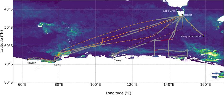
R. S. Humphries et al.: Southern Ocean latitudinal gradients of cloud condensation nuclei                                12761

Figure 1. The voyages tracks from MARCUS (various orange tracks) and CAPRICORN2 (red track) overlaid on MODIS Aqua chl a
concentrations averaged over the measurement period from November 2017 to March 2018. Grey markers show voyage locations where
exhaust-free data were obtained.

cause of the size selection and the refractory nature of sea     water. The sample was then preserved using 1 % chloro-
salt, the actual concentrations reported for chlorine have yet   form. Anion and cation concentrations are determined with
to be calibrated to obtain a correction factor, and values are   a Dionex ICS-3000 reagent-free ion chromatograph. An-
only used in a relative manner in this paper. Ammonium ni-       ions are separated using a Dionex AS17c analytical column
trate and sulfate calibrations were run prior to and after the   (2×250 mm), an ASRS-300 suppressor and a gradient eluent
voyage, as is standard operating procedure.                      of 0.75 to 35 mM potassium hydroxide. Cations are separated
   During CAPRICORN2, time-integrated aerosol composi-           using a Dionex CS12a column (2 × 250 mm), a CSRS-300
tion measurements were made alongside the online ACSM            suppressor and an isocratic eluent of 20 mM methanesulfonic
measurements using a PM1 size-selective inlet (BGI SCC           acid. All values reported in this paper are blank-corrected.
model 2.229, Butler, NJ, USA) and 47 mm quartz filters.             Aerosol composition data measured by the ToF-ACSM
Each filter sampled for 1–2 d (20–48 h) at a flow rate of        and on the PM1 filters during CAPRICORN2 are available
16.67 vLPM (required for the size-selective inlet) controlled    at Humphries et al. (2021a).
by a MFC (Alicat Scientific Model MC 20SLPM). To pre-
vent the filters being contaminated (and overwhelmed) by         2.3   Platform exhaust
exhaust aerosol, the system was placed on a switching con-
troller, which ceased sampling when relative winds direc-        Removal of exhaust contaminated data is a critical step
tions were between 90 and 270◦ and CN concentrations were        required before using any aerosol composition data from
above a threshold value. This meant the PM1 sampling sys-        diesel-powered ship platforms. For aerosol data, exhaust sig-
tem was switched on and off throughout the sampling pe-          nals are typically orders of magnitude higher than ambient
riod so that total volumes through each filter ranged between    data, given the strength and proximity of the source to mea-
14 and 26 m3 . The instantaneous volumetric flow rate from       surement points. Other sources of contaminated air, for ex-
the MFC was recorded and totalled by a electronic flow to-       ample, the incinerator and indoor air vents, are minor in com-
taliser (Amalgamated Instruments Co., model PM4-IVT-DC-          parison with the exhaust but are captured through the filter-
8E, Hornsby, NSW, Australia).                                    ing process described below, largely because these vents are
   Five field blanks were collected approximately weekly         co-located with engine exhaust emissions and have a simi-
throughout the campaign. Field blanks involved carrying out      lar effect on measurements, albeit smaller. The engine age,
the full filter change process with the sample pumps remain-     fuel type, ship architecture (e.g. how the air flows around the
ing switched off. After sampling, filters were enclosed in       ship and creates local eddies), relative locations of exhaust
clean aluminium foil and frozen until they could be anal-        and air sampling inlet, as well as the operations of the ship
ysed post-voyage. The soluble ion concentrations were deter-     during measurements, also affect how much impact the ex-
mined using high-performance anion-exchange chromatog-           haust has on the atmospheric measurements. MARCUS was
raphy with pulsed amperometric detection (HPAEC-PAD)             undertaken aboard the Aurora Australis, an ice-breaker com-
measured at the CSIRO laboratories in Aspendale, Victoria.       missioned in 1989, powered by two Wärtsilä medium-speed
The filters were extracted in 10 mL of 18.2 m deionised         diesel engines (one 16V32D and one 12V32D, producing a

https://doi.org/10.5194/acp-21-12757-2021                                      Atmos. Chem. Phys., 21, 12757–12782, 2021

12762                           R. S. Humphries et al.: Southern Ocean latitudinal gradients of cloud condensation nuclei

total of 10 000 kW) and burning standard marine grade fuel         proximately 500 hourly data points for CCN over the 129 d
oil. As shown in Fig. A1, the ARM measurement container            at sea. In contrast, over 86 % of data during CAPRICORN2
was located directly adjacent to the exhaust pipe of the ship,     was exhaust-free, resulting in over 760 hourly data points
meaning that a large proportion of wind conditions were able       from the 42 d campaign. An example time series of MAR-
to push exhaust into the sampling inlet. The MARCUS cam-           CUS CCN data and the amount of data removed by exhaust
paign was also supplementary to the usual resupply voyages         filtering is shown in Fig. A2. Overlaid on Fig. 1 ship tracks
of the Australian Antarctic Program, and consequently, the         are the locations where exhaust-free data exist for the cam-
direction of the ship was rarely optimal for atmospheric mea-      paigns. Despite the significant data loss associated with ex-
surements – instead being more focused on swell and sea-ice        haust contamination, the latitudinal coverage of the data is
conditions.                                                        reasonable, with each of the 5◦ latitudinal bins having over
   In comparison, the CAPRICORN2 voyage was undertaken             110 data points in each, with the bins south of 60◦ S contain-
aboard the RV Investigator, which was purpose-built for ma-        ing over 450 data points (as shown in Fig. 2).
rine science and specifically incorporated atmospheric mea-
surements into its design, resulting in an architecture opti-      2.4   Trajectory analyses
mised for minimal exhaust impact. The atmospheric sam-
pling inlet is located as far forward on the vessel as pos-        The HYSPLIT (HYbrid Single-Particle Lagrangian Inte-
sible (see Fig. A1), resulting in a significant distance from      grated Trajectory) model (Draxler and Hess, 1998) was used
the exhaust. The ship itself is powered by three nine-cylinder     to calculate air parcel trajectories. In this study, HYSPLIT
MaK diesel engines coupled to a 690 V AC generator and             was used to calculate back trajectories in order to evaluate
burns automotive-grade diesel fuel (as opposed to residual         source regional and vertical source locations for the vari-
(heavy) fuel oil used by most vessels). During the CAPRI-          ous categories. Trajectories were calculated using the Global
CORN2 voyage, the ship was largely positioned to face di-          Data Assimilation System (GDAS) reanalysis (Kanamitsu,
rectly into the wind, ideal for marine conductivity, temper-       1989). The model was set up to utilise 1◦ horizontal res-
ature and depth (CTD) measurements occurring during the            olution reanalysis data, and the vertical motion was calcu-
voyage, and, where possible, transits between marine targets       lated using the model vertical velocity method. Calculations
were optimised for favourable wind conditions to maximise          utilised surface-invariant geopotential, surface 10 m horizon-
the collection of exhaust-free atmospheric data.                   tal (U and V ) winds, 2 m surface temperature and U , V , W
   On both platforms, wind direction was found to be a             (vertical wind), temperature and humidity on pressure lev-
poor parameter for filtering exhaust (Humphries et al., 2019),     els from 1000 to 20 hPa. Each trajectory calculation provided
likely because of the eddies that form around the ship’s su-       hourly three-dimensional air parcel locations for a total time
perstructure and create differences between wind directions        span of up to 5 d in order to limit uncertainty magnification.
measured by meteorological instruments and those experi-           Trajectories were initiated at the ship’s location for every
enced at measurement height. Instead, we used differences in       hour of the cruise at heights of 10 m and represent heights
composition between the exhaust and clean background air           above ground level.
to identify and remove exhaust influence. The exhaust was             Once calculated, trajectories were divided into 5◦ latitu-
identified the same way on both platforms. A first pass was        dinal bins based on their starting location. Only trajectories
undertaken using the automated exhaust identification algo-        corresponding to exhaust-free aerosol data were used. For
rithm described in Humphries et al. (2019). This algorithm         each set of latitudinally binned trajectories, frequency plots
was designed to strike a balance between accurately remov-         were calculated by summing the number of times trajectories
ing obvious exhaust signals but not being too overzealous          passed through a map, binned such that the horizontal reso-
and unwittingly removing clean data. This balance results in       lution of the boxes was 0.5◦ and with linearly spaced, 10 m
the correct removal of about 95 % of exhaust signals. Man-         vertical bins. Resulting plots were smoothed using the ker-
ual filtering is undertaken as the next step and identifies any    nel density estimations using Gaussian kernels (implemented
rapid increases in CN, black carbon, carbon monoxide or car-       with Python SciPy’s guassian_kde function). The bandwidth
bon dioxide concentrations and, in the case of the Aurora          was determined by taking the average effective samples in
Australis, any drops in ozone resulting from titration from        each bin calculated using Scott’s factor (Scott, 2015).
engine-produced nitrogen oxides. It is noted here that the CN         Total precipitation along each trajectory was calculated us-
data are relied on most heavily during this process because        ing ERA-5 reanalysis data (ECMWF, 2018, variable name
of their high time resolution and highest sensitivity to the ex-   “tp”, hourly time steps with spatial grids of 0.25◦ in both lat-
haust signal, which typically changes by orders of magnitude       itude and longitude). For each step in each trajectory, the pre-
relative to background data.                                       cipitation at the time and location was retrieved from the re-
   Because of the differences between the platforms and ship       analysis data, and then the values for each step were summed,
operations, the resulting proportion of clean data available       resulting in a single total precipitation value for each trajec-
for each campaign was significantly different. For MAR-            tory. As before, only trajectories corresponding to exhaust-
CUS, only 11 % of data was exhaust-free, resulting in ap-          free measurement periods were included in the analysis.

Atmos. Chem. Phys., 21, 12757–12782, 2021                                          https://doi.org/10.5194/acp-21-12757-2021

R. S. Humphries et al.: Southern Ocean latitudinal gradients of cloud condensation nuclei                                      12763

3   Results                                                          ern Ocean mid-latitudes. Cape Grim values are markedly
                                                                     higher for CN10 and non-baseline selected CCN data and
Despite the significant removal of data due to exhaust in the        generally agree well with ship data in the respective latitu-
MARCUS campaign, the utilisation of the CAPRICORN2                   dinal bin. Cape Grim baseline data appear to be lower than
campaign data, which occurred at the same time in the same           ship-based measurements in their respective latitudinal bin,
regional area, meant that division of the data into 5◦ latitu-       which may be explained by ship data not being filtered for
dinal bins resulted in sample numbers high enough to cal-            baseline criteria and are consequently likely to include some
culate robust statistics in each bin, while having reasonable        level of continental/anthropogenic influence. Non-baseline
latitudinal resolution. In Fig. 2, violin plots show measure-        CN10 data from Cape Grim are higher than those measured
ments’ distribution in each latitudinal bin for each of CCN0.2 ,     on the ship, and this is likely because of the influence of fine-
CCN0.5 and CN10 (full statistics for each bin are presented          mode aerosol emissions from the metropolitan region of Mel-
in Table A1, and latitudinal gradients for each voyage for           bourne, as well as emissions from Tasmania, both of which
CCN0.5 and CN10 are presented in Figs. A3 and A5, respec-            can influence Cape Grim measurements in non-baseline con-
tively). The highest concentrations (means of 169, 322 and           ditions. Curiously, ship-based CCN data are similar to non-
681 cm−3 for CCN0.2 , CCN0.5 and CN10 , respectively) for            baseline Cape Grim data and significantly higher than base-
all parameters are unsurprisingly observed in the northern-          line data (which is actually similar to the higher latitude
most bin, 40–45◦ S, which is closest to the coast of Tasma-          bins), which suggests ship-based measurements were influ-
nia, Australia, resulting in increased continental and anthro-       enced significantly by continental sources while measuring
pogenic influence. Moving south, CN10 concentrations ap-             at these latitudes, a result confirmed by trajectory analyses
pear to be stable (300–400 cm−3 ) from 45◦ S to 65◦ S. This is       presented later in the paper.
not the case with CCN at both supersaturations, which show              Most striking in the latitudinal distribution is the sta-
slightly elevated concentrations in the 45–50◦ S bin (131 and        tistically significant increase in all aerosol parameters in
197 cm−3 for CCN0.2 and CCN0.5 , respectively), after which          the southernmost bin along the Antarctic coastline (p <
it becomes reasonably constant from 50 to 65◦ S (∼ 100 and           0.001 compared to 60–65◦ S bin). While most pronounced
150 cm−3 , respectively).                                            in CCN0.5 (mean concentrations increase by 50 % com-
   Measurements taken from nearby land-based research sta-           pared to mid-latitudes with 30 % increases for both CCN0.2
tions at Macquarie Island (54◦ 300 S, 158◦ 570 E; Humphries,         and CN10 ), corresponding changes are also apparent in the
2020) and Cape Grim (40◦ 390 S, 144◦ 440 E; Gras and Key-            CCN/CN ratio, wind speed and more significantly in pre-
wood, 2017) were utilised for comparison with the ship-              cipitation, as shown in Fig. A7. It is likely that the larger
based measurements considered here. Macquarie Island is              increase in CCN0.5 relative to CCN0.2 in this bin is a re-
one of the research stations visited as part of the seasonal re-     sult of the changing size distributions and aerosol composi-
supply operations undertaken by the Aurora Australis during          tion when moving between air masses. To explore this ap-
MARCUS (voyage 4 of the 2017/18 ship schedule), and con-             parent change in composition further, we examined more
sequently, data from MARCUS and from the land station are            closely the CAPRICORN2 data which provided both real-
directly comparable. In addition, the upwind fetch of Mac-           time and filter-based aerosol composition data. Latitudinal
quarie Island is dominated solely by the Southern Ocean, so          aerosol composition data from this voyage are shown in
other voyage data at these latitudes, which happen to all be         Fig. 3 alongside binned wind speed and precipitation data.
within the upwind fetch of Macquarie Island, are also com-              While the increase in this southernmost bin was not sig-
parable. The Cape Grim station is classified as a global sta-        nificant in the MARCUS CCN0.2 data, CAPRICORN2 data
tion in the Global Atmospheric Watch station, being repre-           (Figs. 3, A3, A4, A5, A6) show significant increases in
sentative of a globally significant region, so although the lo-      CCN at all supersaturations, in the CCN/CN ratios, as
cation is a reasonable distance from the ship measurements,          well as changes in the dominant species contributing to the
we use the data here with confidence. In Fig. 2, the median          aerosol composition (Fig. 3). Andreae (2009) found that the
values from November 2017 to March 2018 (chosen to co-               CCN0.4 /CN ratios from a wide range of environments av-
incide with the MARCUS campaign period) are presented                eraged 0.4, agreeing well with mid-latitude data from this
from both stations for each available parameter and overlaid         study but highlighting the unique nature of the polar popu-
on the latitudinal gradients in their respective latitudinal bins.   lations. Aerosol composition further south is dominated by
Two datasets are presented for Cape Grim: all data (red) and         sulfur-based particles, consistent with the established litera-
baseline data (green). Baseline refers to periods that repre-        ture (e.g. Fossum et al., 2018; Schmale et al., 2019), whose
sent a clean marine background with fetches from the South-          relative contribution to aerosol mass (as measured by the
ern Ocean with little to no continental influence (Gras and          ToF-ACSM) was around 60 %–70 % at lower latitudes but
Keywood, 2017).                                                      increased to its maximum in the southernmost bin, reaching
   For both CCN and CN data, values measured at Mac-                 over 80 %. We note here that while trends from the filters
quarie Island agree well with those measured aboard the              are similar to those observed on from the ToF-ACSM, the
ships and are likely to be a good representation of South-           differences observed are likely the result of different sam-

https://doi.org/10.5194/acp-21-12757-2021                                          Atmos. Chem. Phys., 21, 12757–12782, 2021
12764                             R. S. Humphries et al.: Southern Ocean latitudinal gradients of cloud condensation nuclei

Figure 2. Latitudinal distributions of CCN (at (a) 0.2 % and (b) 0.5 % supersaturation) and CN10 (c) from collated data from both MARCUS
and CAPRICORN2 campaigns shown in blue. Data are binned into 5◦ latitudinal bins and plotted as violin plots with medians (circles) and
25th and 75th percentiles (grey box) shown. Data from November 2017 to March 2018 from Macquarie Island (54◦ 300 S, 158◦ 570 E; orange)
and Cape Grim (40◦ 390 S, 144◦ 440 E; left, green is baseline (Rn < 100 mBq, wind directions between 190 and 280◦ ); red is all data) at their
respective latitudinal bins. Subplots above each plot show the number of hourly data points in each bin. Note the y-axis scales are custom for
each dataset.

pling techniques: the ToF-ACSM measures non-refractory                   hour of exhaust-free data during the five voyages. In Fig. 4,
aerosol composition, while the filters are analysed for sol-             these trajectories, split into the six latitudinal bins based on
uble ions. The increases in CCN ratio could be driven by                 each trajectory’s end location, are shown as density plots.
a stronger source of sulfur precursors (sulfate and MSA de-              As expected, the northernmost bin shows influence primarily
rived from DMS) emitted from enhanced phytoplankton near                 from the marine boundary layer upwind of the measurements
the Antarctic continent (Fig. 1) but are likely to also be driven        and significant influence from both Tasmania and the more
by a significant drop in precipitation which would preferen-             heavily populated areas of south-eastern Australia. This tra-
tially scavenge CCN compared to other aerosols. Chloride,                jectory footprint is consistent with CN10 ship values in this
which is used as a proxy for sea spray aerosol, is observed to           bin being higher than baseline values at Cape Grim (Fig. 2),
be dominant at lower latitudes (and varies proportionately to            where these continental and anthropogenic influences are ex-
wind speed; Fig. A9) but reaches its minimum in the high-                cluded. Note that non-baseline values from Cape Grim are
latitude bin. This significant reduction in the high-latitude            higher than those from the ship-measurements in this bin,
bin is consistent with the combined effect of decreased wind             despite similar source regions. This is likely to be explained
speeds and the occurrence of sea ice covering the ocean sur-             simply by the closer proximity of Cape Grim to these anthro-
face, resulting in a substantially lower source strength, which          pogenic sources than the ship measurements. For bins from
outweighs the reduced precipitation sink. Interestingly, com-            45 to 60◦ S, all fetches reside within the Southern Ocean’s
parison of the distributions of CCN with the sulfur and chlo-            marine boundary layer upwind of the measurements, with
ride composition measurements suggests that while sea-salt               only a small subset of trajectories arriving from the free tro-
aerosol contributes an important baseline to CCN numbers,                posphere. Unlike other bins, the southernmost bin has fetches
the variability, and in particular the vast population of CCN            that consist primarily of coastal and Antarctic continental
at high latitudes, is driven by sulfur-based aerosols, similar           latitudes, with minimal marine influence. The altitude plot
to what has been reported by Vallina et al. (2006) and oth-              shows the boundary layer influence is significantly reduced,
ers. Recent work by Fossum et al. (2020) suggests an inverse             and instead, fetches are distributed across a range of heights
relationship between sea-salt aerosol concentrations and sul-            in the troposphere. Interestingly, the 60 to 65◦ S bin is a mix
fate CCN activation, which could also help to explain this               of marine boundary layer and free tropospheric fetches and
change in the southernmost bin.                                          is likely a result of the atmospheric polar front varying at lat-
   To further understand the source regions of the observed              itudes covered by this bin.
latitudinal changes, we calculated the trajectories for each

Atmos. Chem. Phys., 21, 12757–12782, 2021                                                  https://doi.org/10.5194/acp-21-12757-2021

R. S. Humphries et al.: Southern Ocean latitudinal gradients of cloud condensation nuclei                                           12765

Figure 3. Latitudinal distributions for parameters measured during CAPRICORN2 highlighting the aerosol composition and source and sink
mechanisms. The CCN/CN10 ratios for 0.2 % and 0.5 % supersaturation are shown in (a) and (b), respectively; the major aerosol chemical
components from the ToF-ACSM in (c); and the total soluble ions from PM1 filters in (d). Panel (e) shows the wind speed measured onboard
the vessel, and (f) shows the total precipitation calculated using ERA5 reanalysis data along the backward trajectory for each measurement.
Note that in (c), the sulfate is split to the left axis to enable better visibility of trends of other components.

   The trajectory analysis shows the air-mass histories in the          ences of air-mass transport, the properties of the aerosol pop-
region are consistent with more detailed trajectory studies             ulations differ. For example, if high-latitude transport path-
undertaken previously (Humphries et al., 2016; Alroe et al.,            ways take the bulk of phytoplankton emissions from the sea-
2020). In particular, measurements from the mid-latitudes               ice region into the Antarctic free troposphere before being
of the Southern Ocean are found to have air mass histories              brought back to the surface (as proposed by Humphries et al.,
confined primarily to the marine boundary layer, whereas                2016), the increased precursor concentrations may result in
the closer the approach to the East Antarctic continent, the            more aerosol nucleation and growth in the free troposphere,
greater the influence from the free troposphere of the po-              resulting in the enhanced CCN concentrations observed in
lar cell. These large-scale air-flow differences are likely the         the high-latitude bin. In addition, free tropospheric aerosols
leading cause of the differences between the mid- and high-             would be less exposed to the high surface area of sea-salt
latitude aerosol properties measured in this study. Given the           aerosols that typically dominate the aerosol mass in the ma-
remoteness of the region and the limited number of aerosols             rine boundary layer and so would be less likely to be scav-
sources, typically phytoplankton emissions and sea spray, it            enged, resulting in the higher CCN number concentrations.
is likely that the aerosol sources are consistent across all
latitudes. However, differences observed in the atmosphere
are driven by two factors: (1) air-mass fetches alter the ef-
ficiency and strength of the sea-salt source and (2) sources
of secondary aerosols are the same, but because of the differ-

https://doi.org/10.5194/acp-21-12757-2021                                              Atmos. Chem. Phys., 21, 12757–12782, 2021

12766 R. S. Humphries et al.: Southern Ocean latitudinal gradients of cloud condensation nuclei
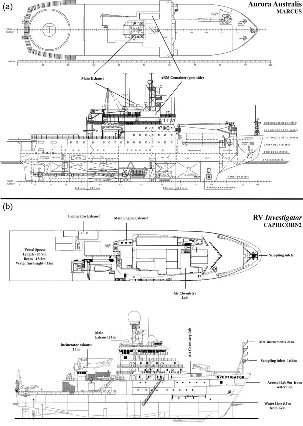
Figure 4. Trajectory frequency plots showing the spatial footprint of measurements in each latitudinal bin in each dimension. Five-day
backward trajectories were calculated for each hour of valid, exhaust-free data, and then the number of times trajectories passed through 0.5◦
bins was summed before smoothing, resulting in frequency plots. Map plots are shown in the left column, with the starting locations of each
of the trajectories used for each binned plot shown in black. The right column shows the frequency plots as a function of time and altitude,
giving an indication of the dominant atmospheric layers important in each region.
4 Discussion mid-latitude sector (45–65◦ S); and the high-latitude coastal
region of Antarctica (65–70◦ S).
Unsurprisingly, the northern sector exhibits the most an-
thropogenic and continental influence, resulting in aerosol
These data suggest that there are three distinct latitudinal re- concentrations approximately twice that of those in the open
gions that govern the Southern Ocean aerosol populations in Southern Ocean for both CN10 and CCN0.5 . For CCN0.2 , this
the summer season: the northern sector north of 45◦ S; the
Atmos. Chem. Phys., 21, 12757–12782, 2021 https://doi.org/10.5194/acp-21-12757-2021R. S. Humphries et al.: Southern Ocean latitudinal gradients of cloud condensation nuclei 12767 distinction is not so clear, suggesting that the same source CCN concentration at 0.02 % supersaturation during leg 2 as mid-latitudes is driving CCN concentrations at this su- was 111 cm−3 , similar to the concentrations measured south persaturation (presumably sea salt). This would suggest that of 65◦ S in this study, and the fraction of CN acting as CCN aerosols arising from anthropogenic and continental sources was highest near the Antarctic continent, also observed in our are less hygroscopic than sea salt, which is consistent with study. Schmale et al. (2019) suggested this could be due to what is expected from the literature (e.g. Swietlicki et al., differences in aerosol chemical composition, with a combi- 2008). nation of many cloud processing cycles and greater supply of The mid-latitude observations are consistent throughout DMS oxidation products resulting in particles large enough a large range of latitudes, being dominated by sea-salt and to act as CCN. sulfur-based aerosols (Fig. A9). Given the lack of any land Contrary to the West Antarctic region, the region of the masses in this region, the primary aerosol sources are driven East Antarctic coast included in this study is not well rep- by wind-produced sea salt and secondary aerosol forma- resented by measurements on the Antarctic continent it- tion, typically resulting from both local and long-range trans- self, a phenomenon driven by well defined air-mass trans- port of aerosol precursors emitted from biological sources, port, which isolates the continent from the sea-ice region chiefly DMS from phytoplankton. The dependence of sea- (Humphries et al., 2016). This result was true for springtime salt aerosol concentrations on wind speed and precipitation measurements, and further work by the same authors (cur- is striking, being directly and inversely proportional, respec- rently unpublished) suggests that the meteorology that leads tively. This relationship breaks down in the high-latitude to this phenomenon may break down both during summer- bins, where sea-ice cover impacts the wind mechanism of time and around the Antarctic Peninsula. Since the majority sea-salt aerosol production. of measurements in the region occur in summer and at ei- While observations in both the northern and mid-latitudes ther Antarctic stations or at lower latitudes, the East Antarc- have been noted previously in the literature, the high-latitude tic coastal region remains one of the more poorly represented observations are novel. This is in part driven by how remote regions of the world. the region is and how infrequently it has been sampled in The change in aerosol properties at this high-latitude bin is the past (e.g. high-latitude Southern Ocean measurements consistent with the crossing of the Antarctic atmospheric po- off East Antarctica are reported only by Humphries et al., lar front, as first described by Humphries et al. (2016) and ob- 2016; Alroe et al., 2020; Simmons et al., 2021; Schmale served by both Alroe et al. (2020) and Simmons et al. (2021). et al., 2019). For example, the recent SOCRATES aircraft While values observed in this paper are in line with those pre- campaign (McFarquhar et al., 2021) involved measurements viously observed across the polar front (Alroe et al., 2020; made on flights originating from Hobart. However, because Simmons et al., 2021), this dataset adds confidence that the of the limited range of the aircraft, measurements could only change observed in these previous studies is an enduring phe- be made to 62◦ S, so that the significant change in aerosol nomenon across a wider range of East Antarctic longitudes populations at higher latitudes could not be observed. and seasons. While the definition of the Antarctic polar cell Measurements have been made in other parts of the is traditionally understood in terms of climatological aver- Antarctic sea ice (e.g. Davison et al., 1996; Fossum et al., ages, it is evident that a very real-time boundary exists that 2018; Schmale et al., 2019). Typically, these sectors do not can be seen in the atmospheric composition observations, show the step changes observed in the East Antarctic sea-ice which is not necessarily observed in the meteorological vari- measurements and instead are reasonably well represented ables from which it is typically defined (i.e. a sharp change by continental measurements (e.g. Asmi et al., 2010; Hansen in wind direction and air temperature). Because of this, and et al., 2009; Hara et al., 2011; Ito, 1993; Järvinen et al., 2013; to create a distinction from the traditionally defined meteo- Koponen et al., 2003; Pant et al., 2011; Samson et al., 1990; rological front, we introduce a new term to define it here as Virkkula et al., 2009; Weller et al., 2011; Hara et al., 2020). the Atmospheric Compositional Front of Antarctica (ACFA), During a campaign around the Antarctic Peninsula in sum- which represents the northern boundary of the region that mer 2015, Fossum et al. (2018) observed two distinct air extends south to approximately the Antarctic coastline – a masses: those coming from continental Antarctica and those region we term the Antarctic Sea Ice Atmospheric Composi- from the marine region north of the polar front. They found tional Zone (ASIACZ). It is important to note that while the that, despite the differing composition of the two air masses aerosol properties in the ASIACZ are not captured by sur- which reflected observations described in this paper (i.e. a face measurements on the Antarctic continent, nor those in decrease in sea salt in air masses from the south), CCN con- the Southern Ocean mid-latitudes, trajectory studies suggest centrations at realistic supersaturations for this region (0.3 %) that air masses from this region travel both north and south, remained relatively constant at around 200 cm−3 . Schmale typically above the boundary layer (Humphries et al., 2016), et al. (2019) report CCN concentrations determined while making this an important region of exporting aerosols and circumnavigating Antarctica between December 2016 and precursors from a highly biologically productive region to March 2017, with leg 2 of the voyage passing closest to other regions. This could help reconcile the predicted miss- the Antarctic continent (mainly West Antarctica). Median ing aerosol source in the wider region. https://doi.org/10.5194/acp-21-12757-2021 Atmos. Chem. Phys., 21, 12757–12782, 2021
12768                          R. S. Humphries et al.: Southern Ocean latitudinal gradients of cloud condensation nuclei

   The ACFA is known to vary in time and space and can be        possible that different patterns may be observed in other sec-
advected by the synoptic-scale meteorology. This is evident      tors of the Southern Ocean that are influenced by disparate
from the individual voyage latitudinal plots (Figs. A3 and       continental influences, such as those around Africa and South
A5), where the increases in the southernmost bin latitudes       America. Hence, it is important that future observation cam-
differ depending on the voyage and location. This movement       paigns investigate these regions. While important circum-
can even occur within a single voyage, as evidenced clearly      polar measurements such as those undertaken by Schmale
from the CAPRICORN2 voyage data (Figs. A3 and A8),               et al. (2019) give an insight into this variability, campaign
where the increase in CCN occurred at approximately 64◦ S        measurements are limited in their duration and are generally
during one crossing at 150◦ E and 62.5◦ S during the 140◦ E      undertaken during the summertime (e.g. Humphries et al.,
transect. During this voyage, we also tried to intentionally     2016; Fossum et al., 2018). To avoid biases that may arise
cross the front while sampling south along the 132◦ E merid-     by applying these conclusions to other seasons, long-term
ian. However we were unable to locate the front, even when       measurements, such as those undertaken at Cape Grim and
travelling further south (> 65◦ S) of the ACFA’s latitude just   at Cape Point, South Africa (Labuschagne et al., 2018), and
days before.                                                     by the RV Investigator are needed across other longitudes of
   By investigating latitudinal gradients across the parts of    the Southern Ocean. These include remote sites such as Mac-
the Southern Ocean, this work raises some important objec-       quarie Island (measurements included here were limited to
tives for future work. A significant motivation for this work    just 2 years) and research platforms that frequent the ASI-
is to better inform and reconcile the radiation biases aris-     ACZ, such as the soon-to-be commissioned RSV Nuyina.
ing from poor representation of clouds in climate and earth      Long-term year-round atmospheric aerosol datasets reveal
system models. Hence, relating these observations to recent      important seasonal and annual variability and the processes
cloud observations is important, and this work is well un-       that contribute to this variability. Hence, these data will be
derway. Mace et al. (2021) analysed MARCUS and CAPRI-            critical for ensuring reduced biases in modelling efforts.
CORN2 data and found gradients in cloud droplet number
concentrations in reasonable agreement with the gradients in
CCN concentrations identified here. Interestingly, Mace et al.   5   Conclusions
(2021) observed a bimodal distribution in cloud properties
poleward of 62.5◦ S. While one mode displayed properties         In this paper we collated data from two intensive research
of marine clouds from farther north, the second showed rel-      campaigns, spanning five voyages in the Southern Ocean re-
atively high cloud droplet numbers and low effective radii.      gion between Australia and East Antarctica. Aerosol micro-
The bimodality was inferred to be associated with changes        physical and chemical properties were assessed in terms of
in air mass properties (such as CN, CCN and aerosol chem-        the latitudinal variability. Three main latitudinal regions were
istry), identified in previous work (Humphries et al., 2016),    identified: the northern sector north of around 45◦ S, where
in case study events described in Mace et al. (2021) and in      continental and anthropogenic sources add to the background
further analysis of CAPRICORN 2 data currently underway.         marine atmosphere; the mid-latitudes (45–65◦ S), where the
In particular, these changes in air mass properties included     marine boundary layer populations dominate; and the far
those identified systematically in this work (i.e. high CCN      south (65–70◦ S), termed here as the Antarctic Sea Ice Atmo-
and CCN/CN and high sulfate and MSA indicative of bio-           spheric Compositional Zone (ASIACZ), where aerosol pop-
genic aerosol sources) in the southern sector. The potential     ulations are dominated by sulfur-based species derived from
sensitivity of the cloud properties to these biogenic aerosol    free-troposphere nucleation, and sea spray aerosol is signif-
sources suggests a strong feedback with biological and pho-      icantly reduced. Aerosol concentrations were highest in the
tochemical activity in the region, an issue that warrants fur-   northern and southern bins, with CCN0.5 concentrations be-
ther and extensive investigation.                                ing approximately 70 % higher than mid-latitude concentra-
   Further studies should also address the transition across     tions of around 150 cm−3 . Simultaneous measurements from
the ACFA. A more detailed assessment of the datasets used        nearby land-based stations were compared with these ship-
in this paper that focuses on the transition and the chemi-      board measurements and were found to be good representa-
cal and physical changes that occur in gases, aerosols and       tions of their respective latitudes, with the long-term baseline
clouds in this region is currently underway and will be de-      measurements at Cape Grim being representative of CCN
scribed in a future publication. The comprehensive, continu-     at all northern and mid-latitudes and CN10 at the northern
ous measurements aboard the RV Investigator also provide a       sector. Measurements from a 2-year campaign at the sub-
perfect opportunity for understanding transition as the vessel   Antarctic station of Macquarie Island (54◦ 300 S, 158◦ 570 E)
frequently undertakes voyages into this region – albeit pri-     were found to be representative of the mid-latitudes for all
marily limited to the summertime.                                species. The ASIACZ region was not represented by either
   These conclusions are all based on the sector of the South-   of these stations, and previous work suggests that measure-
ern Ocean between Australia and the East Antarctic and are       ments at research stations on the Antarctic continent are not
only valid for late spring and summer measurements. It is        reflective of this spatially significant region. Further mea-

Atmos. Chem. Phys., 21, 12757–12782, 2021                                        https://doi.org/10.5194/acp-21-12757-2021
You can also read