Something fishy going on? Evaluating the Poisson hypothesis for rainfall estimation using intervalometers: results from an experiment in Tanzania ...
←
→
Page content transcription
If your browser does not render page correctly, please read the page content below
Atmos. Meas. Tech., 14, 5607–5623, 2021
https://doi.org/10.5194/amt-14-5607-2021
© Author(s) 2021. This work is distributed under
the Creative Commons Attribution 4.0 License.

Something fishy going on? Evaluating the Poisson hypothesis for
rainfall estimation using intervalometers: results from an
experiment in Tanzania
Didier de Villiers1 , Marc Schleiss2 , Marie-Claire ten Veldhuis1 , Rolf Hut1 , and Nick van de Giesen1
1 Department  of Water Management, Faculty of Civil Engineering, Delft University of Technology, Delft, the Netherlands
2 Department  of Geoscience & Remote Sensing, Faculty of Civil Engineering, Delft University of Technology,
Delft, the Netherlands

Correspondence: Didier de Villiers (d.j.devilliers@tudelft.nl)

Received: 3 May 2020 – Discussion started: 22 June 2020
Revised: 15 June 2021 – Accepted: 6 July 2021 – Published: 17 August 2021

Abstract. A new type of rainfall sensor (the intervalome-         tipping bucket measurements. Intervalometer estimates of to-
ter), which counts the arrival of raindrops at a piezo elec-      tal rainfall amount overestimate the co-located tipping bucket
tric element, is implemented during the Tanzanian monsoon         measurement by 12 %. The intervalometer principle shows
season alongside tipping bucket rain gauges and an impact         potential for use as a rainfall measurement instrument.
disdrometer. The aim is to test the validity of the Poisson
hypothesis underlying the estimation of rainfall rates using
an experimentally determined raindrop size distribution pa-
rameterisation based on Marshall and Palmer (1948)’s ex-          1   Introduction
ponential one. These parameterisations are defined indepen-
dently of the scale of observation and therefore implicitly as-   Africa, and particularly Sub-Saharan Africa, is one of the
sume that rainfall is a homogeneous Poisson process. The          most vulnerable regions in the world to climate change (Boko
results show that 28.3 % of the total intervalometer observed     et al., 2007). The main economic activity (by share of labour)
rainfall patches can reasonably be considered Poisson dis-        is agriculture, with 98 % of crop production being rainfed
tributed and that the main reasons for Poisson deviations         (Abdrabo et al., 2014). At the same time, much of Sub-
of the remaining 71.7 % are non-compliance with the sta-          Saharan Africa is greatly underserviced by weather obser-
tionarity criterion (45.9 %), the presence of correlations be-    vations, and the existing observational networks have been
tween drop counts (7.0 %), particularly at higher arrival rates   in decline since the mid-1990s; from an average of eight
(ρa > 500 m−2 s−1 ), and failing a χ 2 goodness-of-fit test for   stations per 1 million square kilometres, the density has de-
a Poisson distribution (17.7 %). Our results show that whilst     creased to less than one in 2015 (data from the Climate Re-
the Poisson hypothesis is likely not strictly true for rainfall   search Unit of the University of East Anglia, 2017). There are
that contributes most to the total rainfall amount, it is quite   some organisations working on setting up new observational
useful in practice and may hold under certain rainfall condi-     networks, such as the Trans-African Hydro-Meteorological
tions. The parameterisation that uses an experimentally de-       Observatory (TAHMO), but progress is slow due to the lack
termined power law relation between N0 and rainfall rate re-      of financial incentives for weather data. As a result, the
sults in the best estimates of rainfall amount compared to        African climate has not been as well researched in compar-
co-located tipping bucket measurements. Despite the non-          ison to those of western Europe and the United States (Otto
compliance with the Poisson hypothesis, estimates of total        et al., 2015; Washington et al., 2006).
rainfall amount over the entire observational period derived         For example, a recent review of weather index insurance
from disdrometer drop counts are within 4 % of co-located         for smallholder farmers (some of the world’s poorest people)
                                                                  found that the sparsity of ground-based weather stations is a

Published by Copernicus Publications on behalf of the European Geosciences Union.
5608                                           D. de Villiers et al.: Evaluating the Poisson hypothesis for rainfall estimation

large challenge for insurers in Sub-Saharan Africa (Greatrex       ity. To borrow Kostinski and Jameson (1997)’s words: “The
et al., 2015), and companies have been forced to look to other     ‘streakiness’ that is part of the lived experience of rainfall can
sources of data or to develop other indices by which to in-        be seen when sheets of rain pass across the pavement during
sure crops. Global rainfall estimates from satellites, such as     thunderstorms.” This clumping results in greater variability
the Global Precipitation Measurement (GPM) mission, are            than is predicted by the Poisson hypothesis.
instrumental in bridging this gap. However, satellite observa-        To overcome these difficulties, two different approaches
tions, whilst providing good spatial coverage, do not cover        have been proposed. Some researchers (e.g. Lovejoy and
the entire temporal period, and the spatial resolution is of-      Schertzer, 1990; Lavergnat and Golé, 1998) proposed to
ten too coarse for local applications. Robust, inexpensive and     abandon the Poisson process framework and replace it with
accurate rainfall measuring instruments would add a lot of         a scale-dependent, multi-fractal representation of rain. Oth-
value by providing ground-based measurements.                      ers proposed to generalise the homogeneous Poisson process
   Satellite retrievals face another issue for areas with a        (with a constant mean) to a doubly stochastic Poisson process
lack of ground-based data for validation. Since both active        or Cox process, where the mean itself is a random variable
(radars) and passive (radiometers or IR sensors) onboard           (Jameson and Kostinski, 1998; Smith, 1993; Cox and Isham,
sensors do not measure rainfall directly, information about        1980).
the microstructure of precipitation is needed in order to de-         The aim of this study is to formally assess the adequacy
velop robust rainfall retrieval algorithms. Information about      of the homogeneous Poisson hypothesis and its importance
the drop size distribution (DSD) in particular is needed to        in deriving rainfall estimates from ground-based measure-
retrieve rainfall rates (R) from radar reflectivity (Z) mea-       ments in a tropical climate. The intervalometer, a new kind
surements observed by, e.g. radars aboard the GPM mission          of inexpensive rainfall sensor, is introduced and tested for
(Munchak and Tokay, 2008; Guyot et al., 2019). A founda-           its suitability in providing ground-based rainfall estimates in
tional work in this regard is the exponential DSD model pro-       Sub-Saharan Africa. To this end, nine intervalometers were
posed by Marshall and Palmer (1948). Since then, a lot of          deployed over a 2-month period during the Tanzanian trop-
work has been done on determining alternative parameteri-          ical monsoon. The Marshall and Palmer (1948) exponential
sations and many different models have been proposed, of           parameterisation as well as two other experimentally deter-
which the most widely used are the exponential, gamma (Ul-         mined exponential parameterisations of the DSD were used
brich, 1983; Tokay and Short, 1996; Iguchi et al., 2017) and       to convert the intervalometer raindrop arrival rates into rain-
lognormal distributions (Feingold and Levin, 1986). It has         fall rates and results were compared with disdrometer and
also been shown that the appropriate parameterisation is de-       tipping bucket measurements. A hierarchical system of sta-
pendent on the type of rainfall (Atlas and Ulbrich, 1977) and      tistical tests on the drop counts was used to assess the validity
the climatic setting (Battan, 1973; Bringi et al., 2003). There-   of the homogeneous Poisson hypothesis. Section 2 presents
fore, ground “truthing” of DSDs for satellite retrievals is very   the experimental setup. The methods of analysis are detailed
important to ensure that the natural variability of the DSD is     in Sect. 3, and the results and discussion are presented in
being correctly taken into account when estimating rainfall        Sects. 4 and 5, respectively. A list of conclusions follows in
rates (Munchak and Tokay, 2008).                                   Sect. 6.
   An assumption that is seldom explicitly mentioned in the
presentation of these parameterisations is the homogeneity
assumption (Uijlenhoet et al., 1999), which states that be-        2     Materials
low some minimum scale, raindrops are distributed homoge-
neously (as uniformly as randomness allows) in space and           2.1    Instruments
time. Otherwise, the parameterisation would depend on the
size of the sample volume, area and/or time period to which it     In total, the experiment made use of nine intervalometers,
pertains. Statistical homogeneity implies that the number of       one acoustic disdrometer and two tipping bucket rain gauges
drops in a fixed volume can be described by a single constant      at eight different sites. The tipping bucket rain gauge was
parameter such as the average drop density per unit volume         made by Onset (more info at https://www.onsetcomp.com/
or the raindrop arrival rate at the surface (Uijlenhoet et al.,    products/data-loggers/rg3, last access: 11 August 2021) in
1999). Such a point process is called a homogeneous or sta-        the US and was equipped with a HOBO data logger; the
tionary Poisson point process, and the number of drops is dis-     acoustic disdrometer was manufactured by Disdrometrics in
tributed according to a Poisson distribution (Uijlenhoet et al.,   Delft, the Netherlands; and the intervalometer was also made
1999). The arrival of raindrops at a surface has long been         by Disdrometrics. The intervalometer is a device that reg-
considered an example of a Poisson process (Kostinski and          isters the arrival of raindrops at the surface of a piezoelec-
Jameson, 1997; Joss and Waldvogel, 1969). However, this as-        tric drum and can be constructed for less than USD 150. It
sumption has been questioned and several studies argue that        has a minimum detectable drop diameter (Dmin ) of 0.8 mm,
the homogeneity assumption is incompatible with the spatial        determined in a lab experiment by Jan Pape. Typical val-
and temporal clumping of raindrops that is observed in real-       ues of Dmin for impact disdrometers are between 0.3 and

Atmos. Meas. Tech., 14, 5607–5623, 2021                                              https://doi.org/10.5194/amt-14-5607-2021
D. de Villiers et al.: Evaluating the Poisson hypothesis for rainfall estimation 5609
0.6 mm (Johnson et al., 2011). The Dmin value of 0.8 mm ping bucket to determine the mean volume and the standard
for the intervalometer means that the instrument is likely deviation (hereafter called SD error) of each tip in the field.
to miss many small drops and underestimate rainfall rates. At higher rainfall rates than 20 mm h−1 , the rainfall accu-
The advantage of the intervalometer over a standard rain mulation amounts may be underestimated (Humphrey et al.,
gauge is that it provides drop counts as well as rainfall 1997).
estimates. More information about the intervalometer can
be found at https://github.com/nvandegiesen/Intervalometer/ 2.3 Data availability
wiki/Intervalometer (last access: 11 August 2021). A simi-
lar instrument in terms of acoustic sensor is also described There were some issues over the course of the experiment
by Hut (2013). The acoustic disdrometer registers the kinetic with the various instruments that affected the availability of
energy of drop impacts at a drum and converts this to an es- data. The disdrometer picked up on a oscillating signal from
timate of the drop size. It is similar to an intervalometer but 20 May 2018 onward that resulted in total corruption of
also provides individual drop size estimates. The minimum the data. Some intervalometers experienced water damage,
detectable drop diameter for the disdrometer was thought to particularly in storms with high rainfall intensities, which
be 0.6 mm but in practice was 1 mm. This is larger than what caused the instruments to go offline for certain periods of
is typical for an impact disdrometer and means that it likely time. Two were damaged beyond repair. The tipping bucket
misses many small drops and underestimates the actual rain- gauges experienced no known issues. Figure 2 presents an
fall rate. The effect of truncation on rainfall estimation is dis- overview of the data available.
cussed in Sect. 3.2. A good discussion of the pros and cons of
impact disdrometers in general can be found in, e.g. (Tokay 3 Methods
et al., 2001; Guyot et al., 2019) and for tipping buckets in,
e.g. Ciach (2003). The tipping bucket rain gauge collects all 3.1 Deriving rainfall rates from rain drop arrival rates
drops over a known surface area and funnels them to a small
bucket which tips whenever a fixed volume of water has been Uijlenhoet and Stricker (1999) present an excellent review of
collected (typically 0.2 mm). The volume of each tip is veri- the exponential DSD parameterisation as well as the deriva-
fied in situ via a field calibration experiment. tions of relevant rainfall quantities. A small summary mostly
derived from their work is presented below. The raindrop size
2.2 Experiment distribution in a volume of air NV (D) [mm−1 m−3 ] is de-
fined such that the quantity NV (D)dD represents the average
In total, eight sites were selected along the southern coast of number of drops with diameters between D and D + dD per
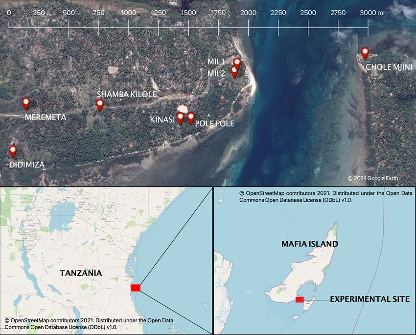
Mafia Island, Tanzania. Figure 1 presents the experimental unit volume of air. Marshall and Palmer (1948) proposed to
layout. Sensors were placed in an approximate line, such that model NV (D) using an exponential model of the form:
a rectangle 3.1 km in length and 500 m in width would cover
all the sites. The dimension of the long axis of the experiment NV (D) = N0 exp(−3D) (1)
was chosen to approximate that of the spatial resolution (ap- 3 = 4.1R −0.21
[mm−1
] (2)
proximately 5 km) of the GPM dual polarisation radar (DPR) 3 −1 −3
instrument. N0 = 8 × 10 [mm m ]. (3)
Rainfall measurement sites were chosen to comply as
If raindrops are assumed to fall at terminal velocity, then
much as possible with World Meteorological Organisation
NV (D) can be related to the DSD of drops arriving at a
guidelines within the constraints of accessibility and land-
unit surface area, NA (D) [mm−1 m−2 s−1 ], by v(D) [m s−1 ],
scape. Ideally, this means that all of the sensors should be
which describes the relationship between drop diameter and
placed in vegetation clearings, sheltered as much as possible
terminal fall velocity. NA (D) is the form of the DSD that
from the wind at a height of 1.5 m off the ground and 1.5 m to
is observed by disdrometers and intervalometers (Uijlenhoet
the nearest instrument (if co-located) and between 2×H and
and Stricker, 1999; Smith, 1993).
4 × H from the nearest object, where H is the difference in
height between the nearest obstacle and the rainfall measure- NA (D) = v(D)NV (D) (4)
ment instrument. All guidelines were followed except for the
H requirement due to dense vegetation within the entire ob- Atlas and Ulbrich (1977) showed that v(D) can be ap-
servational area. In practice, the distance to the nearest object proximated by a power law, v(D) = αD β , with α =
ranged between H and 4 × H . No instruments where placed 3.778 [m s−1 mm−β ] and β = 0.67 [–] providing a close fit
at sites where the nearest obstacle was ≤ H away. Tipping to the data collected on the terminal fall velocity of drops in
buckets were calibrated in the field by dripping 100 mL of stagnant air by Gunn and Kinzer (1949) for 0.5 mm ≤ D ≤
water (from a tripod stand) at a rate slower that 20 mm h−1 5.0 mm. The mean raindrop arrival rate, ρA [m−2 s−1 ], is de-
onto the instrument and recording the number of tips. The fined as the integral over all drop sizes of NA (D). For the
calibration experiment was repeated five times for each tip- intervalometer, this is the integral between Dmin = 0.8 mm
https://doi.org/10.5194/amt-14-5607-2021 Atmos. Meas. Tech., 14, 5607–5623, 2021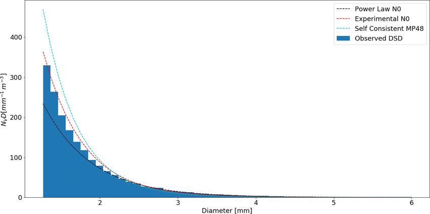
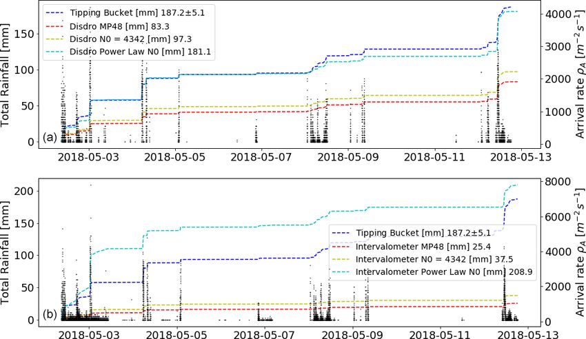
5610                                              D. de Villiers et al.: Evaluating the Poisson hypothesis for rainfall estimation

Figure 1. The eight intervalometer sites on Mafia Island, off the coast of Tanzania. Each site contains one intervalometer. Pole Pole also had
a co-located tipping bucket and impact disdrometer. MIL1 also had a co-located tipping bucket.

Figure 2. Record of the time periods during which the intervalometers collected data for each intervalometer site and the total rainfall amount
[mm] from the tipping bucket at Pole Pole.

Atmos. Meas. Tech., 14, 5607–5623, 2021                                                      https://doi.org/10.5194/amt-14-5607-2021
D. de Villiers et al.: Evaluating the Poisson hypothesis for rainfall estimation                                              5611

and ∞ since the instrument has a minimum detectable drop          rates) or from edge effects (resulting in underestimated rain
diameter of 0.8 mm.                                               rates). Edge effects occur when drops with D > Dmin land
                                                                  near the edges of the sensor, where the signal is damped
         Z∞                      Z∞
                                                                  and may not be recorded properly, especially if D is close
ρA =          NA (D)dD = αN0          D β exp(−3D)dD              to Dmin .
       Dmin                  Dmin                                    There is also model error that arises from the assumption
            0(1 + β, 3Dmin )                                      that the DSD is adequately described by the Marshall and
      = αN0                  ,                             (5)    Palmer (1948) exponential parameterisation rather than some
                 31+β
                                                                  other parameterisation. The parameterisation of the DSD
where 0 is the upper incomplete gamma function (Arfken            with a fixed intercept parameter (N0 = 8000 [mm−1 m−3 ])
et al., 2013). Uijlenhoet and Stricker (1999) presented an        and a slope parameter 3 depending on rain rate according
equation relating the rainfall rate (R) to 3, β, α and N0 , and   to a power law (3 = 4.1R −0.21 [mm−1 ]), such as proposed
noted that for self-consistency purposes the left- and right-     by Marshall and Palmer (1948) derived from stratiform rain-
hand sides of Eq. (6) should be equal:                            fall in Montreal, Canada, may not be applicable in Tanza-
                                                                  nian rainfall, which is of a largely convective nature. Model
                      0(4 + β)
R = 6π × 10−4 αN0              .                           (6)    error will be accounted for by comparing three Marshall
                       34+β                                       and Palmer (1948) type exponential parameterisations of the
This equation can be inverted to give the self-consistent 3–R     DSD. Many parameterisations for the DSD have been pro-
relation. If the DSD is truncated (in this case at Dmin ), then   posed and tested in the literature, of which the most widely
Eq. (6) is modified as follows:                                   used are the exponential (of which the Marshall and Palmer,
                                                                  1948 model is a special case), gamma (Ulbrich, 1983; Tokay
                      0(4 + β, 3Dmin )                            and Short, 1996; Iguchi et al., 2017) and lognormal distribu-
R = 6π × 10−4 αN0                      .                   (7)
                           34+β                                   tions (Feingold and Levin, 1986). These other parameterisa-
                                                                  tions will not be investigated as the focus of this study is to
   For the truncated DSD, the 3–R relation must be solved         test the homogeneity assumption that underlies these models
for numerically. Equation (7) is used in conjunction with the     rather than compare different DSD parameterisations.
α and β values presented by Atlas and Ulbrich (1977) and the         Three separate exponential parameterisation are tested.
Marshall and Palmer (1948) N0 value and a Dmin of 1 mm.           First is the self-consistent Marshall and Palmer (1948) pa-
The rainfall rate is varied from 0.1 to 100 mm h−1 in incre-      rameterisation with the 3–R relation presented in Eq. (8).
ments of 0.1 mm h−1 and for each value of R, 3 is solved for      The second model uses an experimentally determined value
numerically. The approximate 3–R power law relation is de-        for the intercept parameter N0 over the entire observational
rived from a best fit of the 3–R data points and is presented     period. This can be determined from a linear fit of the drop
in Eq. (8):                                                       diameter (D) vs. the natural logarithm of NV D for the entire
                                                                  observational period. The experimentally determined value
3 = 4.06R −0.203 [mm−1 ].                                  (8)
                                                                  of N0 is 4342 [mm−1 m−3 ] and the corresponding self-
    Using the Atlas and Ulbrich (1977) α, β values and the        consistent 3–R relation is 3 = 3.56R −0.204 .
modified R–3 relationship in Eq. (8), the rainfall rate (R)          The third model uses a power law to relate the intercept
can then be calculated from the drop arrival rate (ρA ).          parameter N0 to the rainfall rate. Waldvogel (1974) found
The values of α, β, N0 and Dmin are fixed and for a given         that the value of N0 can vary greatly depending on the rainfall
value of ρA , Eq. (5) is used to numerically solve for            event and even within rainfall events. These “jumps” in N0
3(ρA |α, β, N0 , Dmin ). The rainfall rate (R) can be estimated   mean that an average N0 value for the entire observational
by re-arranging the 3–R relation in Eq. (8) so that R =           period may not be sufficient to accurately describe the DSD
   3 −4.926
( 4.06 )    .                                                     between or within rainfall events. In that case, the value of
                                                                  N0 for each rainfall event is determined from a linear fit of
3.2     Experimentally determined drop size distribution          the drop diameter (D) vs. the natural logarithm of NV D for
        parameterisations                                         the rainfall event as shown in Fig. 3. The observed values
                                                                  of N0 vary from less than 2000 [mm−1 m−3 ] to more than
Sources of measurement error for the intervalometer are the       15 000 [mm−1 m−3 ] within the different rainfall events. A
calibration of the parameter Dmin and the measurement of          power law is fit to the R vs. N0 values for the different rainfall
ρA . Errors in the determination of Dmin affect the ρA –R re-     events and results in the following relation:
lationship. Errors in the ρA measurement can result from
                                                                  N0 = 5310R −0.366 [mm−1 m−3 ].                                (9)
splashing of drops from outside the sensor onto the sensor
surface during high-intensity rainfall (resulting in overesti-
mated rain rates), spurious signals from something other than       The self-consistent 3–R relation for Eq. (9) is 3 =
rain falling on the sensor (resulting in overestimated rain       4.13R −0.32 . These two relations form the basis of the exper-

https://doi.org/10.5194/amt-14-5607-2021                                            Atmos. Meas. Tech., 14, 5607–5623, 2021
5612 D. de Villiers et al.: Evaluating the Poisson hypothesis for rainfall estimation Figure 3. The natural logarithm of NV D is plotted against diameter (D) for different rainfall events as well as the linear line of best fit. Each rainfall event has a different value for N0 within the observational period. Note that the data should not be extrapolated to the y axis as the x axis is truncated. Figure 4. The observed DSD over the entire observational period of the disdrometer is compared to the three parameterisations of the DSD. The self-consistent Marshall and Palmer (1948), the experimentally determined N0 = 4342 [mm−1 m−3 ] and the experimentally determined power law of N0 . Note that the data should not be extrapolated to the y axis as the x axis is truncated. imentally determined power law parameterisation. The three veloped a method for estimating the effects of the truncation parameterisations as well as the observed DSD are plotted in of the DSD on two rainfall integral variables, the liquid water Fig. 4. content and the reflectivity factor. These variables were cho- It should be noted that the value of Dmin for both the inter- sen because they are a function of integer powers of the drop valometer (0.8 mm) and disdrometer (1 mm) is larger than is diameter, D 3 and D 6 , respectively. Ulbrich (1985) presents typical for impact disdrometers. This means that many small a contour diagram showing the ratio of the rainfall integral drops will not be counted towards the rainfall arrival rate or variables, with a truncated DSD, to the same rainfall integral rainfall rate, resulting in underestimates. Ulbrich (1985) de- variable, without any truncation of the DSD, as a function Atmos. Meas. Tech., 14, 5607–5623, 2021 https://doi.org/10.5194/amt-14-5607-2021
D. de Villiers et al.: Evaluating the Poisson hypothesis for rainfall estimation                                               5613

of the integration limits 3Dmin and 3Dmax . The rainfall rate       within the primary element follow Poisson statistics (Uijlen-
(R) is not a function of an integer power of the drop diam-         hoet and Stricker, 1999). In particular, some key assumptions
eter, and therefore the integration limits 3Dmin and 3Dmax          must hold:
are approximations for this rainfall integral variable. Ulbrich
(1985) shows that the simple approximation still gives excel-         1. The rainfall process is stationary; i.e. it has a constant
lent results for the rainfall rate. The approximation is used to         mean raindrop arrival rate.
investigate the effect of DSD truncation on the rainfall rate         2. The number of raindrops arriving at the surface over
derived from the disdrometer data. The ratio (Rratio ) of the            non-overlapping time intervals is statistically indepen-
truncated DSD rainfall rate to the rainfall rate without trun-           dent.
cation effects is given by the ratio of Eqs. (7) to (6). This
simplifies to Eq. (10).                                               3. The number of raindrops arriving at a surface during a
                                                                         time interval [t, t + δt] is proportional to δt.
           0(4 + β, 3Dmin )
Rratio =                                                    (10)      4. The probability of more than one raindrop arriving at
              0(4 + β)
                                                                         a fixed surface over a time interval [t, t + δt] becomes
   Ratios of 0.8, 0.9 and 0.95 (i.e. an underestimate within             negligible for δt → 0.
5 %) correspond to 3Dmin values of 2.8, 2.2 and 1.8, respec-
tively. For the disdrometer (Dmin = 1 mm), this means that          Assumptions 3 and 4 are reasonable for small spatial and
any values of 3 > 2.8, 2.2 or 1.8 will result in rainfall es-       temporal scales, and 1 and 2 can be tested. If these funda-
timates that are within 20 %, 10 % or 5 %, respectively, of         mental assumptions hold then the distribution of raindrops is
the “true” rainfall rate. These threshold values for 3 can be       given by (Feller, 2010)
used to calculate threshold rainfall rates using each of the
three 3–R relations presented for the three exponential pa-                  µk exp(−µ)
                                                                    p(k) =              ,                                       (11)
rameterisations. At the 95 % level, the threshold rainfall rates                  k!
for the self-consistent Marshall and Palmer (1948), experi-         where µ is the average number of drops arriving at a sur-
mentally determined N0 and the N0 power law are 55.0, 28.3          face per unit time and k is the random number of drops ob-
and 13.4 mm h−1 , respectively. At the 90 % level these val-        served during a particular counting interval/window of time.
ues decrease to 20.5, 10.6 and 7.2 mm h−1 , respectively, and       Kostinski and Jameson (1997) show that this simple Poisson
for the 80 % level they decrease still further to 6.2, 3.2 and      model does not explain the clumpiness that is sometimes ob-
3.4 mm h−1 , respectively. All observed rainfall rates greater      served in real rainfall. However, if µ varies in time and space,
than the threshold rate will be affected by the effects of trun-    then a rainfall event can always be subdivided into N smaller
cation by less than 20 %, 10 % and 5 %, respectively. Dur-          patches, each of which has its own constant µ. In order to de-
ing the course of the observational period of the disdrome-         rive the total probability density function (PDF) of the drop
ter, 61.1 % of the total rainfall amount fell at a rainfall rate    counts, it is then necessary to integrate over the probability
greater than 13.4 mm h−1 and 82.6 % of the total rainfall           distribution of the patches f (µ), resulting in a Poisson mix-
amount fell at a rainfall rate greater than 7.2 mm h−1 . This       ture.
means that the majority of the observed rainfall fell at rainfall
rates greater than the 90 % ratio level for both the experimen-              Z∞
                                                                                  µk exp(−µ)
tally determined N0 and the N0 power law parameterisations          p(k) =                   f (µ)dµ                            (12)
                                                                                       k!
and greater than the 95 % level for the N0 power law param-                  0
eterisation. Therefore, the contribution of DSD truncation to
the error in rainfall estimates of these models is expected to      The variance of the Poisson mixture is greater than the vari-
be minimal for the N0 power law and small (< 10 %) for the          ance of a pure Poisson PDF. Kostinski and Jameson (1997)
experimentally determined N0 parameterisation. This is not          show that the Poisson mixture provides a better description
the case for the self-consistent Marshall and Palmer (1948)         of the frequency of drop arrivals per unit time than a simple
model which is expected to significantly underestimate the          Poisson model. The definition of f (µ) in Eq. (12) implies
rainfall amount as a result of truncation of the DSD at 1 mm.       that there is a coherence time (τ ) over which µ can be con-
Since the Dmin of the intervalometer is less than that for the      sidered stationary and to which the homogeneity Poisson hy-
disdrometer, the effect of truncation is even lower.                pothesis can be applied. Therefore, in order to estimate f (µ)
                                                                    with sufficient accuracy, one requires (t  τ  T ), where T
3.3   The Poisson homogeneity hypothesis                            is the entire length of a rainfall event, τ is the coherence time
                                                                    of a patch and t is the counting interval for the raindrops.
The concept of a drop size distribution depends on the as-          Kostinski and Jameson (1997) showed that an order of mag-
sumption that at some minimum spatial or temporal scale             nitude difference is sufficient between t, τ and τ, T . For the
(the primary element) the rainfall process is homogeneous.          intervalometer data, raindrops are aggregated into 10 s bins.
Homogeneity in a statistical sense implies that the data            Therefore, the minimum accepted value for τ is 100 s and

https://doi.org/10.5194/amt-14-5607-2021                                               Atmos. Meas. Tech., 14, 5607–5623, 2021
5614 D. de Villiers et al.: Evaluating the Poisson hypothesis for rainfall estimation
for T it is 1000 s. The length of τ can be determined by cal- is greater than τ5 (Maity, 2018). The criterion τ4 is used
culating the normalised auto-correlation function for a rain- in this study. The 95 % confidence limits for the auto-
fall event of length T at increasing lag times. The lag time correlation function have been defined as µ±1.96σ (Ui-
for which the auto-correlation drops below 1e is defined as τ jlenhoet and Stricker, 1999).
(Kostinski and Jameson, 1997).
3. Test for goodness of fit. A one-way χ 2 test (Pearson,
3.4 Testing the Poisson homogeneity hypothesis 1900) for the goodness of fit between the observed fre-
quencies and the expected frequencies of a Poisson dis-
In this study, a rainfall event is defined as a period of rainfall tribution with the same mean is conducted. A p value of
in which the interarrival time between consecutive raindrops 0.05 is used.
does not exceed 1 h. Each rainfall event is subdivided into N
patches of length τ and the fundamental Poisson assumptions 4. Dispersion criterion quality check. Dispersion is de-
can be tested on each individual patch consisting of 10 s drop fined as the ratio of the patch variance to the patch mean.
count observations. A hierarchical test is used, where a patch According to Hosking and Stow (1987), the dispersion
of rainfall of length τ must pass each test before moving onto index calculated from a random rainfall patch of n ob-
the next test and all tests must be passed in order for a patch servations drawn from a Poisson distribution has mean
1
2
to be classified as Poisson. The system of hierarchical tests is µ = 1 and standard deviation σ = (nobs2−1) . Like for
as follows. the auto-correlation function, µ ± 1.96σ has been de-
1. Tests for stationarity. The augmented Dickey–Fuller fined as the 95 % confidence limits for the Poisson dis-
(ADF) and Kwiatkowski–Phillips–Schmidt–Shin persion index.
(KPSS) tests for stationarity are used with a p value of 5. Sample independent quality check. Kullback (1968)
0.05. The KPSS test is used to test the null hypothesis (KL) divergence is also known as the relative entropy
that the process is trend stationary (Kwiatkowski et al., between two probability density functions. Here, the KL
1992). The number of lags considered is equal to divergence is calculated to give an indication of how
1
12 × n100obs 4
(Schwert, 2012). The ADF test is used to well the observed distribution matches the Poisson dis-
test the null hypothesis that the process has a unit root tribution (independently of sample size) (Hershey and
(Dickey and Fuller, 1979). The lag is determined using Olsen, 2007). A value of zero for the KL divergence
the Akaike information criterion (Greene, 2003). The indicates that the two distributions in question are iden-
approach to unit root testing implicitly assumes that tical.
the time series to be tested can be decomposed into
the sum of a linear deterministic trend, a random walk Tests 1 and 2 assess the stationarity and independence as-
and a stationary error. The presence of a unit root will sumptions of a Poisson process. Test 3 checks that the dis-
result in a trend in the stochastic component and the tribution matches a Poisson distribution, and Tests 4 and 5
series will drift away from the deterministic trend value are quality checks. The quality checks are used because the
after a perturbation, whereas a process without a unit sample size over which each test is conducted is often quite
root will not drift after a perturbation. A more complete small. Figure 5 shows a good example of a patch of rainfall
discussion is presented by Dickey and Fuller (1979), that passes all of the tests and can therefore reasonably be as-
Kwiatkowski et al. (1992) and Wang et al. (2006). If sumed to comply with the Poisson homogeneity hypothesis.
the null hypothesis for the KPSS test is accepted and The rainfall rate is plotted in the top panel and can be
the null hypothesis for the ADF test is rejected, then characterised by uncorrelated fluctuations around a constant
the process is assumed to be strictly stationary (Wang mean rate of arrival, in this case 220 m−2 s−1 . The corre-
et al., 2006). sponding PDF of this patch of rainfall along with the ex-
pected PDF of a Poisson process with the same mean arrival
2. Test for statistical independence. The auto-correlation rate is plotted in the bottom panel. The auto-correlation func-
function of a patch is calculated at increasing lag times. tion of the patch is plotted in the middle panel.
The auto-correlation must be within the 95 % confi-
dence limit (CL) of a Poisson process with n observa-
tions (10 s drop counts). If the auto-correlation is zero, 4 Results
then the patch auto-correlation is known to be approxi-
−1 4.1 Rainfall rates
mately normally distributed with mean µ = (nobs −1) and
(nobs −2)
variance σ 2 = (n 2 , provided the number of obser- The total rainfall amounts [mm] measured by the co-located
obs −1)
vations (nobs ) from which the auto-correlation is cal- tipping bucket, intervalometer and disdrometer at the main
culated is large in comparison to the number of time site (Pole Pole) for the longest “online” period of the three
lags considered (Haan, 1977) and the largest time lag instruments are presented in Fig. 6. Estimates of total rainfall
Atmos. Meas. Tech., 14, 5607–5623, 2021 https://doi.org/10.5194/amt-14-5607-2021D. de Villiers et al.: Evaluating the Poisson hypothesis for rainfall estimation 5615
Figure 5. A patch of rainfall, with a coherence time of 20 min, that can reasonably be assumed to be a sample of a Poisson process. The
dispersion of the patch is 1.1 and the KL divergence is 0.01, indicating very good agreement between the observed PDF of the patch and the
expected PDF from Poisson.
are derived for both the disdrometer and intervalometer from mately 64 %. The power law parameterisation overestimates
the arrival rates using the three Marshall and Palmer (1948) the co-located tipping bucket rainfall amount by approxi-
type exponential parameterisations that were presented. For mately 12 %.
the disdrometer, the self-consistent Marshall and Palmer
(1948) parameterisation underestimates the co-located tip- 4.2 Testing the Poisson hypothesis
ping bucket rainfall amount by more than 50 %. The parame-
terisation with a fixed experimentally determined N0 under- The coherence time or window length over which the Poisson
estimates the co-located tipping bucket rainfall amount by tests were performed ranged from 2 to 22 min across all eight
approximately 48 %. The power law parameterisation shows sites, with a typical length being in the order of 6 min. Us-
good agreement with the tipping bucket record and only un- ing the tests defined in Sect. 3.4, we determined the rainfall
derestimates the co-located tipping bucket rainfall amount patches that can reasonably be assumed to be representative
by approximately 4 %. The results of the intervalometer are of a Poisson process.
similar. The self-consistent Marshall and Palmer (1948) pa- The proportion of rainfall patches, averaged across all the
rameterisation underestimates the co-located tipping bucket intervalometers, that do not conform with the Poisson hy-
rainfall amount by more than 70 %. The parameterisation pothesis as well as the mean arrival rate for each group is
with a fixed experimentally determined N0 underestimates presented in Fig. 7. Overall, 28.3 % of all patches can reason-
the co-located tipping bucket rainfall amount by approxi- ably be assumed to be Poisson distributed. These are patches
of stationary rainfall that exhibit no correlation between drop
https://doi.org/10.5194/amt-14-5607-2021 Atmos. Meas. Tech., 14, 5607–5623, 20215616 D. de Villiers et al.: Evaluating the Poisson hypothesis for rainfall estimation Figure 6. The total rainfall amount [mm] observed by the co-located tipping bucket, intervalometer and disdrometer at the main site (Pole Pole) for the longest “online” period of the three instruments. Panel (a) compares the three DSD parameterisation estimates of rainfall to the observed tipping bucket rainfall amount for the disdrometer data. Panel (b) compares the three DSD parameterisation estimates of rainfall to the observed tipping bucket rainfall amount for the intervalometer data. Also plotted are the rainfall arrival rates measured by the disdrometer and intervalometer. Figure 7. The percentage of all rainfall patches, measured by the intervalometer, that fail each of the hierarchical tests as well as the mean rainfall arrival rate for each group. The presented data are an average, weighted by the length of each patch, across all of the intervalometer sites. counts within a 95 % confidence interval, match a Poisson ence of correlations between drop counts on scales as small distribution very well and have a mean dispersion of approx- as 2 min. It should be noted that these patches of rainfall are imately 1. The KL divergence of the Poisson patches was characterised by higher arrival rates (e.g. the rainfall that fails between 0.01 and 0.07 for all sites and only between 0 % and the independence test has a mean ρA that is approximately 4 7 % of all those patches had a KL divergence greater than times higher than the ρA of Poisson rain). 0.2. Of the remaining 47.1 % of rainfall patches, 17.7 % did Overall, 45.9 % of all patches failed the stationary tests and not follow a Poisson distribution. Only a very small sub- 7.0 % did not pass the independence test, indicating the pres- set (1.2 %) did not pass the dispersion criteria and mostly Atmos. Meas. Tech., 14, 5607–5623, 2021 https://doi.org/10.5194/amt-14-5607-2021
D. de Villiers et al.: Evaluating the Poisson hypothesis for rainfall estimation                                              5617

because the observed variance was larger than expected for           tion. Mostly, these data are overdispersed; i.e. the variance
Poisson statistics. Again, these patches were characterised by       is greater than expected by Poisson statistics. As arrival rate
higher raindrop arrival rates than the ones that passed.             increases to between 1300 and 2000 m−2 s−1 , a higher pro-
   Based on the previous results, it appears that most rain-         portion of rainfall (in this subrange) fails the stationarity
fall patches with higher raindrop arrival rates are inconsistent     and independence tests indicating that rainfall is becoming
with the Poisson hypothesis. This can be clearly seen in the         more and more dynamic (rapid changes in the mean and
two middle panels (c, d) of Fig. 8 as well as panel (b). The         correlations between drop counts). At arrival rates greater
time series in Fig. 8 clearly show that the mean rainfall ar-        than 2000 m−2 s−1 , the patches of rainfall predominantly fail
rival rate is a reasonable predictor of whether a given patch        the stationarity test. Arrival rates greater than 1000 m−2 s−1
is likely to be Poisson or not. Figure 8 shows the total rain-       systematically fail the independence tests and arrival rates
fall record for Pole Pole, Chole Mjini and Meremeta in the           greater than 2000 m−2 s−1 systematically fail the stationarity
left-hand column and a single large-scale storm that was ob-         tests. This rainfall is characterised by correlations between
served at all three sites in the right-hand column. This storm       drop counts and fluctuations in the mean arrival rate on scales
is characterised by sustained stratiform-type rainfall with low      of 2 to 22 min.
arrival rates and little fluctuation over time. This type of rain-
fall pattern is quite atypical for the rainfall record as a whole.
Chole Mjini was only online for a relatively short period of         5     Discussion
time between 30 April and 8 May 2018, and this period hap-
                                                                     5.1    Rainfall rates
pened to contain this atypical storm. The much longer time
series for Pole Pole (panel a) and Meremeta (panel e) show           Three parameterisations of the DSD were presented. Of the
that the observational record is dominated by intermittent           three, the experimentally determined power law parameteri-
rain events with sharp peaks and lots of convective rainfall         sation resulted in the best estimates of the co-located tipping
followed by longer dry spells. Figure 8 also shows that most         bucket rainfall amount for both the intervalometer (overesti-
rainfall patches and in particular patches of rain with high         mate of 12 %) and the disdrometer (underestimate of 4 %).
rainfall arrival rates are typically not classified as Poisson,      The other two parameterisations result in large underesti-
whereas many patches of rainfall with sustained low arrival          mates of the total rainfall amount. The poor estimate of
rates (below 500 m−2 s−1 ) are classified as Poisson. This is        the total rainfall amount by these parameterisations is due
especially evident in panels (b) and (d) where the two rain-         to the poor agreement with the observed drop size distri-
fall peaks do not pass the Poisson tests but the lower intensity     bution, in particular at larger drop sizes. These larger drop
patches in between them do.                                          sizes contribute most to the rainfall amount. In the case of
   The disdrometer drop size measurements can be used to             the self-consistent Marshall and Palmer (1948) parameteri-
characterise Poisson and non-Poisson rainfall patches further        sation, the effect of truncation of the DSD also significantly
and are presented in Fig. 9. The mean drop size of each of           contributes to the large underestimate of the rainfall amount.
the 10 s drop counts is plotted. The larger variance in mean         In Fig. 4, the three parameterisations are plotted against
drop size at lower arrival rates is due to the fact that these       the observed drop sizes for the entire observational period.
10 s drop counts contain fewer drops, and therefore the mean         The parameterisation with a fixed value of N0 determined
is more susceptible to random sampling effects. The trend            from the entire observational period fits the observed data
in mean drop size with rainfall arrival rate for Poisson and         best. This is because it was derived from the data. However,
non-Poisson rain is presented in the top panel. It shows again       whilst the agreement with the observed data is best over-
that Poisson rain is characterised by low arrival rates. No ex-      all, it underestimates the larger drop sizes of D > 2.5 mm.
amples of Poisson rain are found at ρA > 1500 m−2 s−1 . The          The self-consistent Marshall and Palmer (1948) parameteri-
data also show a positive correlation between the mean drop          sation shows the poorest fit with the observed data and also
sizes and the arrival rate.                                          results in the worst rainfall estimates. The self-consistent
   The bottom panel of Fig. 9 presents, for each data point,         Marshall and Palmer (1948) parameterisation overestimates
the test that it fails. It shows that Poisson rain is found mostly   small drop sizes and largely underestimates larger drop sizes.
at the lower end of the arrival rate range, ρA ≤ 500 m−2 s−1 .       The experimentally determined power law parameterisation
This range of rainfall arrival rates contributes little to the       underestimates smaller drop sizes but correctly estimates
total rainfall; 69 % of all drops fall in this range but only        larger drop sizes and overestimates very large drop sizes.
contribute 16 % to total rainfall. At arrival rates between          Since the larger drops contribute most to the rainfall amount,
500 and 1300 m−2 s−1 , the rainfall is a mixture of Pois-            the parameterisation which models this part of the DSD best,
son rain and mostly patches of rainfall that fail the χ 2 test.      which is the N0 power law parameterisation, results in the
Data that fail the χ 2 test are patches of stationary rainfall       best rainfall rate estimates. These results clearly show the
with uncorrelated fluctuations about the mean. However, the          importance of accurately modelling the DSD, particularly at
data are over- or underdispersed compared to the expected            larger drop sizes, for rainfall estimation.
Poisson value of 1 and do not match the Poisson distribu-

https://doi.org/10.5194/amt-14-5607-2021                                                Atmos. Meas. Tech., 14, 5607–5623, 2021
5618 D. de Villiers et al.: Evaluating the Poisson hypothesis for rainfall estimation Figure 8. The occurrence of Poisson rain in the rainfall records of three sites. The complete observational period is plotted in the left-hand column and a single large-scale storm which was common to all three sites is plotted in the right-hand column. The observational period in Meremeta and Pole Pole is much longer than that in Chole Mjini due to an instrument failure at that site. The intervalometer and disdrometer had different sensors. rived by using the disdrometer in intervalometer mode; i.e. The intervalometer has a smaller minimum detectable drop only the drop counts were used to estimate rainfall amount. size than the disdrometer (0.8 and 1 mm, respectively). This These results show the potential for using intervalometers to can be clearly seen in Fig. 6, where the intervalometer reg- measure rainfall; however, they also highlight the need for isters higher arrival rates than the disdrometer for every ob- proper calibration of the DSD model using data from a sim- served rainfall event. The different minimum detectable drop ilarly sensitive instrument from the local climate that the in- sizes for each instrument indicate that they observe differ- tervalometer will be placed in. ent DSDs. Therefore, parameterisations derived from the dis- drometer are not optimal for use with the intervalometer. De- 5.2 Testing the Poisson hypothesis spite this challenge, the estimate of the rainfall amount by the power law is quite reasonable and shows promise for the The results of the hierarchical tests show that the majority of intervalometer concept. Furthermore, the estimate of rain- rainfall tested does not comply with the Poisson homogene- fall amount using the disdrometer measurements by the N0 ity hypothesis. This is because the rainfall record is domi- power law parameterisation shows excellent agreement with nated by dynamic convective storms that are characterised by the co-located tipping bucket. Note that this estimate was de- high arrival rates that are fluctuating on very short timescales Atmos. Meas. Tech., 14, 5607–5623, 2021 https://doi.org/10.5194/amt-14-5607-2021
D. de Villiers et al.: Evaluating the Poisson hypothesis for rainfall estimation                                                    5619

Figure 9. Trends in mean drop size for Poisson and non-Poisson rain are presented as well as the percentage of drops that fail each of the
Poisson tests. Panel (a) differentiates between Poisson and non-Poisson rain. Panel (b) is further subdivided to show which of the Poisson
tests each data point fails.

(< 2 min in some cases). This rainfall is also characterised by           How do we explain the fact that rainfall estimates based
correlations between drop counts on these timescales. This             on a parameterisation which has been defined independently
convective-type rainfall, which contributes most to the total          of a notion of scale, and therefore implies homogeneity, are
rainfall amount (> 80 %) in this study, is almost never clas-          quite good for both the disdrometer and intervalometer ar-
sified as Poisson and does not exhibit characteristics that are        rival rates? At the same time, the majority of rainfall does
consistent with Poisson statistics.                                    not comply with the Poisson hypothesis. Is something fishy
   Another type of rainfall is also observed in the rainfall           going on?
record. This stratiform-type rain is characterised by sustained           The regime of tests implemented in this study aims to as-
periods of consistent low-intensity rainfall that has few fluc-        sess the validity of the Poisson hypothesis in rainfall estima-
tuations in the mean arrival rate. Rainfall of this type is often      tion. That is, the tests are binary (yes vs. no) in nature. We
classified as Poisson and appears to exhibit characteristics           find that for most of the rainfall the Poisson hypothesis is
that are consistent with Poisson statistics, yet it contributes        not strictly true. However, the usefulness of the Poisson hy-
less than a fifth to the total rainfall amount.                        pothesis is not tested. This approach may be too short-sighted
                                                                       and other, more practically oriented diagnostic tools could be

https://doi.org/10.5194/amt-14-5607-2021                                                  Atmos. Meas. Tech., 14, 5607–5623, 2021
5620 D. de Villiers et al.: Evaluating the Poisson hypothesis for rainfall estimation
designed to determine the conditions under which the Pois- the small sample sizes. It is also not clear whether these gen-
son hypothesis is likely to result in good estimates of rainfall uine Poisson patches occur because the homogeneous Pois-
rates (or drop diameters). So, whilst the Poisson model may son hypothesis is applicable under certain rainfall conditions,
not be strictly true for the rainfall observed in this study, it e.g. consistent light stratiform-type rainfall, or whether these
does appear to be a good approximation and highly useful patches arise through randomness due to the sheer number of
for estimating rainfall rates. rainfall patches tested. This should be investigated further.
There is also the issue that the regime of tests used in These findings highlight some limitations in how rainfall
this study is likely biased such that rainfall with lower ar- is observed with ground-based instruments. The intervalome-
rival rates is much more likely to be classified as Poisson ter and disdrometer used in this study had a surface area of
than rainfall with higher arrival rates. This is due to inher- 9.6 and 14.5 cm2 , respectively. Consequently, the number of
ent differences between low and high rainfall arrival rates drops that is observed is quite low, and the number of 10 s
and also the failure of the χ 2 goodness-of-fit test to reject drop counts for a coherence time of 2 min is only 12. Prac-
the null hypothesis at small sample sizes. The majority of tically, this means that statistical tests do not have enough
low-arrival-rate rainfall generally occurs in patches of rain- power to reject the null hypothesis. Furthermore, increasing
fall characterised by reasonably stationary mean arrival rate the length of the coherence time is not a suitable solution.
and uncorrelated fluctuations around this mean. High arrival The presence of these fine structures within rainfall would be
rates occur in highly dynamic patches of rainfall that have obscured by larger sampling windows.
changes in the mean at smaller timescales than most of the New sampling techniques or observation methodologies
patches tested in this study. Consequently, almost no rainfall are needed to increase the effective sample size. One way
with high arrival rates passes the stationarity and indepen- of increasing the number of available observations is by in-
dence tests, whereas a very large proportion of rainfall with creasing the effective surface area of the measuring instru-
low arrival rates does. The χ 2 goodness-of-fit test is then ments. This can be done by using many co-located instru-
conducted almost exclusively on patches of rainfall with low ments. In this way, the number of observations per window of
arrival rates. These patches have small sample sizes, and the time could be increased and the aggregation bin could be de-
power of the χ 2 test to reject the null hypothesis is limited at creased to 5 or 1 s, thus increasing the number of drop counts
these sample sizes. available for testing at very short patch lengths. The number
This is well understood in statistics and has led to vari- of observations could also be increased by increasing the sen-
ous sampling criteria, such as a minimum of five observa- sitivity of the sensors to lower drop diameters. Another pos-
tions per rainfall arrival rate class for the χ 2 goodness-of-fit sibility would be to use adaptive sampling techniques, i.e.
test (Conover, 1999). This criterion is not used in this study. make sure each time interval has the same number of rain-
However, as pointed out by Kostinski and Jameson (1997), drops or rainfall amount, similarly to the idea proposed by
Jameson and Kostinski (1998), Kostinski et al. (2006) and Schleiss (2017). This would allow for a better interrogation
Kostinski and Jameson (2000), rainfall conditions are chang- of the Poisson hypothesis on the very fine rainfall structures
ing rapidly, sometimes on temporal scales smaller than 2 min. present in convective storms.
The presence of these fine structures within rainfall would Despite the issue with sample size and the fact that the
be obscured by larger sampling windows. Furthermore, sam- Poisson hypothesis is likely not strictly true, the presence
pling across such structures with different means may actu- of significant amounts of homogeneous Poisson rain com-
ally lead to increased uncertainty in the mean. Kostinski et al. bined with the accuracy of derived rainfall estimates found
(2006) noted that on the temporal resolution, some experi- in this study is compelling evidence for retaining the Pois-
ments will pick up the super-Poissonian variance and some son model. Furthermore, as was pointed out by Jameson
will not. Similarly, at longer timescales, the auto-correlation and Kostinski (1998), the observed presence of any non-
can no longer be calculated, making it hard to define patches clustering Poissonian structures in the rainfall conflicts with
on which the Poisson assumptions can be tested. This in- a fractal description of rain and is a good argument against
creased uncertainty in the mean over an entire rainfall event abandoning the Poisson framework completely for a fractal
would make it almost impossible to test the homogeneous description or some other model.
Poisson hypothesis because rainfall is very rarely stationary
over longer time periods.
The high acceptance rate of the Poisson hypothesis at low 6 Conclusions
arrival rates observed in this study may be driven by the
This research leads to the following conclusions:
failure of the statistical tests to reject the null hypothesis at
low sample sizes. However, despite the presence of spurious 1. The majority of rainfall and almost all the convective-
patches of Poisson rainfall, there are also many examples of type rainfall, which contributed most to total rainfall
patches that are likely to be genuine representations of the amount in this study, did not exhibit characteristics
Poisson distribution, such as in Fig. 5. It is difficult to differ- that are consistent with the Poisson hypothesis. Patches
entiate between these patches with the statistical tests given that complied with the Poisson hypothesis were char-
Atmos. Meas. Tech., 14, 5607–5623, 2021 https://doi.org/10.5194/amt-14-5607-2021D. de Villiers et al.: Evaluating the Poisson hypothesis for rainfall estimation 5621
acterised by low mean rainfall arrival rates during pe- Author contributions. RH and NvdG contributed to the designs of
riods of sustained stratiform-type rainfall. No exam- the disdrometer and intervalometer. NvdG and MCtV were respon-
ples of Poisson-distributed rain patches, with ρA > sible for acquiring funding. DdV and NvdG designed the exper-
1500 m−2 s−1 , were observed. Changes in the mean iment. Data were collected by DdV. Analysis was performed by
drop arrival rate and correlations between drop counts at DdV, with contributions from NvdG, MCtV and MS. DdV pre-
pared the draft of the manuscript with contributions from all the
scales as small as 2 min accounted for deviations from
co-authors.
Poisson in 52.9 % of all rainfall patches.
2. There appear to be genuine examples of Poisson rainfall Competing interests. The authors declare that they have no conflict
that occur during consistent light stratiform-type rain- of interest.
fall conditions. However, small sample sizes were an
issue in this study and may have resulted in the statis-
tical tests failing to reject the null hypothesis of Pois- Disclaimer. The opinions expressed in the document are of the
son at low arrival rates for many rainfall patches, mak- authors only and no way reflect the European Commission’s
ing it hard to differentiate between genuine and spuri- opinions. The European Union is not liable for any use that may be
ous Poisson rainfall. Increasing the patch length is not made of the information.
a suitable solution to increase the number of observa-
tions. Fine structures are observed in rainfall at very Publisher’s note: Copernicus Publications remains neutral with
small scales, and sampling across such structures with regard to jurisdictional claims in published maps and institutional
affiliations.
different means may actually lead to increased uncer-
tainty in the mean. New sampling techniques or obser-
vation methodologies are needed to increase the effec-
Acknowledgements. The following are acknowledged (in no partic-
tive sample size.
ular order) for their work in developing the disdrometer and inter-
valometer: Stijn de Jong, Jan Jaap Pape, Coen Degen, Ravi Bagree,
3. Total cumulative rainfall estimates derived from the dis- Jeroen Netten, Els Veenhoven, Dirk van der Lubbe-Sanjuan, Wouter
drometer drop counts with the best-performing Mar- Berghuis, Rolf Hut and Nick van de Giesen. Special thanks are
shall and Palmer (1948) type parameterisation (power given to the hotels located on Mafia Island (Didimiza Guest House,
law of N0 ) were within 4 % of co-located tipping bucket Meremeta Lodge, Eco Shamba Kilole Lodge, Kinasi Lodge, Pole
measurements. Pole Bungalows and the Mafia Island Lodge) and Chole Island
(Chole Mjini Treehouse Lodge) for allowing access to their land
4. Total cumulative rainfall estimates derived from the and providing support in setting up the experiment.
best-performing Marshall and Palmer (1948) type pa-
rameterisation (power law of N0 ) resulted in an over-
Financial support. This research has been supported by the Euro-
estimate of almost 12 %. This was most likely due to
pean Community’s Horizon 2020 Programme (grant no. 776691).
model error since the parameterisations were derived
for the disdrometer. The accuracy of rainfall estimates
is largely determined by the validity of the DSD param- Review statement. This paper was edited by Piet Stammes and re-
eterisation as well as the accuracy of the sensor. viewed by Remko Uijlenhoet and two anonymous referees.
5. It is possible to retrieve rainfall rates using an inter-
valometer. The intervalometer principle shows potential
for providing ground-based rainfall observations in re- References
mote areas of Africa. The main advantage of this in-
strument is its low cost. However, further improvements Abdrabo, M., Essel, A., Lennard, C., Padgham, J., and Urquhart, P.:
are needed to make the sensor more robust, as several Africa, in: Climate Change 2014: Impacts, Adaptation, and Vul-
nerability. Part B: Regional Aspects. Contribution of Working
instruments were damaged by water during this study.
Group II to the Fifth Assessment Report of the Intergovernmen-
The results also show that it is necessary to verify the tal Panel on Climate Change, Tech. rep., Cambridge University
DSD model with observed drop size data from within Press, Cambridge, UK and New York, NY, USA, 2014.
the local climate with an instrument that has the same Arfken, G. B., Weber, H. J., and Harris, F. E.: Mathematical Meth-
sensitivity as the intervalometer. ods for Physicists, 7th edn., Academic Press, Cambridge, Mas-
sachusetts, USA, 2013.
Atlas, D. and Ulbrich, C. W.: Path- and Area-Integrated Rainfall
Code and data availability. Data and corresponding Python scripts Measurement by Microwave Attenuation in the 1–3 cm Band, J.
for analysis are available from the corresponding author upon re- Appl. Meteorol., 16, 1322–1331, https://doi.org/10.1175/1520-
quest. 0450(1977)0162.0.co;2, 1977.
https://doi.org/10.5194/amt-14-5607-2021 Atmos. Meas. Tech., 14, 5607–5623, 2021You can also read