Simulation and sensitivity analysis for cloud and precipitation measurements via spaceborne millimeter-wave radar
←
→
Page content transcription
If your browser does not render page correctly, please read the page content below
Atmos. Meas. Tech., 16, 1723–1744, 2023
https://doi.org/10.5194/amt-16-1723-2023
© Author(s) 2023. This work is distributed under
the Creative Commons Attribution 4.0 License.

Simulation and sensitivity analysis for cloud and precipitation
measurements via spaceborne millimeter-wave radar
Leilei Kou1 , Zhengjian Lin2 , Haiyang Gao1 , Shujun Liao2 , and Piman Ding3
1 Collaborative Innovation Center on Forecast and Evaluation of Meteorological Disasters, Key Laboratory for
Aerosol-Cloud-Precipitation of China Meteorological Administration, Nanjing University of Information Science
and Technology, Nanjing 210044, China
2 School of Atmospheric Physics, Nanjing University of Information Science and Technology, Nanjing 210044, China
3 The First Research Department, Shanghai Institute of Satellite Engineering, Shanghai 201109, China

Correspondence: Leilei Kou (cassie320@163.com)

Received: 6 September 2022 – Discussion started: 22 September 2022
Revised: 3 March 2023 – Accepted: 13 March 2023 – Published: 31 March 2023

Abstract. This study presents a simulation framework              wave radar echo simulation that may be caused by the phys-
for cloud and precipitation measurements via spaceborne           ical model parameters and provide a scientific basis for op-
millimeter-wave radar composed of eight submodules. To            timal forward modeling. They also provide suggestions for
demonstrate the influence of the assumed physical parame-         prior physical parameter constraints for the retrieval of the
ters and to improve the microphysical modeling of the hy-         microphysical properties of clouds and precipitation.
drometeors, we first conducted a sensitivity analysis. The
results indicated that the radar reflectivity was highly sen-
sitive to the particle size distribution (PSD) parameter of
the median volume diameter and particle density parame-           1   Introduction
ter, which can cause reflectivity variations of several to more
than 10 dB. The variation in the prefactor of the mass–power      The development of clouds and precipitation is the result
relations that related to the riming degree may result in an      of interactions among dynamic, thermodynamic, and micro-
uncertainty of approximately 30 %–45 %. The particle shape        physical processes. The vertical structure of clouds is closely
and orientation also had a significant impact on the radar re-    related to the characteristics of cloud radiation, as well as the
flectivity. The spherical assumption may result in an aver-       physical process, mechanism, and efficiency of precipitation.
age overestimation of the reflectivity by approximately 4 %–      Measurements of the three-dimensional structure and global
14 %, dependent on the particle type, shape, and orienta-         distribution of cloud precipitation, as well as an understand-
tion. Typical weather cases were simulated using improved         ing of the microphysical characteristics and transformation
physical modeling, accounting for the particle shapes, typi-      of cloud precipitation, are the key factors affecting the accu-
cal PSD parameters corresponding to the cloud precipitation       racy of weather forecasting and climate models (Kollias et
types, mass–power relations for snow and graupel, and melt-       al., 2007; Li et al., 2013; Luo et al., 2008; Stephens et al.,
ing modeling. We present and validate the simulation results      2002).
for a cold-front stratiform cloud and a deep convective pro-         Cloud radars are mainly spaceborne, airborne, or ground
cess with observations from a W-band cloud profiling radar        based. Among them, spaceborne radar plays an important
(CPR) on the CloudSat satellite. The simulated bright band        role in global cloud precipitation measurements owing to its
features, echo structure, and intensity showed a good agree-      strong penetration, high precision, and wide coverage. The
ment with the CloudSat observations; the average relative         most widely used spaceborne cloud radar is the millimeter-
error of radar reflectivity in the vertical profile was within    wave cloud profiling radar (CPR) carried on board the Cloud-
20 %. Our results quantify the uncertainty in the millimeter-     Sat satellite (Stephens et al., 2008; Tanelli et al., 2008). The
                                                                  CPR is a W-band, nadir-pointing radar system with a mini-

Published by Copernicus Publications on behalf of the European Geosciences Union.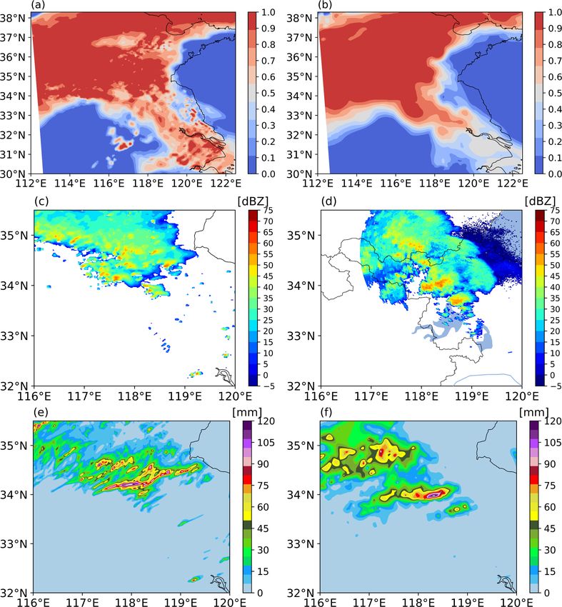
1724                        L. Kou et al.: Simulation and sensitivity analysis of spaceborne radar cloud and precipitation

mum detectable signal of about −29 dBZ. The CPR footprint             China has also begun its own spaceborne millimeter-wave
size is 1.4 km across-track and 2.5 km along-track, and the        radar project. The National Satellite Meteorological Center
vertical resolution is approximately 500 m (Stephens et al.,       plans to launch a cloud-detecting satellite, whose main load
2008). Since its launch, CloudSat CPR has obtained a large         will be the cloud-profiling radar (Wu et al., 2018). For the
quantity of cloud vertical profile data and has been widely        development of spaceborne cloud radar, simulation research
used in cloud physics, weather, environment, climatology,          on cloud and precipitation detection can provide important
and other fields (Dodson et al., 2018; Stephens et al., 2018;      theoretical support for the design and performance analysis
Battaglia et al., 2020). Spaceborne millimeter-wave radar can      of the system.
not only detect the vertical structure of various cloud systems       In this study, we quantify the uncertainty of different phys-
but also measure the distribution of snow, light rain, and even    ical model parameters for hydrometeors contributing to radar
moderate rain (Haynes et al., 2009). This provides an oppor-       reflectivity uncertainty via a sensitivity analysis and present
tunity to advance the understanding of the way water cycles        radar reflectivity simulations with optimal parameter settings
through the atmosphere by jointly observing clouds and asso-       based on forward modeling for spaceborne millimeter-wave
ciated precipitation (Behrangi et al., 2013; Ellis et al., 2009;   (94 GHz, W-band) radar. Sensitivity analyses of typical cloud
Hayden and Liu, 2018).                                             parameters on the radar equivalent reflectivity factors were
   Recently, many countries have begun research on next-           carried out. Parameters included the particle size distribution
generation spaceborne cloud radar (Battaglia et al., 2020;         (PSD) parameters, PSD model, particle density parameters,
Illingworth et al., 2015; Tanelli et al., 2018; Wu et al.,         shape, and orientation. Using appropriate physical parame-
2018), such as the CPR on the EarthCARE satellite and              ter settings, we present and compare the simulation results
dual-frequency cloud radar on the Aerosol-Cloud-Ecosystem          of two typical cloud precipitation scenarios with measured
(ACE) mission (Illingworth et al., 2015; Tanelli et al., 2018).    CloudSat results. Based on a sensitivity analysis of typical
Forward modeling and simulation play an important role             cloud parameters and a demonstration of cloud precipitation
in the design of the observation system and the interpreta-        cases, we show the radar reflectivity uncertainty caused by
tion of cloud and precipitation observation data (Horie et         the physical modeling of hydrometeors while emphasizing
al., 2012; Lamer et al., 2021; Leinonen et al., 2015; Marra        the importance of assuming more realistic scattering charac-
et al., 2013; Sassen et al., 2007; Wang et al., 2019; Wu           teristics, as well as appropriate density relations and PSD pa-
et al., 2011). QuickBeam is a user-friendly radar simula-          rameters corresponding to different cloud precipitation types.
tion package that converts modeled clouds to the equivalent
radar reflectivities measured by a wide range of meteorolog-
ical radar (Haynes et al., 2007). The Satellite Data Simulator     2     Modeling
Unit (SDSU) developed by Nagoya University, Japan, is a
satellite multisensor simulator integrating radar, microwave       2.1    Overview
radiometer, and visible and infrared imager. The Goddard
                                                                   The framework of forward modeling and simulation for
Satellite Data Simulator Unit (G-SDSU) is a derivative ver-
                                                                   spaceborne millimeter radar was composed of eight submod-
sion of the SDSU (Masunaga et al., 2010). In addition to the
                                                                   ules: cloud precipitation scene simulation with the Weather
basic functions of the SDSU, it can be coupled with high-
                                                                   Research and Forecasting (WRF) model (Skamarock et al.,
precision NASA atmospheric models, such as the Weather
                                                                   2019), WRF output result verification, hydrometeor micro-
Research and Forecasting-Spectral-Bin Microphysics (WRF-
                                                                   physical characteristic modeling, particle scattering and at-
SBM) model (Iguchi et al., 2012). The Global Precipitation
                                                                   tenuation characteristic calculations, atmospheric radiation
Measurement (GPM) satellite simulator is also based on the
                                                                   transmission calculation, output radar echo through coupling
G-SDSU, which converts the geophysical parameters simu-
                                                                   with platform and instrument parameters, sensitivity anal-
lated by the WRF-SBM into observable microwave bright-
                                                                   ysis, and comparisons and analyses of the result. Figure 1
ness and equivalent reflectivity factor signals of the GPM
                                                                   shows the logic structure between each submodule. The key
(Matsui et al., 2013). The particle shape, composition, ori-
                                                                   points of each submodule are described as follows.
entation, and mass relation all affect the scattering charac-
teristics and then influence the radar reflectivity simulation         1. From CloudSat historical data and typical weather pro-
results. The radar reflectivity for the W-band is also sensitive          cesses we obtained the cloud precipitation scene cases.
to microphysical parameters like the particle size distribution           According to the occurrence area and time, the corre-
(PSD) model and parameter, particle shape, orientation, and               sponding National Center of Environmental Prediction
mass (Mason et al., 2019; Nowell et al., 2013; Sy et al., 2020;           Final (NCEP FNL) reanalysis data were obtained as the
Wood et al., 2013, 2015). A sensitivity analysis is essential             initial field in the WRF model.
for estimating the effects of these uncertainties on simulated
radar reflectivity and guiding an appropriate parameter set-           2. The WRF model was used to simulate the distribution
ting in forward modeling.                                                 of all types of hydrometeors in these cases. In this re-
                                                                          search, we used version 4.1.2 of the advanced research

Atmos. Meas. Tech., 16, 1723–1744, 2023                                              https://doi.org/10.5194/amt-16-1723-2023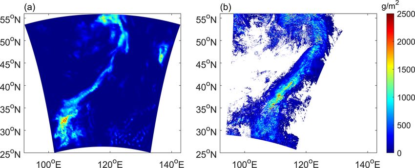
L. Kou et al.: Simulation and sensitivity analysis of spaceborne radar cloud and precipitation                                1725

      WRF model (Skamarock et al., 2019). The WRF simu-             the proportions of different components. Given the propor-
      lation results were then validated by using the real satel-   tion of air, ice, and water (or riming fraction or melting frac-
      lite and ground observation data such as ground-based         tion) in the hydrometeor, the refractive index of the mixture
      radar data.                                                   can be calculated using the Maxwell–Garnett mixing formula
                                                                    (Ryzhkov et al., 2011).
 3. Based on the hydrometeor mixing ratio of the WRF
    output and assuming certain microphysical parameters            2.2.1    Cloud water
    based on empirical information obtained from a large
    number of observation data, the PSD of the hydrome-             Cloud water droplets form from the condensation of super-
    teor particles was modeled.                                     saturated water vapor onto cloud condensation nuclei. They
                                                                    are usually spherical due to surface tension, with a typical
 4. The complex refractive index of different hydrometeors
                                                                    size of ∼ 10 µm (Mason, 1971; Miles et al., 2000). As the
    was calculated according to the particle phase and tem-
                                                                    size of cloud droplets is small relative to the wavelength, with
    perature. The scattering and attenuation characteristics
                                                                    an approximately spherical shape, their scattering character-
    of the hydrometeor particles were then calculated using
                                                                    istics can usually be calculated via Mie theory (Bohren and
    the T-matrix method (Mishchenko and Travis, 1998).
                                                                    Huffman, 1983) or Rayleigh approximation (Zhang, 2017)
    Meanwhile, the absorption coefficients of the atmo-
                                                                    based on the sphere assumption. The PSD of cloud water can
    spheric molecules, such as the water vapor and oxygen,
                                                                    generally be modeled with a normalized gamma distribution
    were calculated based on the Liebe attenuation model
                                                                    (Bringi and Chandrasekar, 2001; Chase et al., 2020):
    (Liebe, 1981).
                                                                                     (3.67 + µ)µ+4 D µ

 5. The radar reflectivity factor was then calculated based                              6
                                                                    N (D)dD =Nw
    on the atmospheric radiation transmission process and                       3.674 0(µ + 4)       D0
    the scattering and attenuation coefficients of hydrome-
                                                                                              D

    teors.                                                                   exp −(3.67 + µ)       dD,                          (1)
                                                                                              D0
 6. Through coupling with the instrument and platform pa-                 W 4 (3.67 + µ) 4

    rameters, the radar echo signal was calculated using the        Nw =                    ,                                   (2)
                                                                         π ρw (4 + µ) D0
    radar equation.
                                                                    where N (D) is the particle size distribution; D is the volume
 7. During the simulation process, the sensitivity analysis         equivalent diameter; Nw is the normalized intercept parame-
    of typical cloud physical parameters was performed to           ter; D0 is the median volume diameter; ρw is the density of
    guide the optimal microphysical modeling of the hy-             water, i.e., 1 g cm−3 ; µ is the shape parameter; and 0 is the
    drometeors.                                                     gamma function. Uniform bin sizes are set for hydrometeors,
 8. Finally, the simulation results were compared with ob-          for example dD is 0.01 mm for cloud water.
    servation data, such as CloudSat data, to validate the             Here, W in Eq. (2) is the water content of the cloud wa-
    forward simulations.                                            ter, which is calculated by converting the mixing ratio of the
                                                                    hydrometeor from the WRF output:
2.2   Hydrometeor microphysical modeling                                      P
                                                                    W=                × 1000 × q,                               (3)
                                                                            Rgas TV
The radar reflectivity factor depends on the size, shape, ori-
entation, density, size distributions, and dielectric constants     where Rgas is the specific gas constant, P is the air pressure
of the hydrometeor particles. The microphysical character-          in hectopascals, TV is the virtual temperature in K, q is the
istics of each hydrometeor are substantially different, which       mixing ratio of the hydrometeor based on the WRF output in
affects the scattering properties and also the radar echo. The      kg kg−1 , and W is g m−3 . As W is the output of the WRF
following introduces the microphysical modeling of the dif-         model, the PSD of the gamma distribution was mainly deter-
ferent hydrometeors.                                                mined by two parameters, i.e., D0 and µ. According to Miles
   The complex refractive index of each hydrometeor was             et al. (2000) and Yin et al. (2011), we simulated the PSD
first calculated, which depends on its phase, composition,          with D0 and µ ranging from 0.005–0.05 mm and 0–4 mm,
density, and radar wavelength. For pure water and pure ice,         respectively.
such as raindrops, cloud water, and cloud ice, we calculated
the refractive index according to Ray (1972). Dry snow and          2.2.2    Rain
graupel are a mixture of air and ice, while wet snow and grau-
pel are a mixture of air, ice, and water. The densities of air,     Owing to the effects of surface tension, aerodynamic force,
ice, and water are generally 0.001, 0.917, and 1 g cm−3 , re-       and hydrostatic gradient force, raindrops often take the shape
spectively. The mixture has different densities according to        of an oblate spheroid (horizontal axis (a0 ) > vertical axis

https://doi.org/10.5194/amt-16-1723-2023                                                Atmos. Meas. Tech., 16, 1723–1744, 2023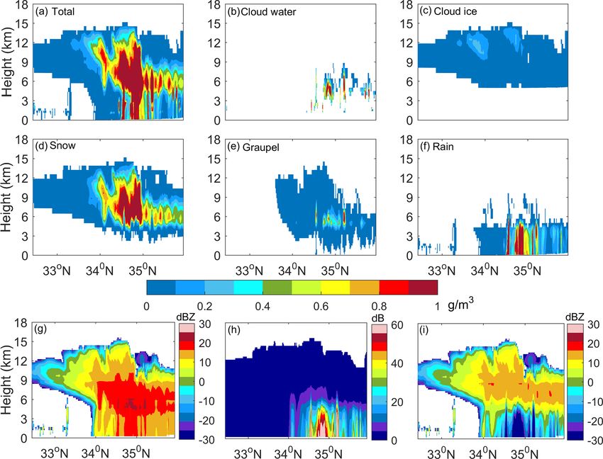
1726                        L. Kou et al.: Simulation and sensitivity analysis of spaceborne radar cloud and precipitation

Figure 1. Submodule structure and framework of the simulation model.

(b0 )), with an increase in the size of the raindrop. Here, we         can be used to examine the scattering characteristics of ice
used the axis ratio model proposed by Brandes et al. (2002):           crystals with different shapes. Here, we used the T matrix
        b0                                                             (Mishchenko and Travis, 1998) to calculate the scattering
γw =       = 0.9951 + 0.0251D − 0.03644D 2                             properties of ice crystals, which were assumed to be either
        a0
                                                                       spheroids or circular cylinders. The spheroids were treated
   + 0.005303D 3 − 0.0002492D 4 ,                           (4)        as horizontally aligned oblate spheroids with an axial ratio
                                                                       of 0.6 (Hogan et al., 2012); the relation between the larger
where D is the equivolume diameter. The scattering and at-
                                                                       and smaller dimension of the cylinders was as follows (Fu,
tenuation characteristics of raindrops were calculated using
                                                                       1996):
the T-matrix method. Considering the influence of aerody-
namics on the particle orientation, the canting angle of rain-
                                                                          L/ h = 5.068L0.586 L > 0.2 mm
drops was assumed to follow a Gaussian distribution with a                                                                      (5)
                                                                          L/ h = 2               L ≤ 0.2 mm.
mean value of 0◦ and a standard deviation (SD) of 7◦ (Zhang,
2017).                                                                 The distribution of orientations of ice particles depends
   The PSD of raindrops was still modeled as the gamma dis-            on their falling behavior. According to Melnikov and
tribution shown in Eqs. (1) and (2), where W was calculated            Straka (2013), we assume that the ice crystal orientations fol-
based on the rain mixing ratio from the WRF output. Accord-            low a Gaussian distribution, with a mean canting angle of 0◦
ing to Bringi and Chandrasekar (2001), D0 and µ were uni-              and an SD between 2 and 20◦ .
formly distributed in ranges of 0.5–2.5 mm and −1 to 4 mm,                The PSD of cloud ice is mainly represented as an exponen-
respectively.                                                          tial or gamma distribution (Ryzhkov and Zrnic, 2019). Here,
                                                                       the normalized gamma distribution was adopted according to
2.2.3    Cloud ice                                                     the empirical fits derived in Heymsfield et al. (2013). The re-
                                                                       lation between the number concentration, Nw , and D0 is as
Cloud ice is mainly composed of various non-spherical ice              follows:
crystals; the size and shape of ice crystal particles are com-
                                                                                W 4 (3.67 + µ) 4

plex and diverse, depending on the cloud temperature, the
degree of supersaturation in the environment where the par-            Nw =                          ,                             (6)
                                                                               π ρi (4 + µ) D0
ticle forms and grows, and whether the particles have experi-
enced aggregation processes in the cloud (Heymsfield et al.,           where ρi is 0.917 g cm−3 , and W is the water content of cloud
2013; Ryzhkov and Zrnic, 2019). The database in Liu (2008)             ice from the WRF output.

Atmos. Meas. Tech., 16, 1723–1744, 2023                                                 https://doi.org/10.5194/amt-16-1723-2023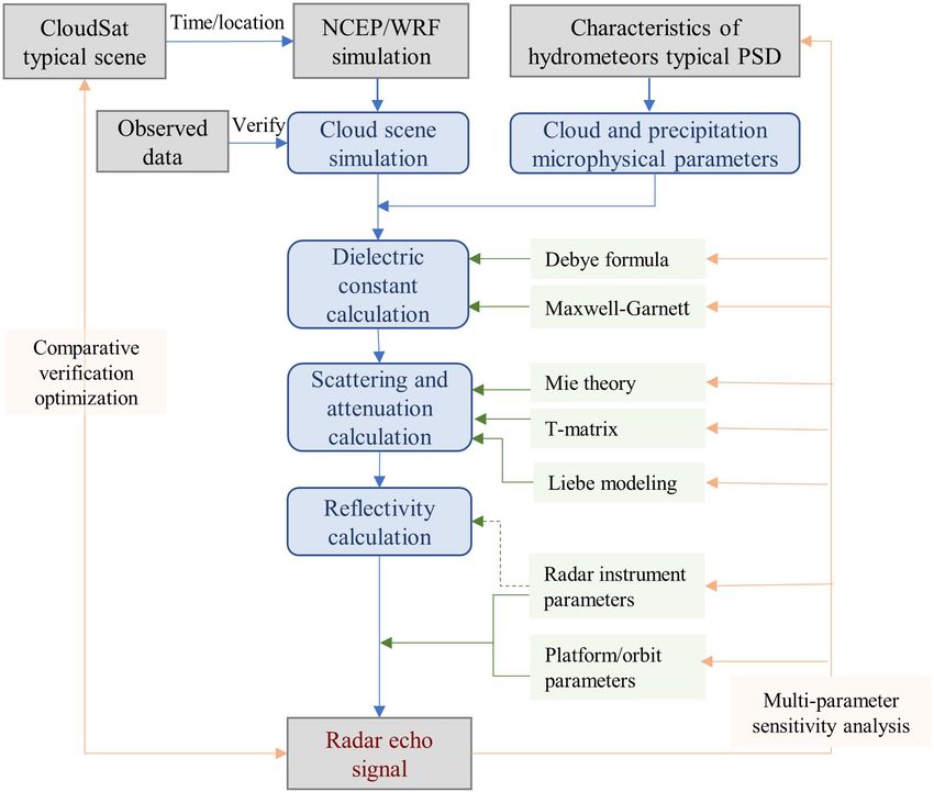
L. Kou et al.: Simulation and sensitivity analysis of spaceborne radar cloud and precipitation                              1727

  According to Heymsfield et al. (2013), the total number            Constants a and b strongly depend on the snow habit and
concentration, Nt , is a function of the temperature, T :         microphysical processes that determine snow growth and are
                                                                  usually determined experimentally. The exponent value of
        2.7 × 10⁴                           T ≤ −60 ◦ C

Nt =                                                      (7)     b is generally a Gaussian distribution, with a mean of 2.1
                     3
        3.304 × 10 exp (−0.04607T ) T > −60 ◦ C.                  (Brandes et al., 2007; Heymsfield et al., 2010; Szyrmer and
                                                                  Zawadzki, 2010; von Lerber et al., 2017). The prefactor a
The maximum diameter, Dmax , is also dependent on T :             can vary considerably, and the value of a increases with

         11 exp (0.069T ) stratiform                              the aggregate density or riming degree (Huang et al., 2019;
Dmax =                                                (8)         Ryzhkov and Zrnic, 2019; Sy et al., 2020; Wood et al., 2015).
         21 exp (0.070T ) convective,
                                                                  Most of the mass and density relations in previous studies
where T is in degrees Celsius, Nt is in cubic meters, and         (Brandes et al., 2007; Sy et al., 2020; Szyrmer and Zawadzki,
Dmax is in millimeters. Given T and the water content of          2010; Tiira et al., 2016) showed that the prefactor a varies
cloud ice, W , as well as the empirical value of µ, we can cal-   between 0.005 and 0.014 cgs units (i.e., in g cm−b ), where D
culate D0 from Eqs. (1), (6)–(8), and the following formula:      and m are in centimeters and grams; the mean value is ap-
                                                                  proximately 0.009. In different studies, the statistical results
        D
        Zmax                                                      of mass–size relations vary slightly (Brandes et al., 2007;
Nt =            N (D)dD.                                   (9)    Mason et al., 2018; Tiira et al., 2016; Wood et al., 2015), with
            0
                                                                  the primary difference being the diameter expression for the
                                                                  maximum dimension diameter, Dm ; median volume diame-
Owing to the monotonicity of the functions, D0 can be solved      ter, D0 ; or volume equivalent diameter, D. In this study, the
numerically. For cloud ice, µ usually ranges from 0 to 2          diameters in the mass and density relations were converted to
(Tinel et al., 2005; Yin et al., 2011).                           the volume equivalent diameter D according to the assumed
                                                                  axis ratio.
2.2.4       Snow
                                                                  2.2.5   Graupel
Snowflakes are usually formed by the aggregation and
growth of ice crystals. Although the shapes of snowflakes         Graupel is generated in convective clouds by the accretion of
are irregular, they can also be modeled as spheroids, with        supercooled liquid droplets on ice particles or by the freez-
a constant axis ratio of 0.75 (Zhang, 2017). For large snow       ing of supercooled raindrops lofted in updrafts. The density
aggregates, an axis ratio of approximately 0.6 is regarded        of graupel varies substantially depending on their formation
as a good model, especially for explaining multifrequency         mechanism, time of growth from the initial embryo, liquid
radar observations (Matrosov, 2007; Moisseev et al., 2017).       water content, and ambient temperature. The density is gen-
As snowflakes fall with their major axis mainly aligned in        erally between 0.2 and 0.9 g cm−3 , with a typical value of
the horizontal direction, the mean canting angle of snow is       approximately 0.4 g cm−3 from the statistical results in ob-
assumed to be 0◦ , and the SD of the canting angle is assumed     servation experiments (Heymsfield et al., 2018; Ryzhkov and
to be 20◦ (Zhang, 2017). The width of the canting angle dis-      Zrnic, 2019).
tribution grows with an increase in aggregation. Garrett et          Generally, graupel particles have irregular shapes. Here
al. (2015) showed that the average SD of moderate-to-heavy        the shape of graupel was modeled as a spheroid, where the
snow, consisting of dry aggregates, is approximately 40◦ .        axis ratio for dry graupel was set to a constant value of 0.8,
   The PSD of snow is modeled as an exponential distribu-         and the axis ratio for melting graupel was modeled according
tion; the distribution parameters are constrained by the mass–    to Ryzhkov et al. (2011) as
power function relationship (Kneifel et al., 2011; Lin and
Colle, 2011; Matrosov, 2007; Tomita, 2008; Woods et al.,          γg = 0.8   fw ≤ 0.2
2008):                                                            γg = 0.88 − 0.4fw      0.2 < fw < 0.8
                                                                  γg = 2.8 − 4γw + 5 (γw − 0.56) fw       fw ≥ 0.8,          (13)
N(D)dD = N0 exp(−3D)dD,                                   (10)
                                         6                        where γw is the axis ratio of raindrops, and fw is the mass
m(D) = aD b ,        or ρs (D) =           aD b−3 ,       (11)    water fraction. The SD of the canting angle, δ, was parame-
                                         π
                              1                                 terized as a function of fw :
            aN0 0(b + 1)       b+1
3=                                   ,                    (12)
                 W                                                δ = 60◦ (1 − cfw ) ,                                       (14)

where N0 is the intercept parameter (usually ranging between      where c is an adjustment coefficient, usually set as 0.8 (Jung
103 –105 mm−1 m−3 ); D is the volume equivalent diameter;         et al., 2008).
and m(D) and ρs (D) are the mass and density of the particle,        The PSD of graupel is assumed to be an exponential dis-
respectively.                                                     tribution, as shown in Eqs. (10)–(12). In convective clouds,

https://doi.org/10.5194/amt-16-1723-2023                                            Atmos. Meas. Tech., 16, 1723–1744, 2023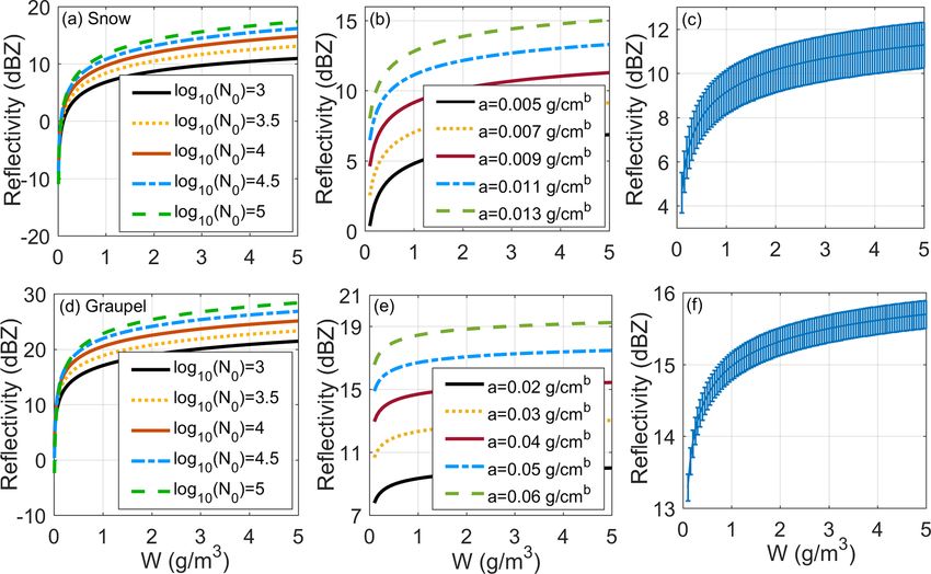
1728 L. Kou et al.: Simulation and sensitivity analysis of spaceborne radar cloud and precipitation
a large part of graupel likely develops via collisions be- According to the mass conservation model, the total liquid
tween frozen drops and smaller droplets, and its bulk den- water content of a distribution is conserved. The number con-
sity decreases with increasing graupel size (Khain and Pin- centration of raindrops (Nw ) in each size is calculated as fol-
sky, 2018). Similar mass relations can be found for graupel, lows:
and its exponent b is larger than that for snow. The expo-
1
nent for low-density graupel is approximately 2.3 (Erfani and 3 6 − 3 3−b
Mitchell, 2017; von Lerber et al., 2017), while that for lump Nw (Dw ) = Nms (Dms ) a Dms3 , (19)
b π
graupel approaches 3.0 (Mace and Benson, 2017; Mason et
al., 2019). The mean value of b is approximately 2.6, and where Nms (Dms ) is the number concentration of melting par-
prefactor a varies mainly between 0.02 and 0.06 g cm−b (Ma- ticles.
son et al., 2018; Heymsfield et al., 2018), where the units for The scattering characteristics of melting particles are still
m and D are grams and centimeters. calculated by the T matrix. It is assumed that the shape of
melted ice particles gradually changes with the increase of
2.2.6 Melting modeling
mass water fraction fw , so as to finally obtain the shape of
Neglecting aggregation, collision–coalescence, evaporation, raindrops with the same mass. We can introduce the axis ra-
and the small amount of water that may collect on the particle tio (γms ) relationship and the relationship of the SD of the
owing to vapor diffusion, we assume that the mass of snow canting angle (δmr ) for melting particles as (Ryzhkov and Zr-
was conserved during the evolution process from dry snow nic, 2019)
to wet snow to liquid water:
3 3
γms = γs + fw (γw − γs )
ρw D w = ρms Dms = ρs Ds3 , (15)
δms = δs + fw (δr − δs ) , (20)
where ρw , ρm , and ρs are the densities of the liquid water
and melting and dry particles, respectively; Dw , Dms , and where γs is the axis ratio of dry snow; γw is the axis ratio of
Ds are the diameters of water, melting snow, and dry snow, the raindrop, which is produced as a result of snow melting;
respectively. and δr is the SD of the canting angle distribution of raindrops,
If the mass fraction of melt water in the particle of fw whereas δs is the corresponding SD of the distribution of dry
is known, the density of melting snow can be obtained as snow.
follows (Haynes et al., 2009):
ρs ρw 2.3 Radar equation
ρms = . (16)
fw ρs + (1 − fw ) ρw
The density of snowflakes follows the power-law relation The signal power, Pr , received by the radar was calculated
in Eq. (11). The density parameter in Eq. (11) can be ob- using the radar equation:
tained according to the density–diameter relationship, where
Zr0
the density is calculated from Eq. (16) with an assumed fw Pt
value. The dielectric constant of melting snow depends on Pr = C 2 Ze exp −2 k(r)dr , (21)
r0
snow density and water fraction fw . Here, we use the model 0
that water is considered background, and snow is treated as
inclusions, and we compute the dielectric constant based on where Pt is the transmitted power, r0 is the range to the at-
Maxwell–Garnett formulas for the mixture of snow and wa- mospheric target, C is the radar constant related to the instru-
ter (Ryzhkov et al., 2011; Zhang, 2017). ments, and k is the attenuation coefficient. The radar equiva-
According to Eqs. (11) and (15), the relation between the lent reflectivity factor, Ze , was calculated from the scattering
particle diameters can be obtained as follows: characteristics and the assumed PSD of the various hydrom-
1 b eteors:
6 3
3
Dw = a Dms , (17) Z∞
π λ4
Ze = 5 N (D)σb (D)dD, (22)
where the mass-equivalent melted diameter Dms correspond- π |Kw |2
ing to diameter Ds of each dry snow particle is calculated 0
from Eq. (15).
Due to melting, the uniform bin size set no longer applies, where σb (D) is the backscattering cross section of the par-
such that a new bin size must be calculated. The bin size for ticle with a diameter D; λ is the radar wavelength; and
rain (dDw ) can be obtained by differentiating as follows: Kw = (n2w − 1)/(n2w + 2), where nw is the complex refractive
index of water for a given wavelength and temperature.
1 b−3
b 6 3 For spaceborne millimeter-wave radar, the equivalent
dDw = a Dms3 · dDms . (18) radar reflectivity factor (hereafter radar reflectivity) observed
3 π
Atmos. Meas. Tech., 16, 1723–1744, 2023 https://doi.org/10.5194/amt-16-1723-2023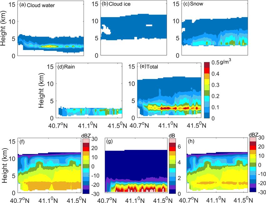
L. Kou et al.: Simulation and sensitivity analysis of spaceborne radar cloud and precipitation 1729
by the radar is the attenuated radar reflectivity factor, Ze0 :
Zr0
Ze0 = Ze exp −2 k(r)dr ,
0
Z
k = 10−3 Qt (D)N (D)dD, (23)
where the units of k are 1 km−1 , Qt (mm2 ) is the extinction
cross section of the corresponding hydrometeor calculated by
the T matrix, the units of N (D) are m−3 mm−1 , and the unit
of dD is millimeters. During radar reflectivity calculation, a
look-up table of backscattering and extinction cross sections
is established for reducing the calculation workload.
If there are many types of hydrometeors at the same height,
the equivalent unattenuated radar reflectivity and attenuation
coefficient of each hydrometeor is calculated based on the
look-up table. Then, the total unattenuated radar reflectivity Figure 2. Impact of the PSD parameters, i.e., D0 and µ, on radar
at this height is obtained by adding all types of hydrome- reflectivity for cloud water and rain. Reflectivity variation in cloud
teors, and the two-way attenuation is obtained by integrat- water caused by (a) a D0 of 10, 20, 30, 40, and 50 µm with a µ of
1 and (b) µ values of 0, 1, and 2 with a D0 of 20 µm. Reflectivity
ing the total attenuation coefficient with path. The attenuated
variation in rain caused by (c) a D0 of 0.5, 1, 1.5, 2, and 2.5 mm
radar reflectivity is obtained by subtracting the attenuation with a µ of 3 and (d) µ values of −1, 0, 1, 2, 3, and 4 with a D0 of
from the unattenuated radar reflectivity. Considering the dif- 1.25 mm.
ference between the resolution of the simulation data and the
observation resolution of the instrument, the convolution of
the simulation echo and antenna pattern was also performed the gamma PSD parameters for cloud water and rain. Cloud
during the coupling process of the simulation data and in- water particles are small compared to the radar wavelength,
strument parameters. During this process, the antenna pattern which is in the linear growth stage in the Mie scattering re-
was set as a two-dimensional Gaussian distribution. gion. With a 5-fold increase in D0 (W remains constant), e.g.,
After coupling with the antenna pattern, the final radar re- increasing from 10 to 50 µm, the reflectivity increases by ap-
flectivity was obtained. Here, the unit of Ze is mm6 m−3 , proximately 20 dB. For rain particles, the impact of D0 is
and it is usually expressed in decibel form as dBZe = 10 × not as significant as that of cloud water: a 5-fold change in
log10 (Ze ). D0 can lead to a reflectivity change within 5 dB. Owing to
the Mie scattering effect on raindrops, the contribution from
relatively small raindrops may be more than that from larger
3 Sensitivity analysis
raindrops considering the influence of the number concentra-
Due to complex microphysical processes in cloud precipi- tion. In the gamma PSD, the effect of µ is relatively small;
tation, the PSDs of hydrometeors vary substantially. An ac- the reflectivity change caused by µ is within 1.5 dB when
curate PSD is difficult to measure, especially for aloft parti- using a constant D0 .
cles. The phase, size, and shape of particles also change with For cloud ice, D0 is calculated from Eqs. (6)–(9) given W
the dominating microphysical processes and external envi- and T ; µ is the only parameter that needs to be assumed.
ronment, which all affect the simulation results. For optimiz- Figure 3a and b show the reflectivity change with W and µ,
ing the parameter settings of the forward modeling and more where Fig. 3a was obtained when T was −20 ◦ C, and Fig. 3b
accurately interpreting the radar reflectivity results, we per- was obtained when T was −60 ◦ C. As the PSD of cloud ice
formed a series of sensitivity analyses of cloud parameters. was constrained by the total number concentration, D0 and
Here, we mainly focused on the scattering effects; the atten- µ are interrelated, and D0 increases with an increase in µ,
uation effects will be discussed in a follow-up study. W , and T . Based on Fig. 3a and b, we observed that when
µ varies from 0 to 2, the maximum reflectivity change is
3.1 PSD parameters approximately 4 dB at −20 ◦ C, while that at −60 ◦ C is ap-
proximately 5 dB. The reflectivity change was still affected
The gamma distribution is determined by three parameters. by the D0 variation. Based on Eqs. (6)–(9), D0 varied from
As one of the parameters is obtained from the water content, 0.1–0.5 mm at −60 ◦ C and 0.2–0.8 mm at −20 ◦ C when W
W , of the hydrometeor in the WRF output, we mainly con- ranged from 0 to 0.5 g m−3 . Figure 3c and d show the re-
sidered the effects of D0 and µ on the radar reflectivity. Fig- flectivity change caused by D0 and µ under a conventional
ure 2 shows the radar reflectivity change with variations in gamma PSD without constraints on the total number con-
https://doi.org/10.5194/amt-16-1723-2023 Atmos. Meas. Tech., 16, 1723–1744, 2023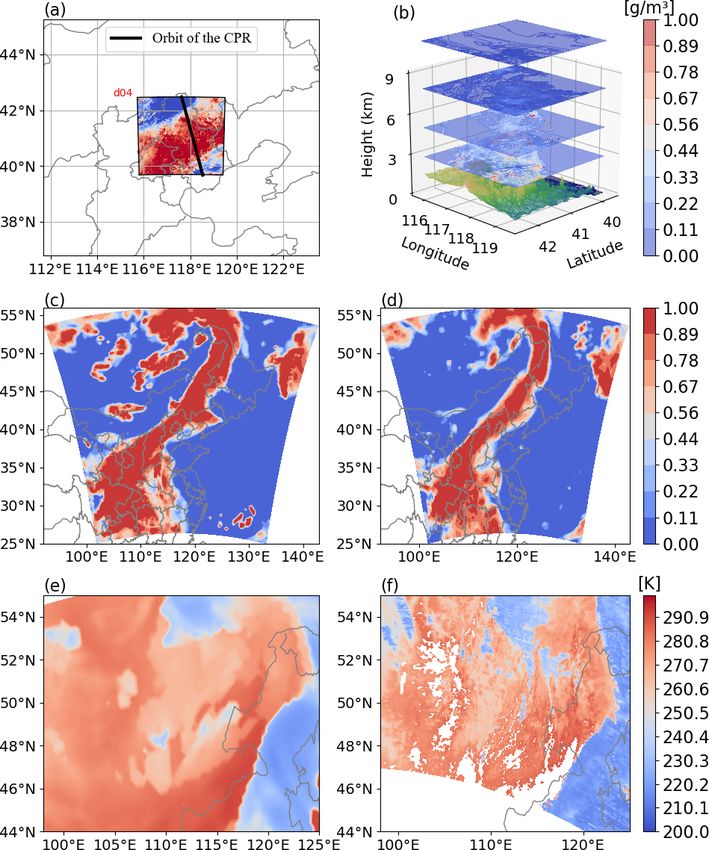
1730                          L. Kou et al.: Simulation and sensitivity analysis of spaceborne radar cloud and precipitation

                                                                        rived the mean value of b to be close to 2.1 via averaging
                                                                        literature values of b from the list of studies (Brandes et al.,
                                                                        2007; Heymsfield et al., 2010; Huang et al., 2019; Sy et al.,
                                                                        2020; Szyrmer and Zawadzki, 2010; Tiira et al., 2016; Wood
                                                                        et al., 2013). For graupel, the exponent b varies from 2.1 to
                                                                        3, and a mean value of approximately 2.6 was derived from
                                                                        the studies in the literature (Heymsfield et al., 2018; Mason
                                                                        et al., 2018; Von Lerber et al., 2017). Based on the range and
                                                                        mean value of b for the Gaussian distribution, we calculated
                                                                        the standard deviation (SD) to be 0.28 and 0.16 for snow and
                                                                        graupel, respectively. The error bars in Fig. 4c and f repre-
                                                                        sent the SD of the reflectivity change caused by variation in
                                                                        b, which was approximately 2 dB for snow and 0.5 dB for
                                                                        graupel. The results showed that the sensitivity of reflectivity
                                                                        to prefactor a was substantially greater than that to exponent
                                                                        b.
                                                                           All in all, the mass relationships that depend on par-
Figure 3. Impact of PSD parameters on radar reflectivity for cloud      ticle habits and formation mechanisms cause substan-
ice. PSD parameters constrained by Eqs. (7)–(9); reflectivity vari-     tial uncertainties in W-band radar reflectivity. Our results
ation obtained when µ was 0, 1, and 2 and (a) temperature T was         are consistent with the sensitivity analysis by Wood and
−20 ◦ C and (b) T was −60 ◦ C. PSD parameters varied indepen-
                                                                        L’Ecuyer (2021), who pointed out that the W-band radar re-
dently; reflectivity variation obtained by a (c) D0 of 0.1, 0.2, 0.4,
                                                                        flectivity uncertainty for snowfall was dominated by the par-
0.6, 0.8, and 1 mm with a µ of 1 and (d) µ values of 0, 1, and 2 with
a D0 of 0.2 mm.                                                         ticle model parameter (e.g., the prefactors and exponents of
                                                                        the mass relationships). The mass relationship can cause the
                                                                        reflectivity uncertainty of several to more than 10 dB. The re-
                                                                        sults indicate that improved constraints on assumed particle
centration. In the conventional gamma PSD, D0 and µ vary                mass models would improve forward-modeled radar reflec-
independently; the reflectivity can change by 13 dB when D0             tivity and physical parameter retrieval.
varies from 0.2 to 0.8 mm. The results showed that the ef-
fect of PSD parameter variation on the reflectivity can be re-          3.2   PSD models
duced by approximately 60 %, owing to constraints on the
total number concentration for the PSD of cloud ice.                    The PSDs of hydrometeors can usually be represented by dif-
   An exponential PSD with a power-law mass spectrum was                ferent distributions, such as the gamma distribution and log-
used for snow and graupel. Figure 4 shows the effects of in-            normal distribution, which are frequently used in cloud water
tercept parameter N0 and the mass power-law parameters of               PSDs. This section discusses the influence that the selection
prefactor a and exponent b. With the mean mass–size rela-               of different PSD models has on the radar reflectivity factor,
tionships for snow and graupel, changing the log10 (N0 ) from           taking cloud water as an example. Figure 5a shows two PSD
3 to 5 could cause a reflectivity increase of approximately             models of cloud water in which the solid black line repre-
7–8 dB, as shown in Fig. 4a and d.                                      sents the gamma distribution, and the dotted red line repre-
   The mass power-law parameters vary with snow and grau-               sents the lognormal distribution. The lognormal distribution
pel type, shape, and porosity. In Fig. 4b and e, we see that            uses the following formula (Miles et al., 2000):
with a constant N0 and mean value of exponent b, the reflec-                               6W

                                                                                                             9 2

tivity change caused by variation in prefactor a from 0.005             N (D)dD = √                  exp − σ
                                                                                      π 2π ρp σ Dm 3         2
to 0.013 g cm−b for snow and 0.02 to 0.06 g cm−b for grau-                               "                    #
pel (W remains constant) can reach 7–10 dB. An increase in                                   (ln D − ln Dm )2 dD
a leads to an obvious increase in the corresponding particle                         exp −                         ,             (24)
                                                                                                    2σ 2        D
scattering properties and then causes the reflectivity change.
Using an average mass–power relation assumption, the vari-              where Dm is the mass-weighted diameter, and σ is the dis-
ation in a as a result of the degree of aggregation and riming          persion parameter.
and particle shapes may result in the reflectivity uncertainty             The parameters in the PSD model in Fig. 5a are based on
of approximately 45 % and 30 % for snow and graupel, re-                the parameter settings for cloud water in terrestrial stratiform
spectively. For analyzing the effect of the variation in b, a           clouds (Mason, 1971; Miles et al., 2000; Niu and He, 1995),
Gaussian distribution of b was modeled. According to re-                where D0 is 20 µm, µ is 2 in the gamma distribution, Dm is
sults from observation experiments reported in the literature,          20 µm, σ is 0.35 in the lognormal distribution, and W in both
the exponent b for snow varies from 1.4 to 2.8, and we de-              PSD models is set to 1 g m−3 . The solid black line represents

Atmos. Meas. Tech., 16, 1723–1744, 2023                                                  https://doi.org/10.5194/amt-16-1723-2023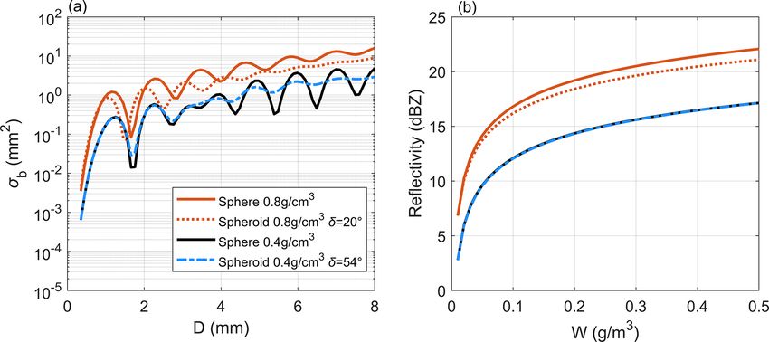
L. Kou et al.: Simulation and sensitivity analysis of spaceborne radar cloud and precipitation                                            1731

Figure 4. Impact of PSD parameters on radar reflectivity for snow and graupel. Variation in reflectivity for snow at (a) log10 (N0 ) values
of 3, 3.5, 4, 4.5, and 5 with a mean mass–diameter relationship of m = 0.009D 2.1 , where D is in centimeters, and m is in grams; (b) pref-
actor a in a mass–diameter relationship of 0.005, 0.007, 0.009, 0.011, and 0.013 g cm−b , with exponent b of 2.1 and N0 assumed to be
3 × 10³ m−3 mm−1 ; (c) mean value ± standard deviation of b, where the mean is 2.1, and the standard deviation (SD) is 0.28, with a as-
sumed to be 0.009. The vertical bars represent the SD of the reflectivity change caused by deviation from the mean value of b. Variation in
reflectivity for graupel at (d) log10 (N0 ) values of 3, 3.5, 4, 4.5, and 5 with a mean mass–diameter relationship of m = 0.04D 2.6 , where D is
in centimeters, and m is in grams; (e) prefactor a in a mass–diameter relationship of 0.02, 0.03, 0.04, 0.05, and 0.06 g cm−b , with exponent
b of 2.6 and N0 assumed to be 4 × 10³ m−3 mm−1 ; and (f) mean value ± standard deviation of b, where the mean is 2.6, and the standard
deviation is 0.16, with a assumed to be 0.04. For a and b we took literature values from a list of studies and calculated the mean, and the
standard deviation of b for snow and graupel is calculated according to the range and average of the Gaussian distribution.

                                                                          3.3    Particle shape and orientation

                                                                          The scattering properties of particles are sensitive to the hy-
                                                                          drometeor shape and orientation. Previous studies (Marra et
                                                                          al., 2013; Masunaga et al., 2010; Seto et al., 2021; Wang
                                                                          et al., 2019) often assume that the hydrometeor particle is
                                                                          a sphere, but most particles are non-spherical. This section
                                                                          discusses the influence that cloud ice, snow, graupel, and rain
                                                                          particle shapes (cloud water is generally spherical) have on
Figure 5. Impact of PSD models on radar reflectivity for cloud
water. (a) Solid black line is for the gamma distribution: W =
                                                                          radar reflectivity.
1 (g m−3 ), D0 = 20 µm, and µ = 2. Dotted red line is for the                Figure 6 compares the backscattering cross section and
lognormal distribution: W = 1 g m−3 , Dm = 20 µm, and σ = 0.35.           corresponding radar reflectivity under different shapes of
(b) Variation in the radar reflectivity with W and the PSD models,        cloud ice, dry snow, and rain. Three shape types, i.e., sphere,
where the PSD models are from (a).                                        spheroid, and cylinder, for cloud ice were considered, where
                                                                          the shape parameter setting refers to Sect. 2.2.3. The solid
                                                                          and dotted lines in Fig. 6a indicate that the SD of the cant-
the gamma distribution, and the dotted red line represents                ing angle (δ) is 2 and 20◦ , respectively. The backscatter-
the lognormal model. Corresponding to the typical param-                  ing difference for cloud ice was evident between the sphere
eter settings of the gamma and lognormal distributions, the               and non-sphere when the diameter was greater than 1 mm.
difference between the two PSDs was notable; the reflectiv-               The radar reflectivity factor in Fig. 6b was obtained with
ity change caused by the different PSD models was approx-                 the constrained PSD parameter (Sect. 2.2.3) of T = −60 ◦ C
imately 4.5 dB. This result showed that the PSD model had                 and µ = 1, and the maximum diameter was calculated ac-
a certain impact on echo simulation, and it was necessary to              cording to Eq. (8) that was within 0.4 mm. Figure 6b shows
carefully select the PSD model and set the parameters ac-                 that the spherical and non-spherical assumption for cloud ice
cording to the type of cloud and precipitation.                           may result in an average reflectivity difference of approxi-

https://doi.org/10.5194/amt-16-1723-2023                                                      Atmos. Meas. Tech., 16, 1723–1744, 2023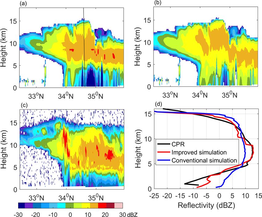
1732                        L. Kou et al.: Simulation and sensitivity analysis of spaceborne radar cloud and precipitation

mately 8 %. The reflectivity difference caused by δ was ap-
proximately 1 %. Figure 6c shows the backscattering cross
section of dry snow with a mass–diameter relation of m =
0.0075D 2.05 (Matrosov, 2007; Moisseev et al., 2017), where
the axis ratio of the spheroid was 0.6, and the SD of the cant-
ing angle was assumed to be 20 and 40◦ . When calculating
the radar reflectivity factor, the corresponding exponential
distribution parameter was N0 = 3 × 10³ m−3 mm−1 , and the
reflectivity difference between the sphere and spheroid can
reach approximately 1.6 dB. In particular, the average reflec-
tivity difference reached 14 % for a δ of 20◦ and 12 % for a δ
of 40◦ . For raindrops, the backscattering difference became
apparent after the equivalent diameter was 2 mm, as shown in
Fig. 6e. The reflectivity in Fig. 6f was obtained with a gamma
PSD parameter of D0 = 1.25 mm and µ = 3. The reflectivity
difference caused by the particle shape was negligible. This
is because particles less than 2 mm mostly contribute to the
radar reflectivity for rain. The influence of shape on raindrops
can be negligible.
   The axis ratio and particle orientation change with varia-
tions in the density of snow and graupel. Figure 7 compares
backscattering and corresponding radar reflectivity for grau-
pel between spheres and spheroids at different densities and
orientations. The SD of the canting angle in Fig. 7a was cal-
culated according to Eq. (14). Here, δ was 54◦ at a density of
0.4 g cm−3 , while δ was 20◦ at a density of 0.8 g cm−3 . Based
on Fig. 7a, the backscattering section difference increased        Figure 6. Backscattering cross section and corresponding radar re-
with density, which may have been due to the stronger refrac-      flectivity under different shapes for cloud ice, dry snow, and rain.
tive index. Figure 7b shows the corresponding radar reflectiv-     (a) Comparison of the backscattering cross sections of ice crys-
ity for particles in Fig. 7a, where the PSD was assumed to be      tals as spheres, spheroids, or cylinders, where δ is the SD of the
an exponential distribution with N0 of 4 × 10³ m−3 mm−1 .          canting angle. (b) Radar reflectivity comparison for particles in
The spherical assumption may cause an average overestima-          (a), where the PSD was assumed to be a gamma distribution con-
tion of the reflectivity by approximately 6 % when the density     strained by Eqs. (7)–(9), with µ = 1 and T = −60 ◦ C. (c) Compar-
is 0.8 g cm−3 and δ is 20◦ , whereas the reflectivity difference   ison of the backscattering cross sections for dry snow with spheres
is negligible at a δ of 54◦ and density of 0.4 g cm−3 . This re-   and spheroids. (d) Radar reflectivity comparison for particles in (c),
                                                                   where the PSD was assumed to be an exponential distribution with
sult showed that besides particle shape, the particle density
                                                                   N0 = 3 × 10³ m−3 mm−1 . (e) Comparison of backscattering cross
and orientation should also be considered in the scattering        sections for raindrops with spheres and spheroids. (f) Radar reflec-
simulation. Here we mainly discuss the backscattering dif-         tivity comparison for particles in (e), where the PSD was assumed
ference between spheres and spheroids. In future research,         to be a gamma distribution with D0 = 1.25 mm and µ = 3.
we will consider more realistic variations in particle shapes
to evaluate the sensitivity of the scattering properties to hy-
drometeor shapes more comprehensively.                             cle shapes, melting modeling, and mass–power relations for
                                                                   snow and graupel. The cases were selected by combining his-
                                                                   torical CloudSat data and typical weather processes observed
4   Simulation results for typical cases                           on the ground. For comparison, the results with a conven-
                                                                   tional simulation were also shown.
Based on the sensitivity analysis of typical cloud physical pa-
rameters, we simulated the radar reflectivity of typical cloud     4.1     Stratiform case
scenes by assuming appropriate physical parameters for dif-
ferent hydrometeors and cloud precipitation types with the         4.1.1    WRF scenario simulation
hydrometeor mixing ratio from the WRF as input. The simu-
lation results were compared with CloudSat observation data.       From 24 to 25 September 2012, there was a large-scale low
   Two typical weather cases of a cold-front stratiform cloud      trough cold-front cloud system in northwest China, which
and a deep convective process were shown, which were               moved from the west to the east and entered Shanxi Province.
simulated with improved settings, accounting for the parti-        The CloudSat satellite observed the stratiform cloud pro-

Atmos. Meas. Tech., 16, 1723–1744, 2023                                               https://doi.org/10.5194/amt-16-1723-2023
L. Kou et al.: Simulation and sensitivity analysis of spaceborne radar cloud and precipitation 1733
Figure 7. Comparison of the backscattering cross section and corresponding radar reflectivity for graupel between spheres and spheroids at
different densities and orientations. (a) Backscattering cross section at a density of 0.4 and 0.8 g cm−3 with δ (SD of canting angle) calculated
from Eq. (14). After calculation, δ was 54◦ at a density of 0.4 g cm−3 , while δ was 20◦ at a density of 0.8 g cm−3 . (b) Radar reflectivity for
particles in (a), where the PSD was assumed to be an exponential distribution with N0 of 4 × 10³ m−3 mm−1 . Overestimation caused by the
spherical assumption increased with an increase in density and decrease in δ.
cess from 40.67◦ N, 118.22◦ E to 41.56◦ N, 117.93◦ E at MODIS observations. Both exhibited low cloud-top temper-
04:23 UTC on 25 September 2012. Centered on the obser- atures in the northeast and high cloud-top temperatures in
vation range of CloudSat, this stratiform cloud process was the south. The value, location, and distribution of cloud-top
simulated by the WRF model. This experiment adopted a temperatures simulated by the WRF were consistent with the
one-way scheme with a quadruple nested grid. From the in- satellite observations.
side to the outside, the horizontal resolution was 1, 3, 9, and
27 km. It was divided into 40 layers vertically, and the top 4.1.2 Experiment design
of the model was 50 hPa. More details about the model setup
can be found in Appendix A. For comparison with CloudSat data, the two-dimensional hy-
Figure 8a shows the simulation area for the two interior drometeor profile from the WRF model on the track match-
domains (d03 and d04) in which the black line is the tra- ing CloudSat was selected as the input for the radar reflectiv-
jectory of the CloudSat CPR. Figure 8b shows the three- ity simulation. The WRF data at 04:30 UTC were selected.
dimensional distribution of the total hydrometeor output Owing to the uneven output height layer of the WRF, data
of the WRF corresponding to the innermost grid. The hy- for the WRF simulation results were interpolated in the ver-
drometeors were cloud water, snow, cloud ice, and rain. tical direction. The vertical grid of the interpolated data was
The hydrometeors were mainly distributed below 10 km; the 240 m, corresponding to the CloudSat CPR data.
maximum total water content was at approximately 3 km, Figure 9a–e show the latitude–height cross section of the
∼ 0.9 g m−3 . hydrometeors in the stratiform case simulated by the WRF
Figure 8c–f compare the fraction of cloud cover and cloud- for cloud water, cloud ice, snow, rain, and the total hydrome-
top temperature simulated by the WRF with the European teors. The vertical extent of snow is widely distributed, rang-
Centre for Medium-Range Weather Forecasts reanalysis 5 ing from 3 to 10 km. Rain is mainly below 3 km, with water
(ERA5) data (Hersbach et al., 2020) and the Moderate Res- contents between 0.1 and 0.2 g m−3 . At approximately 0 ◦ C,
olution Imaging Spectrometer (MODIS) observation data the water content for cloud water, snow, and rain was large,
(Menzel et al., 2008). The level-2 cloud product of cloud-top which led to a high total water content, with a maximum of
temperature from MODIS with spatial resolutions of 5 km 0.57 g m−3 .
was used. Considering the resolution of ERA5 data (0.25◦ ) Besides the comparison with the CloudSat observation
and the MODIS scanning track (2330 km), the outermost grid data, the simulation results with improved and conventional
in the WRF simulation data was used for comparison. Fig- settings were compared as well. For the stratiform case, the
ure 8c and d show the fraction of cloud cover from the WRF PSD parameters were assumed based on the empirical val-
model and ERA5 data, respectively. The WRF simulates the ues of land stratiform precipitation clouds (Mason, 1971;
northeastern and southwestern zonal distribution of the cold- Niu and He, 1995; Yin et al., 2011) in which the D0 of
front cloud system; the simulated cloud area and cloud cover- cloud water was set to 0.01 mm, the D0 of cloud ice was
age are consistent with the ERA5 data. Figure 8e and f com- 0.02 mm, and µ was set as a constant of 1. As snow in strati-
pare the cloud-top temperature from the WRF simulation and form clouds was mainly unrimed particles in middle and low
latitudes (Yin et al., 2017), a mass–power relation represen-
https://doi.org/10.5194/amt-16-1723-2023 Atmos. Meas. Tech., 16, 1723–1744, 20231734 L. Kou et al.: Simulation and sensitivity analysis of spaceborne radar cloud and precipitation
Figure 8. Simulation area exhibition of the stratiform cloud case scenario and comparison between the WRF model results and observation
data. (a) Exhibition of the internal two-layer simulation area, (b) three-dimensional distribution of the total hydrometeor output from the
WRF, (c) fraction of cloud cover from the WRF model, (d) fraction of cloud cover from the ERA5 data, (e) WRF model-simulated cloud-top
temperature, and (f) MODIS-observed cloud-top temperature.
tative m = 0.0075D 2.05 of unrimed snow (Moisseev et al., 4.1.3 Radar reflectivity simulation results
2017) was used in the simulation, where D was the volume
equivalent diameter. During a simulation with an improved Figure 9f–h show the simulated radar reflectivity with the
microphysical setting, a melting layer with a width of 1 km total hydrometeors, where Fig. 9f shows the unattenuated re-
was assumed below 0 ◦ C based on the statistical median of flectivity, Fig. 9g shows the two-way attenuation, and Fig. 9h
the melting layer width in stratiform precipitation observed shows attenuated reflectivity. The reflectivity above 8 km was
by radars (Liu and Zhou, 2016; Wang et al., 2012), and the mainly a result of weak cloud ice and dry snow, which did
PSD parameters of the raindrops were calculated according not exceed −5 dBZ. The radar reflectivity caused by snow
to the melting model. For the conventional setting, the melt- increased with an increase in the water content, up to approx-
ing model was not included, and the PSD parameters for rain- imately 10 dBZ. Melting led to an increase in the refractive
drops were set as D0 = 1 mm and µ = 3 based on the statisti- index and density of snow, which resulted in a sharp increase
cal average values of microphysical parameters of stratiform in the radar reflectivity. The unattenuated radar reflectivity
precipitation in eastern China (Chen et al., 2013; Wen et al., in the melting layer was equivalent to the reflectivity in the
2020). rain region. With attenuation, the radar reflectivity showed a
rapid signal decline below the melting layer, and the bright
band became evident (Sassen et al., 2007).
Atmos. Meas. Tech., 16, 1723–1744, 2023 https://doi.org/10.5194/amt-16-1723-2023L. Kou et al.: Simulation and sensitivity analysis of spaceborne radar cloud and precipitation 1735
Figure 9. Latitude–height cross section of the hydrometeor for the stratiform case simulated by the WRF for (a) cloud water, (b) cloud
ice, (c) snow, (d) rain, and (e) total hydrometeors. (f) Simulated unattenuated radar reflectivity with the total hydrometeors, (g) two-way
attenuation, and (h) attenuated radar reflectivity. Owing to the Mie scattering effect, the unattenuated radar reflectivity did not decrease
markedly at the bottom of the melting layer, whereas the bright band at the melting layer was highlighted due to strong attenuation in the
rain region.
For the 94 GHz radar, the Mie scattering effect was dom- the units of Zsim and Zobs are converted to mm6 m−3 ) at each
inant. The raindrops with a diameter less than 1 mm are the height was within 20 %. The location and intensity of the
dominant contributor to the radar reflectivity profile (Kollias bright band from the improved simulation and CloudSat ob-
and Albrecht, 2005). Although larger snowflakes melt and servation were highly consistent; the radar reflectivity peak
produce larger raindrops deeper in the melting layer, their for both was approximately 12 dBZ at 2.88 km with a bright
contribution to the reflectivity was not significant, owing to a band width of approximately 0.9 km. Without the melting
decrease in their number concentration. Therefore, the bright model, the PSD parameters for raindrops were based on the
band was not obvious without attenuation; the reflectivity in- assumed fixed value. In Fig. 10b, the radar reflectivity below
creased markedly in the upper part of the melting layer but 0◦ was evidently stronger than the echo above 0◦ ; the width
did not decrease considerably in the lower part. However, the and location of the bright band were considerably different
bright band at the melting layer was highlighted with atten- from the bright band in the simulation with the improved set-
uation, owing to strong attenuation caused by rain, melting ting and CloudSat observation. The relative error in the aver-
snow, and exponential growth of the attenuation. age profile below the melting layer reached 40 %. The radar
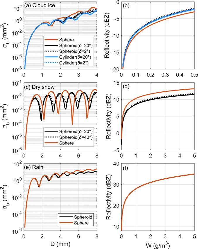
Figure 10 shows a radar reflectivity comparison between reflectivity peak in the vertical profile from the conventional
the simulation results and CloudSat CPR observation data. simulation was 13 dBZ at approximately 2.6 km with a bright
The cross sections in Fig. 10a and b show simulation re- band width of approximately 1.4 km. In summary, the melt-
sults, where Fig. 10a corresponds to the improved micro- ing model can accurately capture the stratiform cloud precip-
physical parameter settings shown in Fig. 9h, and Fig. 10b itation characteristics.
corresponds to the conventional setting. Figure 10c shows
the observation results from the CloudSat CPR. The lines 4.2 Convective case
in Fig. 10d show the average vertical profiles of the reflec-
tivity factor in Fig. 10a–c. The echo structure and echo in- 4.2.1 WRF scenario simulation
tensity of the simulation results with the improved setting
showed a good agreement with the CloudSat observations. This case was a severe convective weather process that oc-
The trends in the two profiles were basically identical; the curred in the lower Yangtze–Huaihe River on 23 June 2016,
relative error (|Zsim − Zobs |/Zobs , where Zsim represents the in which strong winds and heavy rainfall occurred in the
simulated reflectivity and Zobs represents the observations; cities of Yancheng and Lianyungang, Jiangsu Province. The
simulation area covered 32–36◦ N and 116–120.5◦ E. Triple
https://doi.org/10.5194/amt-16-1723-2023 Atmos. Meas. Tech., 16, 1723–1744, 20231736 L. Kou et al.: Simulation and sensitivity analysis of spaceborne radar cloud and precipitation
than 100 mm. The rainfall area in the simulation is similar to
that from rain gauge data, and three heavy rainfall centers can
be seen in the model result. The maximum rainfall from rain
gauge data is approximately 120 mm, and the maximum from
the WRF is approximately 126 mm. The amount, scope, and
distribution of rainfall from the WRF simulation are gener-
ally consistent with the rain gauge data. The main difference
is in the strong rainfall location and extreme value. Consid-
ering the model limitations, the comparison results show that
the model captured the convective precipitation process.
4.2.2 Experiment design
CloudSat observed this convective process at 04:30 UTC on
23 June 2016, covering the cloud region from 32.43◦ N,
119.13◦ E to 36.11◦ N, 118.10◦ E. For comparison with the
CloudSat data, the vertical cross section of the hydrometeor
matching the CloudSat observation was selected for sim-
Figure 10. Radar reflectivity comparison between the simulation ulation. Figure 12a–f show the latitude–height cross sec-
results and CloudSat CPR observation data for the stratiform cloud tion of the hydrometeor for the convective case simulated
precipitation case. (a) Cross section of the simulation result with by the WRF for the total hydrometeors, cloud water, cloud
the improved setting, (b) cross section of the simulation result with ice, snow, graupel, and rain. The ice water content of the
the conventional setting, and (c) cross section of the CloudSat CPR convective case was large, and the vertical extent of cloud
observation data. (d) Vertical profiles of the average reflectivity in ice, snow, and graupel particles was widely distributed with
(a)–(c), where the red line represents the simulation result with the high contents. Snow existed from 4 to 14 km, with a water
improved setting, the blue line represents the simulation results with content reaching approximately 1.5 g m−3 . Graupel particles
the conventional setting, and the black line represents the results of mainly ranged from 4–8 km, with a maximum water content
the CPR observation. Owing to the melting modeling in the im-
of 1.2 g m−3 . Rain was mainly distributed between 34 and
proved simulation, the echo structure and intensity were consistent
with the CPR observation results.
36◦ N, and the water content of the rain near 34.5 and 34.8◦ N
reached 5 g m−3 .
In the convective case, snow and graupel were abundant.
Unlike stratiform clouds, a large percentage of heavily ag-
nested grids were adopted, with horizontal resolutions of gregated and/or rimed snow commonly exists in convective
22.5, 7.5, and 1.5 km. More details about the WRF model clouds (Yin et al., 2017); therefore, rimed particles were as-
setup for the convective case can be found in Appendix A. sumed for convective cloud modeling. Considering the ef-
For validating the model result, the ERA5 data, ground fect of riming, a varying mass–power relationship was as-
radar reflectivity, and rain gauge data were used. Figure 11a– sumed in the simulation with the improved setting. As the
f compare the fraction of cloud cover, reflectivity, and rainfall prefactor a in the mass–power relations increases with the
from the WRF model with the observation data. Figure 11a riming degree (Mason et al., 2018; Moisseev et al., 2017;
shows the fraction of cloud cover from the WRF model at Ryzhkov and Zrnic, 2019), an adjustment factor f was con-
the d02 domain. The cloud area and coverage are consistent sidered in the simulation process, i.e., a = au f , where au is
with the ERA5 data shown in Fig. 11b. Figure 11c and d the density prefactor for unrimed snow. f is obtained from
compare the reflectivity from the WRF simulation over the f = 1/(1 − FR), where FR is the ratio of the rime mass to
d03 domain at 04:00 UTC on 23 June and ground radar at the snowflake mass. According to Moisseev et al. (2017),
Lianyungang at 04:02 UTC on 23 June 2016. From radar ob- FR can be expressed as a function of the effective liquid wa-
servation, we can see that the strong echo area is relatively ter path (ELWP), ELWP ≈ 4αu /π · FR/(1 − FR), given that
scattered, generally trending from northwest to southeast, the rime mass is determined by the mass of swept super-
and the maximum reflectivity is about 55 dBZ. In the sim- cooled liquid droplets. Considering the connection between
ulation, the strong radar echo is mainly distributed along the ELWP and liquid water path (LWP) (according to Moisseev
northwest–southeast; the radar echo structure and echo in- et al., 2017, ELWP is approximately half of LWP), we as-
tensity are close to the radar observation. Figure 11e and f sumed that the adjustment factor f increased linearly with
show the 6 h accumulated rainfall from 00:00 to 06:00 UTC LWP, and the relation between f and LWP was derived to
on 23 June from the WRF model and rain gauge data, respec- be f ≈ 0.5π LWP/αu + 1. The assumption ignores possible
tively. The rainfall covers most areas in the north of Jiangsu changes in particle mass linked to the presence of differ-
Province, and there are two heavy rainfall centers of more ent crystal habits, and the exponent b in the mass–size re-
Atmos. Meas. Tech., 16, 1723–1744, 2023 https://doi.org/10.5194/amt-16-1723-2023You can also read