Short-range ocean forecast error characteristics in high resolution assimilative systems - Met Office

Page created by Ashley Page

Current Events

English

Like
Share
Embed
Fullscreen
Slides
Download HTML
Download PDF
Abuse

←

→

Page content transcription

If your browser does not render page correctly, please read the page content below

Short-range ocean forecast error characteristics in high resolution assimilative systems - Met Office

Short-range ocean
forecast error
characteristics in high
resolution assimilative
systems
March 25, 2021

Technical Report No: 645

Davi M. Carneiro 1 , Robert King 1 , Matthew Martin 1 and
Ana Aguiar 1
1
Met Office, Exeter, UK

 www.metoffice.gov.uk © Crown Copyright 2021, Met Office

OFFICIAL-SENSITIVE

Executive summary
This work assesses short-range forecast error characteristics of high-
resolution assimilative ocean forecasting systems based on NEMO. The resolution of the
models used ranges from 1/4° to 1/12° globally and down to 1.5 km in the North-West
European Shelf-Seas region. The regional model includes processes not represented in the
global models such as tides and a better representation of the complex bathymetry in the
region. A common set of high-resolution satellite data (as well as in situ observations) are
assimilated into each of these configurations which are all used in CMEMS forecasting
systems. A common two-year period is used for all the integrations with a common set of
surface atmospheric forcing so that the forecast error characteristics can be estimated in a
consistent way. Additionally, the 1.5 km model is forced by two different sets of atmospheric
fields to understand their impact on the magnitude and scales of the forecast errors.
Two methods are used to estimate the forecast error characteristics for sea surface
temperature (SST). The first is based on the observation-forecast differences (called the
innovations) and the second is based on differences in two forecasts of different lengths, both
valid at the same time. Both sets of information about the forecast errors are used to
extract seasonal information about the forecast error covariances and the results are
summarised by estimating length-scales and variances associated with two components
of the SST errors. The results show a clear seasonality in the SST forecast errors in both
global configurations, with increased errors in the summer hemisphere. Although both global
configurations have similar seasonal variations, the system at 1/12° resolution gives
larger SST small-scale errors than the one at 1/4° resolution. This increase of the small-scale
errors in the 1/12° global configuration is mostly associated with the increase of the error
covariances within 25 km of separation distance, consistently seen in the boundary
currents. Further improvements should be made to the assimilation in the 1/12° global
system to properly constrain fine-scale structures, which are not present at a resolution of
1/4°. The impact of the surface forcing on the representation of the forecast errors is unclear
with different results given by the error covariance methods, and further investigation is
necessary to understand these differences. However, in contrast to the 1/12° global system,
the benefits of increasing the model resolution to 1.5 km in the North-West European shelf is
clearly seen, with an overall reduction of the small-scale SST forecast errors and their
associated length-scales in the shelf seas and deep part of the domain. Therefore,
the positive impact of 1.5 km systems on properly reproducing fine-
scale SST features reinforces the large potential for future higher-resolution global
models that are currently being developed by operational centres. In addition to the impact of
the resolution on the forecast errors, the error covariance estimates produced here will also
be used to update the model background error parameters in the data assimilation
system, which is expected to reduce the forecast errors of these model configurations in the
future.

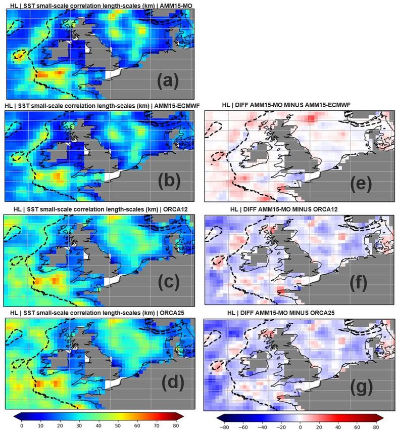
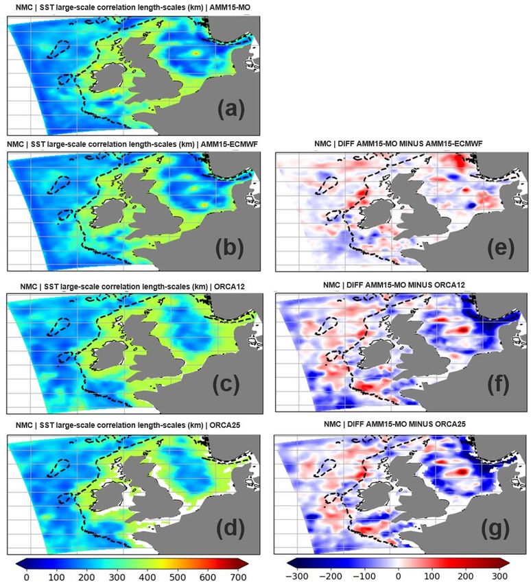
OFFICIAL-SENSITIVE

Contents

1. Introduction .................................................................................................................... 4
2. Model and data assimilation system description............................................................. 6
 2.1 Global models ......................................................................................................... 8
 2.2 Shelf-seas model .................................................................................................... 8
 2.3 Data assimilation .................................................................................................. 10
 2.4 Description of assimilated observations ................................................................ 11
3. Methods for estimating error covariances..................................................................... 12
 3.1 Innovations-based method .................................................................................... 14
 3.2 Forecasts of different lengths ................................................................................ 16
4. Results ......................................................................................................................... 17
 4.1 Global error covariances ....................................................................................... 17
 4.1.1 Comparison of HL estimates between VIIRS and drifter innovations .............. 17
 4.1.2 Small-scale forecast error variances .............................................................. 19
 4.1.3 Large-scale forecast error variances .............................................................. 22
 4.1.4 Forecast error length-scales .......................................................................... 24
 4.1.5 Forecast error covariances at short separation distances .............................. 28
 4.2 North-west European shelf-seas error covariances ............................................... 31
 4.2.1 Small-scale forecast error variances .............................................................. 31
 4.2.2 Large-scale forecast error variances .............................................................. 33
 4.2.3 Small-scale forecast error length-scales ........................................................ 33
 4.2.4 Large-scale forecast error length-scales ........................................................ 34
 4.2.5 Forecast error covariances at short separation distances .............................. 34
5. Discussion and conclusions ......................................................................................... 39
References ......................................................................................................................... 43

© Crown copyright 2021, Met Office Page 3 of 48

OFFICIAL-SENSITIVE

1. Introduction

Short-range ocean forecasts are produced operationally at many centres around the world
with the forecasts used for various applications including ship routing, oil spill modelling,
search and rescue, and Naval operations (Davidson et al., 2019). The ocean analyses from
such systems are also used to initialise coupled ocean/atmosphere forecasts from short-range
out to seasonal and decadal timescales (Guiavarc’h et al., 2019; Penny et al., 2019). A good
estimate of the current state of the ocean is required to produce these forecasts, and this is
done using data assimilation methods which combine the available in situ and satellite
observations with the ocean model (see Moore et al., 2019 for a recent review).
For short-range ocean and coupled prediction in particular, many applications need high
resolution information about the ocean. For global scales, eddy resolving models are now run
at many operational centres with Mercator Ocean and the Met Office now running 1/12° global
systems operationally for instance (Lellouche et al., 2018; Aguiar et al., 2021) and CMCC
running a 1/16° global system (Iovino et al., 2016). Higher resolution global systems are being
run elsewhere: for instance, the US Navy currently runs a 1/25° global version of HYCOM to
produce operational forecasts (Barton et al., 2020); Mercator Ocean is currently developing a
1/32° global system for future implementation.
Regional forecasting systems are often run at even higher resolution than the above global
systems (De Mey-Frémaux et al., 2019). This extra resolution is often needed to represent
processes which are important for regional and coastal applications which attempt to represent
the ocean state in regions including sharp bathymetric features, complex coastlines and in
shallower waters where tides are important. The Met Office for instance currently runs a 1.5
km resolution version of NEMO to produce operational forecasts for the North West European
Shelf Seas (NWS) as part of the Copernicus Marine Environment Monitoring Service
(CMEMS; Tonani et al., 2019).
The aim of this work is to improve our understanding of the error characteristics of high-
resolution global and shelf-seas forecasting systems. This includes understanding not only
the magnitude (variance) of the forecast errors, but also their spatial characteristics (their
covariances). Such an understanding is useful for several reasons. Users of the forecast data
often want to know how accurate the data are, so the forecast error variance information is
useful for them. When designing observing systems for assimilation and forecasting
applications, information about the spatial scales of the errors can help to determine the
optimal sampling strategy in different regions. Data assimilation systems also need
information about the forecast error covariances to make best use of the observations.
Information about the forecast errors can also help to identify areas where the forecasting
systems can be improved through model and data assimilation development and can be used
to understand whether increases in model resolution lead to better forecasts.
Estimation of forecast errors is a large topic which has been addressed by many authors both
for verification/validation purposes and for data assimilation applications. The fundamental
issue with this subject is that there is no spatially and temporally complete estimate of the
“true” ocean with which to compare the forecasts. Observations are the only source of direct

OFFICIAL-SENSITIVE

information about the ocean, but they are spatially and temporally incomplete and suffer from
various types of error. Proxies for the true error can be obtained by comparing model forecasts
of differing lengths, valid at the same time. This has the advantage of providing information
everywhere at the resolution of the model grid but can suffer from issues when the
observations being assimilated are sparse compared to the scales of the errors and/or when
there is model bias. Ensembles can also be used to estimate uncertainties in the forecast, but
the results depend on the ensemble generation strategies adequately representing the various
sources of uncertainties in the forecast, and there being a large enough ensemble to avoid
sampling issues, which is very expensive to do when dealing with high resolution models. A
comprehensive review of these various methods for estimating forecast error covariances has
been written by Bannister et al. (2008) with a focus on atmospheric data assimilation. Another
approach to tune the error covariances in a data assimilation system is the one originally
proposed by Desroziers et al. (2005) which uses differences between observations, analysis
and forecast solutions at the observation locations. This was shown by Mattern et al. (2018)
to improve the quality of a regional ocean data assimilation system, but their approach scales
an existing forecast error field for each variable, assuming that its underlying spatial structure
is correct. We do not apply the Desroziers method here since we aim to provide a good
estimate of the underlying spatial structure of the forecast error, and compare those structures
between different assimilative systems. Further work could include its application to further
tune the error covariances estimated in this work.
Roberts-Jones et al. (2016) used observation-forecast differences to estimate the error
covariances of sea surface temperature (SST) in the Operational sea Surface Temperature
and sea Ice Analysis (OSTIA) system. The work described here follows on from that work by
applying similar methods to understand the forecast errors in high resolution global and
regional forecasting systems, as well as using the forecast-difference approach mentioned
above. The observation operator code in NEMO (which interpolates model information to the
observation locations at the nearest model time-step) is used to generate the information for
the observation-based method. Python code has been developed to perform these
calculations and has been made freely available via a Github repository.
Outputs from three different configurations of the NEMO model (Madec, 2016), all employed
for operational forecasting in the Met Office, are used: i) a global 1/4° resolution system, ii) a
1/12° resolution global system and (iii) two versions of a 1.5 km resolution system for the NWS
region, with different sets of atmospheric forcing. A common experiment framework is used to
produce analysis and forecast data over two years for these configurations: the same version
of NEMO (version 3.6; Madec, 2016) is used for all systems, the observations input to the data
assimilation are the same, and the data assimilation systems use a common 3DVar-FGAT
(First Guess at Appropriate Time) scheme based on the NEMOVAR code (Mogensen et al.,
2012). High resolution observational datasets need to be assimilated for the forecast error
covariance estimation methods to work well, and we assimilate swath SST data from many
satellites into these systems along-side in situ SST data, observations from satellite altimeters,
in situ profiles of temperature and salinity, and satellite sea-ice concentration data (in the
global systems).
More detail on the model and data assimilation systems as well as the observations

OFFICIAL-SENSITIVE

assimilated is given in section 2. The methods used to estimate the forecast error
characteristics are described in section 3. The estimated error covariances are presented in
section 4, including: a comparison of the results from the different methods; an assessment of
the impact of the model resolution on the error covariances and their spatial scales, both
globally and for the NWS region; and an assessment of the impact of the atmospheric forcing.
A discussion of the main results and the conclusions are presented in section 5.

2. Model and data assimilation system description

The experiments described in this report use different configurations of the same underlying
ocean analysis and forecasting system: the Met Office Forecasting Ocean Assimilation Model
(FOAM) system. For the global experiments, we use the 1/12° ORCA12 and 1/4° ORCA025
configurations of FOAM, while for the higher resolution regional experiments, we use the 1.5
km resolution AMM15. All these systems are run operationally to produce analyses and
forecasts, and we use the most recent version of the systems. All the FOAM configurations
use the NEMO ocean model and the NEMOVAR assimilation scheme with a 24-hour
assimilation window. Each assimilates broadly the same observations, but with configuration-
specific observation averaging and quality control (as detailed below). On each day a two-day
forecast was run to allow the calculation of short-term forecast errors.
To illustrate the differences in characteristics of the three different configurations used here,
Fig. 1 shows the daily mean surface currents in the region of the AMM15 configuration.
Although the main dynamical features are in similar locations, there is a clear change in
character between the ORCA025 and ORCA12 configurations, with ORCA12 having sharper
features with stronger currents. Comparing ORCA12 with AMM15, the higher resolution
system can represent much smaller scales in the deeper part of the region and exhibits
different characteristics to the flow in the shallower waters.
All simulations were initialised in June 2016 from a spun-up state from previous reanalysis
runs with an older version of the system and different sets of observations, and they were run
for a period of 6 months prior to being used in the error covariance calculations from 1 st
January 2017. The global simulations were then run to the end of 2018, while the AMM15
simulations were run to June 2018. After discarding the 6-month spin-up period, this provided
a 2-year ORCA12, a 2-year ORCA025, and 18-month AMM15 simulations. A summary of the
experiments used in the forecast error calculations is given in Table 1.

OFFICIAL-SENSITIVE

 Figure 1: Daily mean surface current speed in the AMM15 domain from the three FOAM configurations for 1 st
 January 2018.

Configuration Model Grid resolution of Surface forcing and Period
 model/assimilation resolution

ORCA025 NEMO/CICE 1/4° (1/4°) MetUM (17 km -> 10 km) 1/1/2017-31/12/2018

ORCA12 NEMO/CICE 1/12° (1/4°) MetUM (17 km -> 10 km) 1/1/2017-31/12/2018

AMM15-MO NEMO/WWIII 1.5 km (1.5 km) MetUM (17 km -> 10 km) 1/1/2017-30/6/2018

AMM15-ECMWF NEMO/WWIII 1.5 km (1.5 km) ECMWF IFS (14 km) 1/1/2017-30/6/2018

 Table 1. Summary of the experiments used as input to the error covariance calculations.

 © Crown copyright 2021, Met Office Page 7 of 48

OFFICIAL-SENSITIVE

2.1 Global models

The FOAM-ORCA12 and FOAM-ORCA025 configurations use the NEMO ocean model
version 3.6 (Madec, 2016) coupled to the Los Alamos sea ice model (CICE; Hunke et al.,
2010) in the GO6 configuration described by Storkey et al. (2018) and the GSI8 configuration
described by Ridley et al. (2018). Both configurations have a non-linear-free surface and 75
vertical levels, with 1 m vertical resolution at the surface and decreasing resolution with
increasing depth. The three-fold increase in horizontal resolution from ORCA025 to ORCA12
encompasses the transition from eddy-permitting to eddy-resolving scales at most latitudes
(see Fig. 2). In both configurations, the ocean is forced at the surface using hourly momentum
and 3-hourly freshwater and heat fluxes from the operational Met Office Unified Model
(MetUM) global Numerical Weather Prediction (NWP) system. The resolution of the
atmospheric forcing is about 17 km for the period up to mid-July 2017, and then increases to
about 10 km after that. Both these configurations are currently run operationally at the Met
Office. The ORCA025 configuration is used as part of a coupled forecasting system
(Guiavarc’h et al., 2019) which provides ocean forecasts to CMEMS, while the ORCA12
configuration is producing operational forecasts for the UK Royal Navy (Aguiar et al., 2021).
A similar ORCA12 configuration is used to produce global ocean forecasts for CMEMS by
Mercator Ocean.

Figure 2: Rossby radius (km) (left) and model grid resolution (km) as a function of latitude (right) for ORCA025 and
ORCA12.

2.2 Shelf-seas model

The FOAM-AMM15 configuration employs the same system as used in the operational Met
Office North-West European Shelf ocean forecasting system (Tonani et al., 2019) which
delivers forecast products to CMEMS. This system couples the NEMO ocean model, also at
version 3.6, with the WAVEWATCH III spectral wave model (Saulter et al. 2017; Lewis et al.
2019). The domain (shown in Fig. 2) extends from approximately 45°N, 20°W to 63°N, 11°E
on a rotated pole grid, covering the north-west European Shelf and part of the north-east
Atlantic Ocean. This domain has a complex bathymetry, containing regions of shallow water,

OFFICIAL-SENSITIVE

a continental shelf, and regions of deep ocean (i.e. depths greater than 5000 m). The resulting
dynamics produce mesoscale eddies along with seasonally stratified and well-mixed regions
with marked boundaries. The large changes in bathymetry mean that there is a wide range of
scales associated with the first baroclinic Rossby radius (also shown in Fig. 3). In the shallow
waters of the shelf the Rossby radius is smaller than 5 km, while in the deeper ocean it is
closer to 25 km.

Figure 3: Rossby radius (km) (top) and Bathymetry (m) (bottom) for AMM15.

The ocean model component uses the eddy-resolving 1.5 km Atlantic Margin Model
configuration (AMM15, Graham et al., 2018) of NEMO version 3.6 (Madec 2016). The model
employs a non-linear free surface, 51 vertical terrain-following levels and includes 11 tidal
constituents, specified on the open boundary via the Flather radiation condition (Flather et al.,
1981). The AMM15 is nested within the Met Office 1/12° North Atlantic model (NATL12;
Storkey et al. 2010; Blockley et al. 2014) which provides the lateral boundary conditions,
except for the Baltic boundary which is taken from the CMEMS Baltic Sea model (Berg et al.,
2012). The ocean and wave components are coupled hourly using the OASIS3-MCT coupler
(Craig et al., 2017).
The operational version of this system is forced at the surface using ~14 km resolution, 3-
hourly wind and atmospheric pressure fields, radiative and E-P (evaporation-minus-
precipitation) fluxes from the ECMWF operational Integrated Forecasting System (IFS).
However, as detailed above, the FOAM-ORCA12 system uses surface forcing from the
operational Met Office global atmospheric model (~10 km horizontal resolution, hourly wind

© Crown copyright 2021, Met Office Page 9 of 48

OFFICIAL-SENSITIVE

and pressure, and 3-hourly radiative and E-P fluxes). Therefore, to investigate the impact of
the different forcing, we have run two AMM15 simulations: one forced by the ECMWF IFS
fluxes, and the other forced by the Met Office UM fluxes. In each case, the wave and ocean
models are forced by the same wind fields, and the wave model uses the surface currents
computed by the ocean model.

2.3 Data assimilation

The NEMOVAR data assimilation scheme is used in all configurations of the operational Met
Office ocean analysis and forecasting systems. This is a multi-variate, multi-lengthscale
assimilation scheme developed collaboratively by the Met Office, Centre Europeen de
Recherche et de Formation Avancee en Calcul Scientifique (CERFACS), the European Centre
for Medium Range Weather Forecasts (ECMWF), and Institut National de Recherche en
Informatique et en Automatique (INRIA) (Mogensen et al. 2009; Mogensen et al. 2012; Waters
et al. 2015). The implementation in the global configurations is based on that used in the
ORCA025 system as described by Waters et al. (2015) and Mirouze et al. (2016). In the
AMM15 system the implementation is as described for a lower resolution regional AMM7
system by King et al. (2018), with modifications for application to AMM15 as described by
Tonani et al. (2019).
An assimilation window of 24 hours is used to assimilate observations including satellite and
in situ SST, satellite altimeter observations of the sea level anomaly (SLA), and in situ
temperature and salinity profiles from a variety of platforms. The systems include a variational
bias correction scheme for SST and SLA observations (While and Martin, 2019; Lea et al.,
2008) and the assimilation increments are added incrementally over 24 hours through an
incremental analysis update (Bloom et al. 1996). In the ORCA025 and AMM15 configurations,
the assimilation is carried out on the same grid as the ocean model. However, in the current
implementation of ORCA12, the assimilation takes place on the ORCA025 grid and
increments are interpolated to ORCA12 ahead of the incremental analysis update.
NEMOVAR uses linearised balance relationships to account for correlations between ocean
variables as defined by Weaver et al. (2005). The temperature-salinity balance operator is a
linearised version of the water-mass property conservation scheme of Troccoli & Haines
(1999). The sea surface height (SSH) balance operator is a linearised version of the Cooper
& Haines (1996) scheme in which SSH changes are associated with the lifting and lowering
of the entire water column. The velocity balance operators are based on the geostrophic
relation, density balance is the linearised equation of state, and the pressure balance is the
vertically integrated hydrostatic equation.
The background error covariance is approximated using an estimate of the model variable
variances and with background‐error correlations modelled using a diffusion equation
(Mirouze & Weaver, 2010). Various options exist in NEMOVAR for how to apply the diffusion
equation to model the spatial correlations. It can be solved explicitly or implicitly, and it can be
used to represent isotropic or anisotropic correlation structures (Weaver and Mirouze, 2013).
Various functions belonging to the class of Matérn functions (which contains the Gaussian

OFFICIAL-SENSITIVE

function) can be represented efficiently using the implicit solution to the diffusion equation. In
the FOAM system we use the implicit solution to the diffusion equation to model a combination
of two isotropic Gaussian functions. This uses a combination of a short and a long length-
scale to account for errors in both internal ocean processes and larger-scale errors from the
atmospheric forcing (Mirouze et al., 2016). In each configuration, the short horizontal
correlation length‐scales are prescribed through the first baroclinic Rossby radius. In each
case, the minimum length-scale is capped to avoid numerical issues (25 km for ORCA025,
and 4.5 km for AMM15). Furthermore, in the global configurations the maximum short length-
scale is capped at 150 km near the equator. The long background error correlation length-
scale is set to 400 km in the global configurations and to 100 km in the AMM15.
The current observation and background error variances in NEMOVAR are specified using a
combination of statistical estimates and parameterisations. The surface temperature, salinity,
and unbalanced SSH error variances are specified based on spatially and seasonally varying
estimates calculated from earlier model runs with ORCA025 and AMM7. The sub-surface
temperature/salinity background errors are parameterised as follows. The surface value is set
by the statistical estimate mentioned above and a minimum value at each model level is
defined by a tapered function of the surface value. To introduce some flow dependence, the
vertical temperature/salinity gradient is then calculated from the background field at all grid-
points. Below the base of the mixed layer, the background error standard deviation is defined
as the larger of the tapered surface value or a parameterisation of the temperature/salinity
gradient (e.g. δz*(dT/dz), where δz=20 m, as described by Waters et al. 2015). This results in
the largest errors occurring at the thermocline/halocline, allowing the observations to have
greater weight to shift the depth of the thermocline/halocline.
In this work we are producing new estimates of the forecast error covariances based on the
methods described in section 3. This will lead to new spatially and seasonally varying
estimates of the error covariances which can then be used to improve the various
specifications in the data assimilation described above. The work is therefore expected to
feedback into improvements in the data assimilation which should lead to reduced forecast
errors in these configurations in the future.

2.4 Description of assimilated observations

Each of the three configurations assimilates broadly the same set of observations: in situ and
satellite SST observations, satellite altimeter observations of the sea level anomaly, and in
situ temperature and salinity profiles from several platforms. The global configurations also
assimilate satellite observations of the sea-ice concentration (the regional AMM15 has no sea-
ice component).
The in-situ SST observations assimilated include observations from ships, surface drifters,
and moorings. We also assimilate L2p/L3c satellite swath observations of SST from
NOAA/AVHRR, MetOp/AVHRR, MSG/SEVIRI, Sentinal-3/SLSTR, and Suomi-NPP/VIIRS. All
these data were distributed in Near-Real Time (NRT) by the Group for High Resolution SST
(GHRSST). In the global configurations, these data were used with a spatial median averaging

OFFICIAL-SENSITIVE

over a 13 km radius for each satellite type, while in the higher resolution AMM15 no
observation averaging was done.
A background check was performed for the SST observations where each observation was
compared to the model background at the nearest time-step and interpolated to the
observation location. Using the specified observations and background errors, any
observation with a probability of gross error exceeding 50% was rejected. Biases in the
satellite observations are accounted for using an on‐line bias correction scheme described by
While and Martin (2017) which uses the in situ drifters and a sub-set of the VIIRS data (night-
time data near the centre of the swath) as anchor observations.
Along‐track satellite altimeter SLA data from CMEMS are assimilated with an on‐line bias
correction scheme to account for errors in the mean dynamic topography (MDT; see Lea et
al., 2008) and residual errors due to atmospheric effects. While the global configurations
assimilate the standard SLA data which removes the effects of tides and the ocean barotropic
response to the wind forcing, the AMM15 uses supplied corrections to ensure the assimilated
SLA includes the effects of wind and pressure as these physical processes are included in the
regional model. Although the tidal contribution of the observed SLA is also provided, this is
not used as the tides are removed from the AMM15 model counterpart before calculating the
SLA innovation.
Quality-controlled in situ profile observations of temperature and salinity were taken from the
EN4 dataset (Good et al., 2013). This dataset includes temperature and salinity profiles from
Argo floats, moored buoy arrays, XBTs, CTDs, gliders, and marine mammals.
Sea‐ice concentration observations from Special Sensor Microwave Imager/Sounder
(SSMI/S) satellite instruments, processed by the European Organisation for the Exploitation
of Meteorological Satellites (EUMETSAT) Ocean and Sea‐Ice Satellite Application Facility
(OSI‐SAF) are assimilated in the global ORCA025 and ORCA12 configurations.

3. Methods for estimating error covariances
We use two methods for estimating the forecast error covariances. The first method is based
on observation-minus-forecast data, where the model data are interpolated to the observation
location at the nearest model time-step during a one-day forecast of NEMO. It was originally
proposed by Hollingsworth and Lonnberg (1986) so we refer to it as the HL method here. More
recently, Roberts-Jones et al. (2016) used that method to estimate error covariances for the
OSTIA system and we follow their approach. The HL method relies on a dense sampling by
the observations which is a challenge for the ocean since itis relatively sparsely observed
compared to the atmosphere. The aim of this work is to investigate forecast errors for high
resolution systems, so we chose to focus on sea surface temperature (SST) which is the
variable with the densest observing network. One drawback of the HL method is that it
assumes that any spatial covariances in the observation-model differences are due to forecast
errors, and that the observation errors are uncorrelated spatially, so we have to be careful
about which SST satellite data types we use. The advantage of the HL method is that it

OFFICIAL-SENSITIVE

provides direct estimates of the forecast errors without needing to make assumptions about
the behaviour of the model forecast errors.
To complement the HL method with another method that can provide information about the
forecast errors at higher spatial resolution, we use the NMC method, originally proposed by
Parish and Derber (1992). This method uses forecasts of different lengths valid at the same
time as a proxy for the forecast error. This has the advantage that we get information about
the forecast errors at the resolution of the model grid, but it does make assumptions about the
behaviour of the model in order for this to be a good proxy for the real error. A more detailed
description about the HL and NMC methods and how we apply them are given in the next two
sub-sections.
As discussed in the introduction, other methods are available for estimating forecast error
covariances, including ensemble-based methods. We discount this type of method for this
work since it is too computationally expensive to run a reasonable size ensemble of the high-
resolution assimilative forecasting systems we are interested in. For example, an ensemble
system for ORCA025 is currently being developed at the Met Office, but applying the same
strategy is still too computationally expensive for the high-resolution model configurations,
such as ORCA12 and AMM15. Error covariances for ORCA12 could still be produced based
on the ORCA025 ensemble, however they would not be fully optimal as the ORCA025
ensemble is not expected to represent the same fine-scale structures generated by the
ORCA12 system.
The HL method allows us to produce estimates of the forecast errors on a pre-defined
(determined by having adequate observation sampling) regular grid, while the NMC estimates
are made on the model grid. We calculate the covariance information on each day and
accumulate the information over seasons (with 2-years’ worth of data as described in the
previous section). Both methods allow us to produce “local” statistics of the covariances of the
forecast error either with observation locations near a particular point (for the HL method) or
model grid-points near a particular point (for the NMC method). We cannot afford
computationally to produce “global” error covariance estimates for every point with all other
points around the globe. We restrict the distances over which the error covariances are
calculated to be within 500-1000 km depending on the configuration and assume that the error
covariances at longer distances are small. Even with this simplification, the error covariance
calculations produce very large volumes of data from which we need to distil information about
the magnitude and spatial characteristics of the errors.
To summarise the information about the error covariances from both methods, we assume a
functional form of the error covariances, and produce estimates of the function’s parameters
by fitting it to the covariance data at each grid point. The function we use is a combination of
two Gaussian functions, each with their own amplitude and their own length-scale:
2 /(2 2 ) 2 /(2 2 )
( ) = 1 − 1 + 2 − 2 . ( 1)

Here and are the forecast error variance and the length-scale for component , and is
the separation distance between two points. At zero separation distance, the forecast error
variance is the sum of the variance associated with each component. It has been shown in

OFFICIAL-SENSITIVE

previous studies (e.g. Martin et al., 2007) that the errors in ocean forecasts often have two
components to their errors and that using a combination produces a much better fit to the
covariance data than a single function. Physically we expect there to be errors on scales
associated with internal ocean model dynamics which may occur at the mesoscale, and errors
associated with atmospheric forcing which may have scales similar to those of atmospheric
phenomena (e.g. synoptic systems). These two length-scales are deduced iteratively from the
fit with Eq. 1, and the initial guesses for the small and large length-scales are defined as 40
and 400 km, respectively. There is a question as to whether more than two length-scales
should be used for very high-resolution systems which may have a third error component
associated with sub-mesoscale processes.
A summary of the methods used is:
1. On each day, generate information about the forecast errors using either the HL or
NMC methods described in the next sub-sections. This information is accumulated on
a predefined grid (regular grid for the HL method and the model grid for the NMC
method). For the HL method a pre-defined set of separation bins is used to accumulate
the covariance statistics. For the NMC method the model grid-points surrounding the
current grid point are used with the number of grid-points described in the next sub-
sections.
2. Accumulate the daily forecast error covariance information over each month, then
combine the monthly statistical information into seasons and into files for the entire
experiments.
3. Fit the function defined in equation (1) to the covariance statistics produced at each
grid point.
Python code has been developed to do the above calculations and has been made publicly
available from a Github repository (https://github.com/MetOffice/ocean_error_covs). This
currently includes only the code to perform the HL calculations, but will be updated soon to
include the NMC code.

3.1 Innovations-based method

As described above, the HL method uses information at observation locations to determine
the error covariances. The differences between the observations, , and the model forecast,
, interpolated to the observation locations using the observation operator, ℎ, are known as
the innovations and are denoted . They are comprised of the observation errors, , and the
model forecast errors, :

= − ℎ( ) = ( − ℎ( )) − (ℎ( ) − ℎ( )) = − ,

where is the true ocean state represented on the model grid. Here we use systems with a
one-day assimilation cycle and therefore use the model values during a one-day forecast to
form the innovations. Pairs of innovations at locations and are used to estimate the error
covariances. Assuming that the observation errors and forecast errors are not cross-

OFFICIAL-SENSITIVE

correlated, and that spatial correlations in the observation errors are much smaller-scale than
in the forecast errors, we can write the following:
 
 < > = < ( − )( − ) >=< − − + >
 
 < ( )2 > +< ( )2 > ℎ = 
 = { 
 < > ℎ ≠ 

where the brackets denotes the expectation operator. So, under the above assumptions,
the variance of the innovations is comprised of the sum of the observation error variance and
the forecast error variance. The covariances of the innovations, for separation distances
between locations and greater than zero, provides information about the forecast error
covariances. In the HL method, parameters of a pre-defined function (here defined in equation
(1)) are estimated by fitting the function to the forecast error covariance data with separation
distances greater than zero. The forecast errors can then be extrapolated to the zero-
separation point using that function to estimate the forecast error variance. The observation
error variances can also be determined by subtracting the forecast error variance from the
total variance of the innovations, though we focus here only on the forecast errors.
There are two aspects to the spatial resolution of the resulting error covariance estimates.
One is the grid on which the estimates are accumulated. Here we use a 1° grid which was
determined to allow enough observations to avoid issues with sampling noise, yet still allow
us to estimate useful spatial variations in the covariance parameters. The second aspect is
the resolution on which to accumulate the spatial covariance statistics, i.e. the separation
distances. Again, we tested various options for these, and ended up using 18 bins with the
distances for the global estimates of 10, 15, 20, 50, 100, 150, 200, 250, 300, 350, 400, 450,
500, 600, 700, 800, 900 and 1000 km. For the estimates in the NWS region, 24 bins were
used with the following distances of 10, 15, 20, 30, 50, 75, 100, 125, 150, 175, 200, 225, 250,
275, 300, 350, 400, 450, 500, 550, 600, 700, 800 and 900 km. It would be possible to estimate
anisotropic aspects of the error covariances by looking in different directions when
accumulating the error covariance statistics, but we do not do that here. Isotropic error
covariances may be questioned in specific regions of the ocean (e.g. in the tropics or along
land boundaries), but chi-squared tests were calculated to evaluate the goodness of the
function fitting for each point of the grid. Although chi-squared values are slightly larger along
the land boundaries, their values are very close to zero almost everywhere (not shown),
indicating that the fitting of isotropic error covariances is well suited for the purposes of this
report.
In terms of the observation types which we used for these estimates, there are several SST
satellite instruments which we can choose from. We decided to use the VIIRS data for these
calculations since they are very numerous, and have been shown to be unbiased (they are
used as reference data in the variational bias correction scheme carried out as part of the data
assimilation process). The HL method assumes that correlations in the observation errors are
much smaller-scale than in the forecast errors. For high-resolution satellite data such as
VIIRS, this condition is more likely to be achieved by thinning the observations (i.e. using a
subset of available observations) or by calculating super-observations (i.e. averaging subsets

© Crown copyright 2021, Met Office Page 15 of 48

OFFICIAL-SENSITIVE

of available observations). As mentioned in section 2.4, the latter is applied to VIIRS data in
the global configurations, but in higher resolution AMM15 no observation averaging is carried
out. It is worth noting that only assimilated VIIRS observations are considered for the HL error
covariance calculation. In order to understand whether the assumption of small spatial
correlations in the observation errors is valid, HL error covariances estimated from VIIRS data
are compared to those from in situ drifters (see section 4.1.1).

3.2 Forecasts of different lengths

The second method is based on forecasts of different lengths, both valid at the same time. If

we denote the forecast of length hours from an analysis at time as , , the difference of
two forecasts at time 0 + 48 each initiated from analyses at times 0 and 0 + 24 is

0,48 − 0+24,24 = ( 0+48 + 0,48 ) − ( 0+48 + 0+24,24 ) = 0,48 − 0+24,24 ,

where 0+48 is the true state at time 0 + 48 and , is the forecast error growth over
hours from an analysis at time . We aim to estimate forecast errors for a 24-hour forecast
so choose forecast lengths 24 hours apart.
If we assume that, on average, the error growth over a two day forecast is some factor, ,

multiplied by the error growth over a one day forecast then 0,48 ≈ 0+24,24 . If we also

assume that 0+24,24 has the same covariance as the 24-hour forecast errors , then:

< ( 0,48 − 0+24,24 )( 0,48 − 0+24,24 ) >=< ( 0,48 − 0+24,24 )( 0,48 − 0+24,24 ) >

≈< ( − 1)2 0+24,24 0+24,24 >≈ ( − 1)2 < >= ( − 1)2 .

We can therefore use the 24-hour forecast differences to estimate climatological statistics for
the background error covariances. If there is approximately linear error growth in the forecast
over these timescales, then will be close to 2 and the resulting statistics will be representative
of . If there is a large growth in error over the first day and the growth over the second day
is comparatively small then will be smaller (but always larger than one), and the magnitude
of the resulting error covariance estimates will be smaller than the true . This method
assumes that the biases in the 24-hour and 48-hour forecasts are similar. If the biases grow
significantly over that period, then the method will also underestimate the overall error. The
method also underestimates the magnitude of forecast errors in sparsely observed regions
since the analysis at time T0+24 will not be very different to the 24-hour forecast valid at that
time, and the two sets of forecasts will not differ significantly. Due to these various
assumptions, it is important for the NMC method to be combined with another one such as the
HL method to ensure the magnitude of the error covariance estimates can be assessed, as
we do here.
In the implementation of the NMC method here, we only do the spatial covariance estimation
in the directions of the model grid. So at each location we do the calculations in the positive
and negative i,j directions, and then average the resulting covariances before doing the

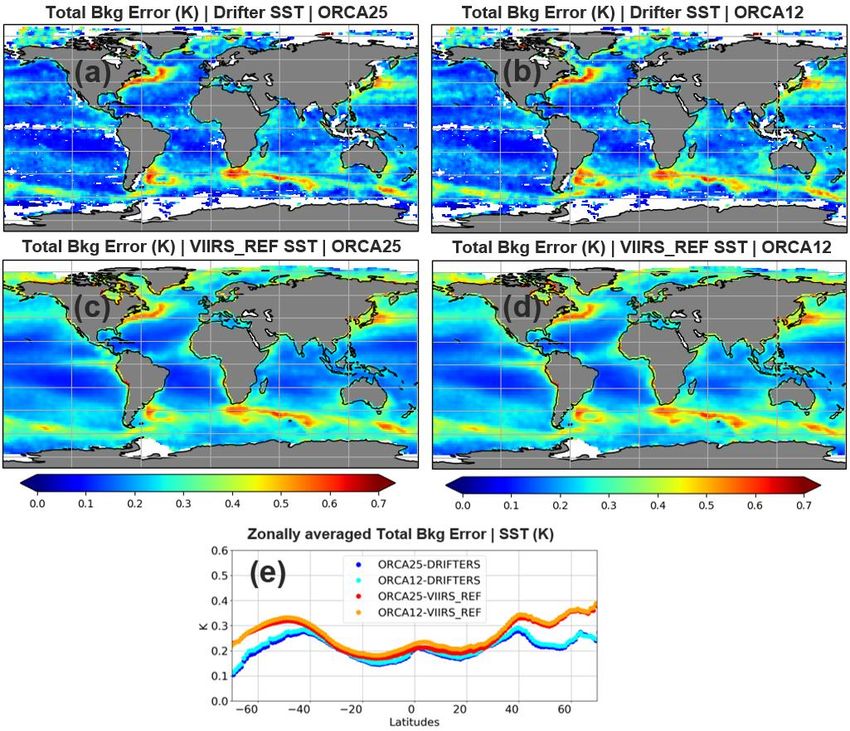
OFFICIAL-SENSITIVE

function fitting to produce isotropic estimates. It would be possible to also obtain the spatial
structures of the covariances in these different directions separately to estimate some
anisotropy (even if still aligned with the grid directions) but this is not done here. For
ORCA025/ORCA12/AMM15 we chose to use 25/100/500 grid-points in each direction giving
a maximum separation distance of about 700/900/750 km.

4. Results

4.1 Global error covariances

In this section we compare the forecast error covariances estimated by the HL and NMC
methods for ORCA025 and ORCA12 systems. The seasonal aspects of the forecast errors
and their respective length-scales are also evaluated based on error covariances estimated
over 2017-2018. The seasons are defined here as follows: December, January and February
(DJF); March, April and May (MAM); June, July and August (JJA); and September, October
and November (SON). The HL results are generated using a common grid and a common
specification of the separation distances for both model configurations.

4.1.1 Comparison of HL estimates between VIIRS and drifter innovations

In this section the HL estimates from VIIRS high-resolution satellite data are compared with
those estimated from in situ drifters. The similarities and discrepancies between these two
innovation datasets are evaluated and possible reasons for the differences are also discussed,
including the HL assumption about small-scale spatial correlations in the observation errors.
This assumption must be carefully checked for satellite data since correlations between them
may exist due to correlations along the scanning geometry and satellite swath, and due to
correlated errors in the atmospheric correction of the satellite retrieval. ORCA025 and
ORCA12 total background errors estimated from VIIRS innovations are compared in Fig. 4 to
those estimated from drifter buoy innovations. The representation of the main background
error features is consistent between the two innovation datasets. Both clearly show areas of
increased SST background errors within boundary current regions and the Antarctic
Circumpolar Current (ACC) for ORCA025 and ORCA12. Similar magnitudes of the
background errors can also be found in the subtropical gyres and tropical regions, which is
reinforced by the similar magnitudes of their zonal averages between 40°S and 40°N in Fig.
4e.
Nevertheless, differences in the SST background errors estimated from VIIRS and drifter
innovations can be spotted in coastal upwelling regions, such as along the western coast of
Africa, South and North Americas. Fig. 4e also shows that zonally averaged SST background
errors estimated by the two innovation datasets diverge towards high latitudes, particularly

OFFICIAL-SENSITIVE

poleward of 40°S and 40°N. These are approximately the latitudes where the number of VIIRS
and drifter observations begin to drop quite significantly (Fig. 5). This drop in the number of
observations matches quite consistently the increasing poleward differences between the SST
background errors estimated from VIIRS and drifters in Fig. 4e. As mentioned previously, the
robustness of HL error covariance estimates relies on the number of observations available.
If there are less VIIRS and drifter observations at high latitudes, one would expect greater
uncertainties around the estimation of HL error covariances, and therefore more significant
differences between the two innovation datasets are likely to appear there when compared to
lower latitudes.
Another relevant point to mention is that we only consider night-time VIIRS observations. As
a result, the number of VIIRS observations decreases at high latitudes in the summer
hemisphere where the daytime is extremely long. This results in HL error covariance estimates
that may be skewed towards winter results and therefore can be a factor contributing to explain
the discrepancies seen at high latitudes in Fig. 4e. Although this is perhaps not as relevant as
the points mentioned above, VIIRS and drifter measurements are done in different ways. While
drifters directly measure temperatures at depths of around 30 cm, VIIRS SSTs are originally
skin measurements. They need to be adjusted to represent the sub-skin through a thorough
calibration with drifters, which is a step performed by the data producers.

Figure 4: (a-d) 2017-2018 SST background errors (K) estimated by the HL method for drifters and VIIRS
observations, considering both ORCA025 and ORCA12 systems, respectively. The zonal averages of the SST
background errors for each global configuration and the respective observation types are shown in (e).

OFFICIAL-SENSITIVE

Figure 5: 2017-2018 number of SST observations (103) integrated for each latitude for drifters (top) and VIIRS
(bottom).

 4.1.2 Small-scale forecast error variances

After validating the HL SST background errors generated by VIIRS satellite data, the seasonal
aspects of the HL as well as the NMC background errors and their differences in both
ORCA025 and ORCA12 are evaluated. In order to understand the different characteristics of
the forecast errors, we decompose them into a small-scale component associated with the
mesoscale ocean variability and a large-scale component representing the background errors
that can occur over the scale of atmospheric synoptic systems (see section 3 for more details).
The magnitude of the former is shown for the summer and winter seasons in ORCA025 and
ORCA12, estimated by HL (Fig. 6) and NMC (Fig. 7) methods. Regardless of the seasons,
areas of increased small-scale background errors can be discerned in ocean regions with
large SST gradients, such as the Brazil-Malvinas Confluence (BMC), Gulf Stream and
Kuroshio current regions. This increase is also captured by the zonal averages of the small-
scale errors in both NMC and HL methods (Fig. 8), which peak at mid-latitudes where these
boundary currents are located.

© Crown copyright 2021, Met Office Page 19 of 48

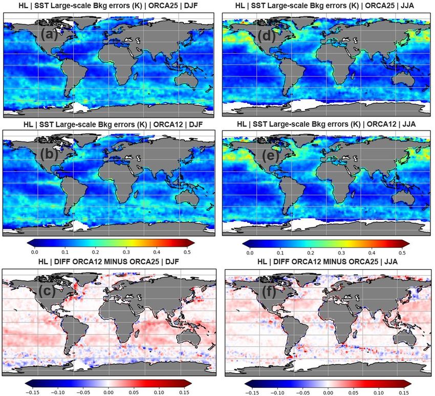
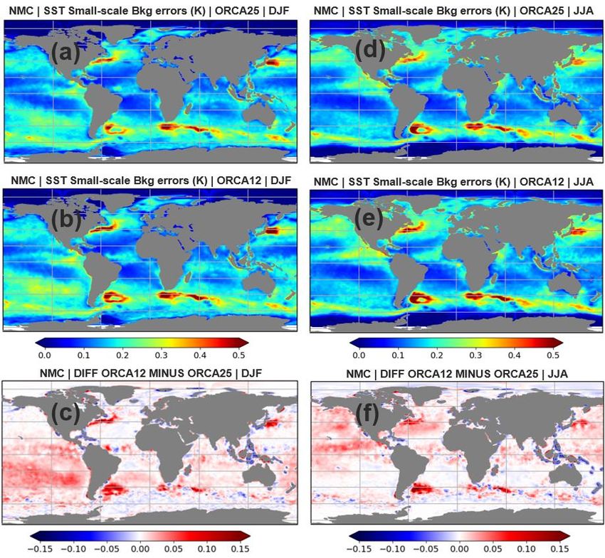
OFFICIAL-SENSITIVE

Figure 6: ORCA025 and ORCA12 small-scale SST background errors (K) estimated by the Figure 7: ORCA025 and ORCA12 small-scale SST background errors (K) estimated by the NMC
HL method using VIIRS observations for DJF (a-b) and JJA (d-e) seasons, respectively. method for DJF (a-b) and JJA (d-e) seasons, respectively. The differences between ORCA12 and
The differences between ORCA12 and ORCA025 for DJF and JJA are shown in (c) and (f), ORCA025 for DJF and JJA are shown in (c) and (f), respectively.
respectively.

 © Crown copyright 2021, Met Office Page 20 of 48

OFFICIAL-SENSITIVE

Although boundary currents are persistent features throughout all seasons, Figs. 6, 7 and 8
show a clear seasonal pattern of increased small-scale background errors in the summer
hemisphere, which is consistently seen in both error covariance methods and model
configurations. Roberts-Jones et al. (2016) found similar patterns of seasonal variability in
SST background errors estimated from the HL method. We agree with Roberts-Jones et al.
(2016) that a possible explanation for this is that the mixed layer depth (MLD) in both
hemispheres is shallower in summer months compared to winter. A shallower MLD in summer
leads to more sensitivity in the mixed layer due to wind and surface heat fluxes, which in turn
increase the SST variability. More localised seasonal patterns in the SST small-scale
background errors are also clearly picked up by the different methods and model
configurations in Figs. 6 and 7. For example, the Somali current in the Indian Ocean shows
enhanced SST small-scale background errors in JJA, which is consistent with the seasonality
caused by the Indian monsoon.

Figure 8: Zonal averages of HL (a-b) and NMC (c-d) small-scale SST background errors (K) for ORCA025 and
ORCA12, respectively. The error covariances in the HL method are estimated using VIIRS observations. The zonal
averages are calculated for DJF, MAM, JJA and SON seasons.

Even though similar seasonal patterns are reproduced across distinct model configurations,
some clear differences can be seen between ORCA12 and ORCA025 in both HL and NMC
methods for the small-scale background errors. In Figs. 6 and 7 ORCA12 produces larger SST
small-scale errors than ORCA025 almost everywhere, and this is clearly significant within the
boundary current regions for both DJF and JJA seasons. High-resolution models commonly
produce forecasts with seemingly realistic small-scale patterns that can be slightly misplaced.
Traditional point-matching verification measures would penalise such misplacements twice:
for not having the pattern where it should be, and for having a pattern where there should not
be one. For instance, when using neighbourhood methods for verification of the forecast
errors, Aguiar et al. (2021) found that ORCA12 performed better than ORCA025 if double
penalty effects are removed. The double penalty effects in ORCA12 SSTs might be explained

OFFICIAL-SENSITIVE

by the fact that ORCA12 resolves smaller scales, and it has larger SST gradients at those
scales than ORCA025. While SST observations are very high resolution and can constrain
those scales, the SLA observations are not as high resolution as the SSTs. Therefore, one
would expect that SLA assimilation is not able to constrain the same SST small-scale features,
and this might lead to an inability of the SST assimilation to properly constrain ORCA12 small-
scale features in the forecast results. This issue is exacerbated by the fact that the assimilation
in ORCA12 is performed on the ORCA025 grid, as described in Section 2.3. More results
about the small-scale component of the SST forecast errors in ORCA12 are discussed in
Section 4.1.5.
It is also interesting to note that differences in the small-scale background errors between
ORCA12 and ORCA025 follow a clear seasonal pattern in the NMC estimates and are larger
in summer compared to winter, particularly in the Pacific Ocean (Figs. 7c, f). The same pattern
is not obvious in the HL estimates (Figs. 6c, f). A possible explanation for this could be related
to diurnal cycle effects since the forecast difference for the NMC method is valid at 00 UTC,
which corresponds to the middle of the day in the Pacific Ocean. Errors at the peak of the
diurnal cycle are larger than other times of the cycle, and this becomes evident in summer
where the diurnal cycle is larger. In the HL technique the innovations only consider night-time
VIIRS observations and therefore the HL method only estimates the error covariances at night.
This might explain some of the discrepancies in the seasonal differences between ORCA12
and ORCA025 given by HL and NMC methods in the Pacific Ocean.

4.1.3 Large-scale forecast error variances

Figs. 9 and 10 show the large-scale component of ORCA025 and ORCA12 SST background
errors estimated from the HL and NMC methods, respectively. As in the small-scale
component of the SST errors, areas of increased large-scale errors are also found in the high
SST gradient regions, although their magnitude are smaller. Some of the mesoscale variability
in these regions may be accounted for in the large-scale error component, however as these
same regions encompass the storm tracks the increased errors could be a true large-scale
synoptic signal. The seasonal patterns in the large-scale component of the errors also closely
follow those from the small-scale component, with increased magnitudes in the summer
hemisphere. This seasonality is also reinforced by the zonal averages of the large-scale SST
background errors in Fig. 11. Regions with enhanced large-scale background errors are also
seen near India and Asia in JJA compared to DJF, which is consistent with the seasonal cycle
caused by the monsoons in these places. It is also worth noting that the spatial distribution of
the SST large-scale background errors is noisier compared to its small-scale counterpart. This
is probably due to the greater sensitivity of the function fitting to the large-scale component –
the signal is smaller at longer separation distances resulting in a smaller signal-to-noise ratio
there. Another explanation may be that the correlation structure is more anisotropic for the
large length-scales and therefore more difficult to fit with an isotropic function.

You can also read