Sensitivity of ecosystem-protected permafrost under changing boreal forest structures - AWI
←
→
Page content transcription
If your browser does not render page correctly, please read the page content below
LETTER • OPEN ACCESS

Sensitivity of ecosystem-protected permafrost under changing boreal
forest structures
To cite this article: Simone M Stuenzi et al 2021 Environ. Res. Lett. 16 084045

View the article online for updates and enhancements.

                              This content was downloaded from IP address 212.86.35.204 on 08/08/2021 at 10:02
Environ. Res. Lett. 16 (2021) 084045 https://doi.org/10.1088/1748-9326/ac153d
LETTER
Sensitivity of ecosystem-protected permafrost under changing
OPEN ACCESS
boreal forest structures
RECEIVED
31 March 2021 Simone M Stuenzi1,2,∗, Julia Boike1,2, Anne Gädeke6, Ulrike Herzschuh1,3,8, Stefan Kruse1,
REVISED Luidmila A Pestryakova7, Sebastian Westermann4,5 and Moritz Langer1,2
9 June 2021
1
ACCEPTED FOR PUBLICATION
Alfred Wegener Institute, Helmholtz Centre for Polar and Marine Research, Telegrafenberg A45, 14473 Potsdam, Germany
2
16 July 2021 Geography Department, Humboldt-Universität zu Berlin, Unter den Linden 6, Berlin 10099, Germany
3
Institute of Environmental Science and Geography, University of Potsdam, 14476 Potsdam, Germany
PUBLISHED 4
2 August 2021 Department of Geosciences, University of Oslo, Sem Sælands vei 1, 0316 Oslo, Norway
5
Centre for Biogeochemistry in the Anthropocene, University of Oslo, Sem Sålands vei 1, 0316 Oslo, Norway
6
Potsdam Institute for Climate Impact Research, Member of the Leibniz Association, Telegrafenberg, Potsdam 14412, Germany
Original Content from 7
Institute of Natural Sciences, North-Eastern Federal University in Yakutsk, Belinskogo str. 58, 677000 Yakutsk, Russia
this work may be used 8
under the terms of the Institute of Biochemistry and Biology, University of Potsdam, 14476 Potsdam, Germany
∗
Creative Commons Author to whom any correspondence should be addressed.
Attribution 4.0 licence.
E-mail: simone.stuenzi@awi.de
Any further distribution
of this work must Keywords: global warming impact, boreal forest, permafrost
maintain attribution to
the author(s) and the title
of the work, journal
citation and DOI.
Abstract
Boreal forests efficiently insulate underlying permafrost. The magnitude of this insulation effect is
dependent on forest density and composition. A change therein modifies the energy and water
fluxes within and below the canopy. The direct influence of climatic change on forests and the
indirect effect through a change in permafrost dynamics lead to extensive ecosystem shifts such as a
change in composition or density, which will, in turn, affect permafrost persistence. We derive
future scenarios of forest density and plant functional type composition by analyzing future
projections provided by the dynamic global vegetation model (LPJ-GUESS) under global warming
scenarios. We apply a detailed permafrost-multilayer canopy model to study the spatial
impact-variability of simulated future scenarios of forest densities and compositions for study sites
throughout eastern Siberia. Our results show that a change in forest density has a clear effect on the
ground surface temperatures (GST) and the maximum active layer thickness (ALT) at all sites, but
the direction depends on local climate conditions. At two sites, higher forest density leads to a
significant decrease in GSTs in the snow-free period, while leading to an increase at the warmest
site. Complete forest loss leads to a deepening of the ALT up to 0.33 m and higher GSTs of over
8 ◦ C independently of local climatic conditions. Forest loss can induce both, active layer wetting up
to four times or drying by 50%, depending on precipitation and soil type. Deciduous-dominated
canopies reveal lower GSTs compared to evergreen stands, which will play an important factor in
the spreading of evergreen taxa and permafrost persistence under warming conditions. Our study
highlights that changing density and composition will significantly modify the thermal and
hydrological state of the underlying permafrost. The induced soil changes will likely affect key
forest functions such as the carbon pools and related feedback mechanisms such as swamping,
droughts, fires, or forest loss.
1. Introduction insulate the underlying, ecosystem-protected perma-
frost (Chang et al 2015) and therefore play an import-
The boreal forest cover exerts a strong control on ant role in the development of boreal regions and the
numerous climate feedback mechanisms (Bonan et al stability of permafrost in a warming climate. Boreal
2018, Zhang et al 2018). Globally, 80% of boreal regions are projected to warm between 4 ◦ C and
forests are underlain by permafrost (Helbig et al 11 ◦ C by 2100, with a modest precipitation increase
2016). The forest cover is considered to efficiently (Scheffer et al 2012, Meredith et al 2019). The change
© 2021 The Author(s). Published by IOP Publishing LtdEnviron. Res. Lett. 16 (2021) 084045 S M Stuenzi et al
in air temperature and precipitation directly influ- Detailed modeling studies are needed to incor-
ences the vegetation cover development (Esper et al porate the local, heterogeneous, and complex feed-
2010, Kharuk et al 2015, Sato et al 2016, Ito et al 2020) back mechanisms, caused by the vegetation type
and permafrost thaw (Meredith et al 2019), directly and its relationship with topsoil temperature, act-
affecting soil water availability and root space lim- ive layer thickness (ALT), and available plant water
itation (Carpino et al 2018). The changing thermo- (Tchebakova et al 2009, Schuur and Mack 2018,
hydrological soil conditions may provoke changes Kropp et al 2021, Stuenzi et al 2021). It has been
in forest density and forest composition (Takahashi shown that the integration of ecosystem compon-
2006, Kharuk et al 2013, Liu et al 2017, Kropp et al ents such as permafrost is highly relevant for pro-
2021) leading to extensive ecosystem shifts (Pearson jections on biomass and vegetation cover (Ito et al
et al 2013, Gauthier et al 2015, Boike et al 2016, Kruse 2020). Here, we fill this gap between vegetation cover
et al 2016). model projections and the actual physical impact this
Forest composition and density exert a strong vegetation cover change has on permafrost ground,
control on permafrost stability (Yi et al 2007, and present a detailed coupled permafrost-multilayer
Chasmer et al 2011, Fisher et al 2016) and a direct canopy model, developed for use in permafrost-
feedback mechanism is expected to control the tem- underlain boreal forest systems.
poral ecosystem evolution (Bonan et al 1992, Carpino We analyze (a) the trends of the two ecosystem
et al 2018, Loranty et al 2018). This feedback mech- changes, boreal forest densification and plant func-
anism (figure A1) is, however, poorly understood and tional type composition, based on biome LPJ-GUESS
broad-scale vulnerability studies do not yet exist. The model projections for north-eastern Siberia. Based
canopy exerts shading by reflecting and absorbing on the projected trends in ecosystem changes, we
most downward solar radiation and by suppressing use CryoGrid to simulate the projected ranges of (b)
the majority of turbulent heat fluxes in the below- forest densities and (c) plant functional type com-
canopy space (Chang et al 2015). Further, the canopy positions for three different study sites throughout
controls the surface albedo, which is much lower than north-eastern Siberia to investigate the impact of can-
in grasslands especially during snow-covered periods opy variability on the ground thermal and hydro-
(Bonan and Shugart 1989). The canopy decreases soil logical regime. We thereby study the effect of the
moisture and leads to a reduced thermal conductiv- projected trends over an extensive range of predom-
ity through precipitation interception (Thomas and inantly deciduous-dominated boreal forests, as well
Rowntree 1992) and higher evapotranspiration (Vitt as over different climate characteristics within the
et al 2000). Additionally, the canopy slows snow melt- polar climate regime. This study delivers important
ing in spring and reduces snow compaction because insights into the range of spatial differences and pos-
of the suppressed turbulent fluxes, which therefore sible temporal changes to the permafrost condition
leads to higher snowpacks under denser canopies that can be expected following landscape changes
(Stuenzi et al 2021). Finally, the vegetation cover such as deforestation through fires or other anthro-
promotes the accumulation of an organic surface pogenic influences, afforestation in currently unfor-
layer (Bonan and Shugart 1989, Yi et al 2007) which ested grasslands, or the climate-induced densification
further insulates the topsoil from the atmosphere. of forested areas.
A change in the forest density modifies the within-
and below-canopy energy and water fluxes (Chasmer 2. Methods
et al 2011, Stuenzi et al 2021). The forest composi-
tion also has an impact on the ground surface energy 2.1. Study region
and water balance. Most boreal forests are dominated The treeline of north-eastern Siberia is dominated
by evergreen needleleaf taxa, but wide areas of the by the deciduous needleleaf tree genus Larix Mill.
north-eastern Eurasian continent are dominated by (figure 1), even though in mixed forest stands, larch
deciduous needleleaf taxa. The needle-shedding of taxa are out-competed by evergreen taxa, which
deciduous taxa impacts the within and below canopy is thought to represent the late-successional stage
fluxes (Tanaka et al 2008, Zhang et al 2011, Peng et al (Kharuk et al 2007). Once established, larch forests
2020, Stuenzi et al 2021), the litter and organic surface are likely to stabilize through a complex vegetation-
layers (Bonan and Shugart 1989) and the fire regime permafrost-climate feedback system. Mainly shal-
(Rogers et al 2015). Since evergreen and deciduous low active layer depths hinder the establishment
taxa can establish under similar climate conditions of evergreen taxa (Herzschuh 2019) and in more
(Esper and Schweingruber 2004, Kharuk et al 2009) southern regions of eastern Siberia, larch is mixed
the successful spread of evergreen taxa into currently with evergreen conifers (pine, spruce, fir) and hard-
larch dominated areas and vice-versa, mainly depends woods (Kharuk et al 2019). The ground vegetation
on the frequency of disturbance events, which have is generally dominated by mosses and lichens that
increased over the past decades (Shuman et al 2011, form carpets. Larch has shallow roots and preferably
Mekonnen et al 2019, Meredith et al 2019). grows on clay permafrost soils with a shallow ALT and
2Environ. Res. Lett. 16 (2021) 084045 S M Stuenzi et al
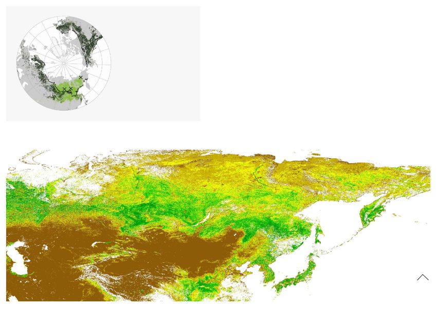
Figure 1. Main map: leaf area index (m2 m−2 ) from satellite imagery and permafrost extent in north-eastern Siberia. The three
study sites are marked with black crosses (Nyurba (NYU), Spasskaya Pad (SPA), and Chukotka (CHK)). Additionally, the dotted
line indicates the two individual study regions, West (E 105.25◦ –137.25◦ ) and East (E 137.75◦ –169.75◦ ) as used in the biome
projection data analysis. Top left corner: spatial distribution of current deciduous and evergreen boreal forest dominance and the
study sites. Data: ESA CCI Land Cover classes. ESA. Land Cover CCI Product User Guide Version 2. Tech. Rep. (2017) (after
(Herzschuh 2019)), permafrost extent from Land Resources of Russia—Maps of permafrost and Ground Ice (after Kotlyakov and
Khromova (2002)), and Copernicus Global Land Service, Leaf Area Index (LAI), (after Copernicus Global Land Operations
(2021)). Adapted from Stuenzi et al (2021). CC BY 4.0.
maximum wetness of 20%–40%. Evergreen conifers (2014). The model is forced with bias-adjusted cli-
and hardwood both prefer deeper active layers and mate data from the Hadgem2-es earth system model.
a higher soil moisture availability (Ohta et al 2001, The EWEMBI dataset (Lange 2019) served as the
Rogers et al 2015). To capture these spatial differences basis for the trend-preserving bias adjustment of
across boreal forests, we study the current forest com- the GCMs at a daily time step (as detailed in Fri-
position and structure along a east-west transect rep- eler et al (2017)). The data selected cover a region
resented by three different sites as specified in table 1, from E 105◦ –167◦ and N 45◦ –70◦ at a spatial res-
figure 1, and appendix B with figure B1. olution of 0.5◦ × 0.5◦ . We have separated this area
into two individual study regions: West (E 105.25◦ –
2.2. Projected forest evolution 137.25◦ ) and East (E 137.75◦ –169.75◦ ) (figure 1),
We use ESA CCI Land Cover satellite data to para- because of the differences in temperature and cur-
meterize forest composition and Copernicus Global rent vegetation cover between these two regions. We
Land Service leaf area index (LAI) data to paramet- analyze projected LAI for needleleaf evergreen and
erize forest density under current climate conditions needleleaf deciduous plant functional types under the
(figure 1). To understand the current plant functional three warming scenarios at the transect sites. Note
type distribution and the projected changes we study that these LAI values are averaged annual values over
projections of LAI and plant functional types simu- the entire study sites, and do not represent the full
lated by the LPJ-GUESS model as part of ISIMIP2b summer LAI in deciduous forests. Therefore, we also
(Frieler et al 2017). We analyze the forest change study the projected monthly LAI (only available for
scenarios from 2006 until 2099 under three global the combination of all PFTs) for August, which cor-
warming scenarios (RCP 2.6, RCP 6.0, RCP 8.5). The responds to the maximum LAI of deciduous taxa plus
LPJ-GUESS dynamic vegetation model combines an the LAI of all other PFTs, including needleleaf ever-
individual- and patch-based representation of forest green and hardwoods, under the available warming
dynamics with biogeochemical cycling from regional scenarios (RCP 6.0, RCP 8.5) for the period 2006–
to global scales and is further described in Smith et al 2099 (figure B2).
3Environ. Res. Lett. 16 (2021) 084045 S M Stuenzi et al
Table 1. Description of different study sites. Adapted from Stuenzi et al (2021). CC BY 4.0.
Study site Nyurba (NYU) Spasskaya Pad (SPA) Chukotka (CHK)
Lat N 63.08◦ N 62.14◦ N 67.40◦
Lon E 117.99◦ E 129.37◦ E 168.37◦
Elevation (m asl) 117 237 603
Mean annual air temperature (◦ C) −3.69 −5.97 −11.69
Mean snow-covered air temperature (◦ C) −9.6 −12.7 −17.7
Mean snow-free air temperature (◦ C) 13.6 13.7 6.0
Solid precipitation (mm) 101 84 116
Liquid precipitation (mm) 180 170 292
Dominant plant functional type Evergreen Deciduous Deciduous
Tree height (m) 8 12 11
Leaf area index (m2 m−2 ) 3 3 1
Study regions West West East
2.3. Coupled permafrost-vegetation model precipitation, incoming long- and shortwave radi-
The model setup is based on the permafrost model ation, and cloud cover) are obtained from ERA-
CryoGrid (originally described in Westermann et al Interim (ECMWF Reanalysis) extracted for the three
(2016)), a one-dimensional, numerical land surface sites (N 63.08◦ , E 117.99◦ , N 62.14◦ , E 129.37◦ , and
model that simulates the thermo-hydrological regime N 67.40◦ , E 168.37◦ ) (Simmons et al 2007). We use
of permafrost ground by numerically solving the ground surface temperature (GST, top 0.4 m of the
heat-conduction equation (Nitzbon et al 2019). The soil column) as the major target variable for model
CryoGrid model was extended by a multilayer can- validation (appendix D). We further analyze max-
opy module developed by Bonan et al (2014) for imum yearly ALT and the available water for plants
the use in permafrost regions (appendix C and Stu- within this active layer (PAW).
enzi et al (2021) for model details). Here, we add For each study site, we conduct 70 simulations
a parameterization for deciduous forest to simulate representing different forest types and forest compos-
the leafless state of deciduous-dominated regions out- itions (figure 2). The range of different forest types
side of the short vegetative period in summer. This is considered are bench-marked based on the projec-
achieved by allowing for separate leaf area index con- ted ISIMIP2b data described by canopy density (leaf
trolled by static time windows defining leaf-on and area index, LAI (m2 m−2 )) between 0 and 7 m2 m−2
leaf-off season (10 October–10 April) following liter- and fractions between deciduous needleleaf and ever-
ature values for east Siberia (Spasskaya Pad) (Ohta green needleleaf taxa (0%–90% deciduous) (figure 2).
et al 2001). Further, a more realistic canopy struc- To test the statistical significance of the differences
ture is simulated by allowing fractional composition between the simulated mean GSTs for varying forest
of deciduous and evergreen taxa within the simu- densities and compositions, we apply variance ana-
lated forest stand. In addition, we test a parameter- lysis (one-way ANOVA) with a significance level of
ization for coupling forest density (LAI) to fine root 0.001. Data are controlled for normal distribution
biomass (Rtotal , (gm−2 )) (appendix D). Further, we and homogeneous variance across all groups. Stat-
have implemented a new relationship for phase parti- istical analyzes were performed using R software (R
tioning of water in frozen soil (freeze curve) based on Core Team 2016).
Painter and Karra (2014) (appendix C).
3. Results
2.4. Model simulations and setup
We ran model simulations for a wide range of forest 3.1. Forest evolution under climatic warming
types and forest compositions at the three transect The biome projection data from LPJ-GUESS model
sites. Parameters defining the canopy, snow, and simulations data reveal that in the eastern sub-
soil properties were set according to literature val- domain of our study region an increase in evergreen
ues, model documentation, and own measurements taxa are projected for all warming scenarios (RCP
(appendix for details). Tables E2 and E4 summar- 2.6, RCP 6.0, RCP 8.5), with a peak in the yearly
ize the ground and vegetation parameter choices mean value of 0.5 m2 m−2 and a maximum value of
for all three sites. Table E3 summarizes constants 2 m2 m−2 , and 1.8 m2 m−2 around 2075 respectively,
used. We perform model simulations over a time for the RCP 6.0 and RCP 8.5 scenarios, followed by
period of five years from August 2014 to August 2019. a decrease towards the end of the century (figure 3).
This equals a spin-up period of four years before In the western sub-domain, the three global warming
comparing modeled and measured data. The met- scenarios project an increase in deciduous taxa. The
eorological forcing data (air temperature, air pres- overall LAI for August under the RCP 8.5 warming
sure, wind speed, relative humidity, solid and liquid scenario increases by 2 m2 m−2 in the western region
4Environ. Res. Lett. 16 (2021) 084045 S M Stuenzi et al
Figure 2. Schematic of the simulated vegetation trajectories and the possible impact on the thermal development of the
permafrost. Left: photographs from the three study sites and the respective model set-ups for Nyurba (NYU), mixed forest with a
LAI of 3 m2 m−2 (mid-density), for Spasskaya (SPA), deciduous-dominated forest with a LAI of 3 m2 m−2 (mid-density), and for
Chukotka (CHK), deciduous-dominated with a LAI of 1 m2 m−2 (low-density). Right: schematic illustration of the range of
possible forest cover scenarios (Forest density: low-density to high density, and forest composition: evergreen, mixed (10%–50%
of deciduous taxa) or deciduous dominated (60%–90% of deciduous taxa), and no forest cover) caused by either, climatic
changes and/or disturbance events such as i.e. an extreme drought, a fire event, logging, or pest infestation. Each forest cover
scenario is simulated at each of the three sites, NYU, SPA and CHK.
Figure 3. Projected LAI for needleleaf evergreen (blue) and needleleaf deciduous (red) plant functional types under the three
warming scenarios, RCP 2.6, RCP 6.0, and RCP 8.5 for the time frame 2006–2099. Data covers the region from E 105◦ − 167◦ to
N 45◦ − 70◦ and is separated into two individual study regions, West (E 105.25◦ –137.25◦ , bottom) and East (E 137.75◦ –169.75◦ ,
top). The lines indicate mean values while the shaded areas show the corresponding 90th and 10th percentile.
5Environ. Res. Lett. 16 (2021) 084045 S M Stuenzi et al
Figure 4. Averaged modeled snow-covered period GST, average modeled snow-free period GST and the respective spread for
different forest canopy densities (LAI = 2 − 7 m2 m−2 ) and no forest cover (LAI = 0 m2 m−2 ) at the three study sites over 1 year
(10 August 2018–10 August 2019). Statistical significance of each trend is based on ANOVA analysis (significance codes: ∗∗∗ =
0.001, ∗∗ = 0.01, ∗ = 0.05). The bars indicate mean values while the whiskers show the corresponding standard deviations.
and doubles in the eastern region (appendix B). Cur- temperatures under all warming scenarios and for
rently, we find mean values around 3 m2 m−2 for both study regions.
the western study region and 1 m2 m−2 in the east.
According to the annual data (figure 3), the mean 3.2. Permafrost sensitivity under changing forest
LAI is currently dominated by evergreen taxa. In the density
western region, this dominance switches around 2050 The simulations clearly demonstrate that higher
under all three climate forcing scenarios. Under the forest density leads to lower mean GST in the snow-
strongest climatic warming scenario, deciduous LAI free period. This trend is highly significant with p <
increases to a mean value of 2.4 m2 m−2 , a value three 0.01 for Chukotka and Nyurba. The average snow-
times higher than the end of the century decidu- free GST is 1 ◦ C colder for the simulations with
ous taxa projection under RCP 2.6. The projection the densest canopy covers. For Spasskaya Pad (SPA),
data reveals an increase in needleleaf evergreen taxa this trend is reversed, showing an increasing GST
at both sites for the coming decade, followed by a for denser canopies (p < 0.01). In the snow-covered
decrease in the western region under all climate scen- period mean GST increase with larger LAI values at
arios. In the eastern region, the increase continues Chukotka and Nyurba (p < 0.01) (figure 4). Tem-
until 2060, where-after the LAI of needleleaf ever- perature values for the simulations without forest are
green taxa stays constant under RCP 2.6 and decreases higher at all sites and for both time periods except for
under both the RCP 6.0 and 8.5 scenarios. In the the snow-covered period at the Nyurba site, where the
western region, deciduous taxa will continue increas- simulation without forest cover is 1.3 ◦ C colder. The
ing until the end of the century under all climate maximum difference between a sparse forest cover
forcing scenarios. Based on these data, which are in and no forest cover is a temperature increase of 8.3 ◦ C
agreement with other model projections for Eurasia in the snow-covered period at Chukotka.
(Shuman et al 2014, Meredith et al 2019), we can Our model simulations show that the projected
constrain the expected changes in plant functional forest development alone exerts a strong control on
type compositions and forest densities for the entire the thermal state of the permafrost, in addition to the
eastern Siberian permafrost underlain boreal forest expected effect of a warmer and dryer climate itself. At
region east of 105◦ and north of 45◦ . The overall two study sites, higher forest density leads to a signi-
forest density is projected to increase with warming ficant decrease in ground surface temperatures in the
6Environ. Res. Lett. 16 (2021) 084045 S M Stuenzi et al
Figure 5. Top: Averaged modeled maximum ALT and the spread for different forest canopy densities (LAI = 2 − 7 m2 m−2 ) and
no forest cover (LAI = 0 m2 m−2 ) at the three study sites over 1 year (10 August 2018–10 August 2019). Bottom: total modeled
available plant water in the ALT and the spread for different densities (LAI = 2 − 7 m2 m−2 ) and no forest cover (LAI =
0 m2 m−2 ) at the three study sites over 1 year (10 August 2018–10 August 2019). Statistical significance of each trend is based on
ANOVA analysis (significance codes: ∗∗∗ = 0.001, ∗∗ = 0.01, ∗ = 0.05). The bars indicate mean values while the whiskers show
the corresponding standard deviations.
snow-free period, while leading to an increase at the Here, the average maximum ALT of all simulations
warmest site, SPA. at highest forest density (7 m2 m−2 ) is 0.22 m, while
The magnitude of the insulation effect on the average ALT is 0.27 m for a low LAI (1 m2 m−2 ). The
annual GST change from no forest cover to a dense maximum ALT under a dense forest canopy is thus
forest cover is −6.3 ◦ C at Chukotka, −0.2 ◦ C at found 0.05 m (−19%) lower than under a sparse can-
Nyurba, and −2.5 ◦ C at Spasskaya. opy. At Nyurba we find an average maximum ALT
The impact of forest density on GST consequently value of 0.45 m for a sparse canopy as well as for a
alters the annual ALT dynamics. We find a decline dense canopy. At SPA low-density forest results in
in maximum ALT with increasing canopy density for a maximum ALT of 0.54 m, which is considerably
two sites in our study region. Highest maximum ALT lower than the mean value of 0.57 m (−5%) for high-
of 0.68 m is found at the Spasskaya site with a LAI of density forest.
0 m2 m−2 . The lowest maximum ALT is simulated at In order to analyze the impact of forest density on
the Chukotka site with a value of 0.2 m only for LAI soil hydrology, we investigate the total yearly avail-
7 m2 m−2 (figure 5). We find a significant trend (p < able plant water within the active layer. We find a
0.01) of a decrease in ALT with an increasing can- clear and significant trend at Chukotka and Nyurba,
opy density in Chukotka but an insignificant trend with a decrease in available plant water for higher
in Nyurba. At the SPA site, our model predicts an forest densities. The Chukotka site reveals the avail-
increasing maximum ALT with an increasing canopy able plant water to be three times higher for the sim-
density from LAI 1 − 4 m2 m−2 . The maximum ALT ulation without forest cover. The soil moisture in the
for the simulations without a forest cover is higher at active layer steadily decreases with increasing forest
all sites. The difference between LAI 1 m2 m−2 and no density at Chukotka and Nyurba, whereas it remains
forest cover is up to 0.33 m in Chukotka. The decrease constantly low for SPA. SPA is the driest site, both in
in snow-free period insulation with higher forest terms of liquid and solid precipitation, which leads to
density is strongest at the coldest site of Chukotka. a very low amount of available plant water together
7Environ. Res. Lett. 16 (2021) 084045 S M Stuenzi et al
Figure 6. Averaged modeled snow-covered period GST, average modeled snow-free period GST and the respective spread for
different percentages of deciduous taxa (90%–0%) at the three study sites over 1 year (10 August 2018–10 August 2019). Statistical
significance of each trend is based on ANOVA analysis (significance codes: ∗∗∗ = 0.001, ∗∗ = 0.01, ∗ = 0.05). The bars indicate
mean values while the whiskers show the corresponding standard deviations.
with a relatively shallow snow cover (< 0.2 m) during the summer period is found at SPA and Chukotka
winter. (p < 0.01).
The available plant water found is up to four The magnitude of the insulation on the annual
times higher for the non-forested simulation at the GST change from evergreen to deciduous forest cover
Chukotka site and up to two times higher at the is −2.3 ◦ C at Chukotka, −0.3 ◦ C at Nyurba, and
Spasskaya site. This indicates that forest loss may −1.2 ◦ C at Spasskaya.
trigger the development of wetter and potentially Changes in deciduousness also affect maximum
swampy soil conditions depending on precipitation, ALT and the available plant water (figure 7). At SPA,
evaporation, and ALT. In contrast, forest cover loss Chukotka and Nyurba we find statistically signific-
leads to a reduction in available plant water (up to ant trends (p < 0.01) towards higher maximum ALTs
50%) at Nyurba which is characterized by climate with decreasing deciduous taxa. The difference in ALT
conditions similar to Spasskaya. These contrasting between 90% and 0% deciduous taxa are +0.04 m
hydrological impacts were observed in the vicinity of (+15%) at Chukotka, +0.05 m (+11%) at Nyurba
the respective study sites of Spasskaya and Nyurba. and +0.07 m (+11%) at SPA. We find statistically
The performed simulations, thus, reveal that boreal significant trends (p < 0.01) towards higher avail-
forest loss can amplify both the wetting and drying of able plant water with decreasing deciduous taxa at
sub-Arctic regions. Chukotka and Spasskaya.
3.3. Permafrost sensitivity under changing forest 4. Discussion
composition
Across the three study sites, we find a significant About 55% of the total global permafrost area is
trend (p < 0.01) in lower GST’s with an increasing covered by boreal forest (Gruber 2012, Helbig et al
percentage of deciduous taxa in the snow-covered 2016). The forest cover plays an important role in
period (figure 6). A lower percentage of deciduous insulating and stabilizing the permafrost underneath.
taxa leads to a significant increase in the mean win- The magnitude of this is highly dependent on the
tertime GST at Chukotka and Nyurba. The forest forest density as well as on the forest composition and
enhanced insulation effect of evergreen canopies, structure but this relationship has not yet been stud-
compared to deciduous cover, reaches up to +2.7 ◦ C ied in depth (McGuire et al 2002, Fisher et al 2016,
during the snow-covered period at Chukotka. A cool- Stuenzi et al 2021). Our results provide a detailed
ing trend of lower percentages of deciduous taxa in examination of the exact impact of boreal forest on
8Environ. Res. Lett. 16 (2021) 084045 S M Stuenzi et al
Figure 7. Top: Averaged modeled maximum ALT and the spread for different percentages of deciduous taxa (100%–0%) at the
three study sites over 1 year (10 August 2018–10 August 2019). Bottom: Total modeled available plant water in the ALT and the
spread for different percentages of deciduous taxa (90%–0%) at the three study sites over 1 year (10 August 2018–10 August
2019). Statistical significance of each trend is based on ANOVA analysis (significance codes: ∗∗∗ = 0.001, ∗∗ = 0.01, ∗ = 0.05).
The bars indicate mean values while the whiskers show the corresponding standard deviations.
permafrost by covering a wide variety of forest dens- to the previously described change in fire regime
ities and plant functional type compositions. (Rogers et al 2015) and albedo decrease (Bonan and
We find forest density to significantly control the Shugart 1989), the lower insulation capacity of ever-
ground thermohydrological conditions at all sites, green canopies will be an important factor in the
whereby trends strongly differ in magnitude and dir- spreading of evergreen taxa in eastern Siberia. The
ection. The cooling trends of denser canopies at the actual thermal and hydrological impact of the forest
wetter sites, and the warming trend at the driest site, cover is therefore determined by the forest density and
are reflected in the ALT dynamics. At the coldest site, structure, highly dependent on the local climate and
the maximum ALT under a dense canopy is 19% hydrological conditions, and therefore varies greatly
lower than under a sparse canopy. Forest loss leads between our study sites. We find that forest loss can
to higher snow-free GSTs at all sites and higher snow- amplify wetting as well as drying of the soil. The
covered GST at Chukotka and Spasskaya, with a max- available plant water after forest cover loss is four
imum temperature increase of +8.3 ◦ C. In just five times higher at the coldest site, two times higher at
years the forest cover loss leads to a warming of the the warmest site, and 50% reduced at the driest site.
GSTs at the same order of magnitude as the projected Depending on precipitation and soil type, forest cover
temperature increase for boreal regions 4 ◦ C–11 ◦ C loss can induce both drying and wetting. Generally,
until 2100 (Meredith et al 2019). In the snow-covered the reduction in transpiration after forest loss leads
period, a lower share of deciduous trees was found to wetter soils (O’Donnell et al 2011, Loranty et al
to lead to warmer GSTs at all three sites. This differ- 2018) which we find at both Spasskaya and Chukotka.
ence in insulation capacity between deciduous- and A further important factor determining the hydrolo-
evergreen-dominated canopies is up to +2.7 ◦ C at the gical conditions is the nature of the soil type (Boike
Chukotka site and +1.5 ◦ C at SPA. Deciduousness has et al 2016, Loranty et al 2018, Holloway et al 2020).
a higher effect on the average GSTs in cold regions Very sandy soils explain the good draining conditions
(Chukotka) and a significant effect on the snow- and the resulting drying trajectory at Nyurba, while
covered GSTs at all sites. We show that in addition the clay-containing soils at Spasskaya and Chukotka
9Environ. Res. Lett. 16 (2021) 084045 S M Stuenzi et al
are drained less, and hence the forest cover change can 2021). Here, we show that these changes will cause a
lead to wetting. shift in the thermal and hydrological permafrost state,
In this study, we focus on the direct physical which potentially destabilizes tightly coupled ecosys-
impact of forest change on the detailed thermal tem functions.
and hydrological conditions of permafrost ground
underneath, rather than investigating the exact tim- 4.1. Conclusions
ing of these ecosystem changes because the simula- In this study, we can underlay the tightly coupled
tions themselves are decoupled from projected cli- interplay between forest and permafrost development
mate forcing data. Because of the difference found in with a physically-based model and make predictions
the forest cover’s impact on the thermal regime of the on the progression of ecosystem-protected perma-
permafrost ground, we argue, that specific, local and frost under a variety of forest change scenarios. In
detailed land-surface models are needed to under- summary, we identify the following key points:
stand the complex dynamics in permafrost underlain
boreal ecosystems. Further, higher detail in the sim- (a) A change in forest density clearly affects the
ulated change to the thermal and hydrological condi- ground surface temperatures at all sites. Tem-
tions could be achieved by incorporating a change in perature differences are highest at the coldest
the thickness or composition of the litter, moss, and site and in the snow-free period. This is further
organic layers over time, and by additionally simu- reflected by a decrease in the maximum ALT of
lating the plant functional type broadleaf, which can up to 0.05 m or 19% at the two colder sites. The
establish wherever sufficient precipitation is available direction of this trend highly depends on local
(Kharuk et al 2009, Shuman et al 2011). climate conditions.
While knowledge about carbon sequestration (b) At all sites, simulations without a forest cover
through boreal forests is well-established, more and reveal higher maximum ALTs of up to 0.33 m and
more studies have found that different processes higher GSTs of more than 8 ◦ C after only five
can counteract the boreal forest’s role as a carbon years. The thermal impact of forest cover loss is
sink (Betts 2000, Bonan 2008). As such, a decreas- on the same order of magnitude as the climate
ing albedo due to afforestation has been found to warming projected for the region until 2100.
lead to a positive climate forcing for certain regions Complete forest loss is found to lead to a deepen-
(Bonan 2008, Stuenzi and Schaepman-Strub 2020). ing of the ALT and a warming of GSTs at all sites,
Further, forest loss can lead to reduced evapotran- independent of local climatic conditions.
spiration and a resulting short-term positive forcing (c) Depending on precipitation and soil type, forest
effect (Liu et al 2019), as well as to an increased cover loss can induce both drying and wetting.
surface albedo, mainly in the snow-covered-period, After forest cover loss, the available plant water
and hence, a strong cooling effect (Lyons et al 2008, is four times higher at the coldest site, two times
Rogers et al 2015, Chen et al 2018, Liu et al 2019). higher at the warmest site, and 50% reduced at
We argue that the development of the forest cover the driest site.
does not only influence the future of the boreal forest’s (d) At all sites, deciduous dominated canopies reveal
function as a carbon sink but also plays an import- lower GSTs, especially during the snow-covered
ant role in the stability of permafrost. We show that period. This difference in insulation capacity
varying density and tree composition have a signi- reaches up to +2.7 ◦ C for pure evergreen stands
ficant effect on the thermal and hydrological state and is likely an important factor controlling the
of permafrost. The insulating effect of the forest spreading of evergreen taxa and controlling the
cover depends on the local climatic conditions but resilience of ecosystem-protected permafrost.
significant impact was found at all sites. Finally,
the structure and composition of forests are highly In the light of increasing disturbances (such as
dependent on the local ecosystem resilience towards fires and diseases) in boreal forests our conclu-
an increasing frequency and intensity of forest fires, sions have strong implications regarding permafrost-
rising air temperatures, and a decrease in precipita- vegetation-climate feedback mechanisms. Our sim-
tion (Shuman et al 2011, Mekonnen et al 2019). Espe- ulations indicate a positive feedback between the
cially, the favoring of different fire regimes between successive establishment of evergreen taxa and active
evergreen and deciduous taxa, as well as warmer layer deepening which may accelerate further forest
and drier conditions, can lead to fast ecosystem transformation and permafrost thaw. In addition,
shifts. Altered thermal conditions, soil drainage or forest cover transformation will have a strong impact
higher soil wetness, enrichment in nutrients, and an on the hydrological regime, which may further amp-
increased active layer depth can all have a favoring lify climate-induced changes in near surface temper-
effect on either evergreen needleleaf or deciduous ature and precipitation. In consequence, the feed-
hardwood expansion, lead to the complete loss of back loop might be further amplified by increasing
forest cover, or change the forest density (Takahashi fire probability and disease vulnerability due to addi-
2006, Kharuk et al 2013, Liu et al 2017, Kropp et al tional water stress. On the other hand, under wetter
10Environ. Res. Lett. 16 (2021) 084045 S M Stuenzi et al
climate conditions, enhanced wetting can eventually from AG, Kirsten Thonicke, Christopher Reyer and
lead to swamping and thermokarst causing forest die- Martin Gutsch in acquiring the land cover projec-
back as observed in drunken forests. tion data. Further, SMS is very grateful for the help
SMS designed the study, developed and imple- during fieldwork in 2018 and 2019, especially for the
mented the numerical model, carried out and ana- help from Levina Sardana Nikolaevna, Alexey Nikola-
lyzed the simulations, prepared the results figures and jewitsch Pestryakov, Lena Ushnizkaya, Luise Schulte,
led the paper preparation. ML, SW, JB, UH and SK Frederic Brieger, Stuart Vyse, Elisbeth Dietze, Nadine
co-designed the study, and supported the interpret- Bernhard, Boris K. Biskaborn, Iuliia Shevtsova, as well
ation of the results. SMS, ML, and SW implemented as Luidmila Pestryakova and Evgeniy Zakharov. Addi-
the code in the model and designed the model simu- tionally, SMS would like to thank Stephan Jacobi,
lations. AG prepared the land cover projection data. Alexander Oehme, Niko Borneman, Peter Schreiber
SMS, UH and SK prepared and conducted the field and William Cable for their help in preparing for field
work in 2018, SMS conducted the field work in 2019. work and the entire PermaRisk and Sparc research
SMS wrote the paper with contributions from all co- groups for their ongoing support.
authors. UH, ML and JB secured funding. This study has been supported by the ERC con-
No competing interests are present. solidator grant Glacial Legacy to Ulrike Herzschuh
(No. 772852). Further, the work was supported by the
Data availability statement Federal Ministry of Education and Research (BMBF)
of Germany through a grant to Moritz Langer (No.
The code is available on Zenodo (DOI: https:// 01LN1709A). Funding was additionally provided by
doi.org/10.5281/zenodo.4603.668). The iButton soil the Helmholtz Association in the framework of
temperature data are available at https://doi.org/ MOSES (Modular Observation Solutions for Earth
10.1594/PANGAEA.914327 (Langer et al 2020). The Systems). Luidmila A. Pestryakova was supported by
AWS data are available at https://doi.pangaea.de/ the Russian Foundation for Basic Research (Grant
10.1594/PANGAEA.918074 (Stuenzi et al 2020). No. 18-45-140053 ra) and Ministry of Science and
Higher Education of Russia (Grant No. FSRG-2020-
Acknowledgments 0019). Sebastian Westermann acknowledges fund-
ing by Permafost4Life (Research Council of Nor-
SMS is thankful to the POLMAR graduate school, way, Grant No. 301639) and ESA PermafrostCCI (cli-
the Geo.X Young Academy and the WiNS program mate.esa.int/en/projects/permafrost/). AG received
at the Humboldt University of Berlin for providing a funding by the German Federal Ministry of Education
supportive framework for her PhD project and help- and Research (BMBF) and the European Research
ful courses on scientific writing and project man- Area for Climate Services ERA4CS with project fund-
agement. SMS would like to acknowledge the help ing reference 518, No.01LS1711C (ISIPedia project).
11Environ. Res. Lett. 16 (2021) 084045 S M Stuenzi et al
Appendix A. Interactions between the atmosphere, boreal forest and permafrost
Figure A1. Interactions between the atmosphere, boreal forest cover, and permafrost. In red (energy) and blue (hydrology) are all
the mechanisms changing due to climatic changes. Climatic change leads to a change in the forest density and structure, which
leads to changes in all feedback processes between forest and permafrost. Additionally, climatic change leads to permafrost
thawing and a change in the water availability, which also leads to forest density and structure changes.
Appendix B. Study sites and their climate (Ohta et al 2001, Maximov 2015). SPA is located in
a continuous permafrost region, and the active-layer
B.1. Study sites depth is around 1.2 m in larch-dominated forests. The
B.1.1. Nyurba soils are sandy loam, and nutrient-poor. The forest
The most western study site is located south east of soil has a litter layer of 0.08 m and an A-horizon
Nyurba at N 63.08◦ , E 117.99◦ , and 117 m asl, in a reaching a depth of 0.16 m, mineral soil is podzolized.
continuous permafrost boreal forest zone intermixed The measured average tree height is 12 m. Understory
with some grassland, agricultural usage, and shallow vegetation (Vaccinium L.) is dense and 0.05 m high.
lakes. The soils are sandy, and nutrient-poor (Chapin This site has been used as an external validation site
et al 2011). The forest soil has a litter layer of 0.07 m in Stuenzi et al (2021).
and an A-horizon reaching a depth of 0.16 m. It is rich
in organic and undecomposed material. Mineral soil B.1.3. Chukotka
is podzolized. The rooting depth is 0.20 m. The aver- The most northern study area is located at Lake Ilir-
age ALT between spatially distributed point measure- ney in Chukotka at N 67.40◦ , E 168.37◦ , and 603 m
ments was 0.75 m in mid-August 2018 and 0.73 m asl. The treeline here is dominated by deciduous larch
in early August 2019. The forest is rather dense and and underlain by continuous permafrost. The soil is
mixed, with evergreen spruce Picea obovata Ledeb. clay dominated with a litter layer of undecomposed
and deciduous larch Larix gmelinii Rupr. The average Betula roots, dead moss, and dense rooting (0.01 m).
tree height is 8 m (6 m for spruce and 12 m for larch). The organic horizon consist of organic black hum-
This site has been used as the main validation site in mus with highly decomposed organic material, moss
Langer et al (2020), Stuenzi et al (2020, 2021). remains, and good rooting (−0.18 m). The thawed
mineral sediment layer had a thickness of (0.37 m)
B.1.2. Spasskaya Pad with little roots, dark grey clay matrix (40%), and
The central study site is the well-described forest clasts (60%). The average measured tree height is
research site in SPA at N 62.14◦ , E 129.37◦ , at 237 masl 11 m.
12Environ. Res. Lett. 16 (2021) 084045 S M Stuenzi et al
B.2. Monthly forest cover projection data
Figure B1. Monthly average temperature (red) and total monthly solid and liquid precipitation (blue) for the three study sites
(based on ERA-Interim (ECMWF Reanalysis) data for the study site coordinates).
13Environ. Res. Lett. 16 (2021) 084045 S M Stuenzi et al
Figure B2. Projected LAI for the month of August, which corresponds to the maximum LAI of deciduous taxa, under the two
warming scenarios, RCP 6.0 and RCP 8.5 for the time frame 2006-2099. Data covers the region from E 105.25 − 169.75◦ and N
45.25 − 69.75◦ and is separated into two individual study regions, West (E 105.25 − 137.25◦ , bottom) and East (E
137.75 − 169.75◦ , top). The points indicate median values while the bars show the corresponding 90th and 10th percentile.
Appendix C. Coupled air pressure and precipitation (snow- and rainfall)
multilayer-permafrost model (Westermann et al 2016) and cloud cover (Stuenzi
et al 2021). We implement an updated model for
C.1. Coupled multilayer-permafrost model the phase partitioning among liquid water, water
The canopy model has been coupled to CryoGrid by vapor and ice based on the paramterization in Painter
replacing its standard surface energy balance scheme and Karra (2014). The proposed relationship for
while soil state variables are passed back to the forest phase partitioning of water in frozen soil shows an
module. The vegetation module forms the upper improved performance for unsaturated ground con-
boundary layer of the coupled model and replaces ditions by smoothing the thermodynamically derived
the surface energy balance equation used for com- relationship to eliminate jump discontinuity at freez-
mon CryoGrid representations. The multilayer can- ing. The flow in freezing soil is solved by a modified
opy model provides a comprehensive parameteriza- nonisothermal Richards equation. This constitutive
tion of fluxes from the ground, through the canopy up relationship is more applicable for soils with very
to the roughness sublayer, which allows the represent- low total water content, which is the case for some
ation of different forest canopy structures and their regions in south and eastern Siberia, or high gas
impact on the vertical heat and moisture transfer. content. Following experimental results in Painter
The exchange of sensible heat, radiation, evap- and Karra (2014), the ratio of ice-liquid to liquid-
oration, and condensation at the ground surface are air surface tensions for noncolloidal soil, β = 2.2, and
simulated with an surface energy balance scheme the smoothing parameter, ω = 0, with n and α fol-
based on atmospheric stability functions. In addi- lowing the parameterization in the van Genuchten-
tion, the model encompasses different options to Mualem model (van Genuchten 1980). This leads
simulate the evolution of the snow cover includ- to an improved model performance for very dry
ing the Crocus snowpack scheme (Vionnet et al ground conditions at boreal study sites in eastern
2012) as implemented by Zweigel et al (2021). The Siberia.
model is forced by standard meteorological vari- The subsurface stratigraphy extends to 100 m,
ables which may be obtained from AWSs, reana- where the geothermal heat flux is set to 0.05 W m−2
lysis products, or climate models. The required for- (Langer et al 2011b). The ground is divided into
cing variables include air temperature, wind speed, separate layers in the model, the top 8 m have a
humidity, incoming short-and longwave radiation, layer thickness of 0.05 m, followed by 0.1 m for the
14Environ. Res. Lett. 16 (2021) 084045 S M Stuenzi et al
Figure C1. Averaged modeled maximum ALT and the spread for increasing root biomass and canopy density (Root biomass =
267–1867 g biomass m−2 /m2 and LAI = 1–7 m2 m−2 ) at the three study sites over a period of 1 year (10 August 2018–10 August
2019). The bars indicate mean values while the whiskers show the corresponding standard deviations.
next 20 m, 0.5 m up to 50 m and 1 m thereafter. The biomass correspondent to each LAI value to evaluate
remaining CryoGrid parameters were adopted from the importance of constraining this parameter.
previous studies using CryoGrid (table E1) (Langer
et al 2011a, Westermann et al 2016, Nitzbon et al
1 1 1
2019, Stuenzi et al 2021). The model runs are ini- Rtotal = RRS × LAI × × × ,
SLAd/e Fcarbon (1 − Fwater )
tialized with a typical temperature profile of 0 m
(C.1)
depth: 0 ◦ C, 2 m: 0 ◦ C, 10 m: −9 ◦ C, 100 m: 5 ◦ C,
5000 m: 20 ◦ C. The remaining CryoGrid parameters with the specific leaf area at the top of can-
were adopted from previous studies using CryoGrid opy SLAd = 0.008 m2 g−1 C for deciduous and
(Langer et al 2011a, 2011b, 2016, Westermann et al SLAe = 0.008 m2 g−1 C for evergreen taxa, respect-
2016, Nitzbon et al 2019, 2020, Stuenzi et al 2021). ively. The carbon content of the dry biomass is
The subsurface stratigraphy is described by the min- Fcarbon = 0.5 gC g−1 and the ratio of the fresh bio-
eral and organic content, natural porosity, field capa- mass that is water Fwater = 0.7 g H2 O g−1 (Bonan
city and initial water/ice content. Some of these para- et al 2018). Simulation results for LAI = 1 −
meters could be measured at the forest sites and were 7 m2 m−2 and corresponding root biomass = 267–
used to set the initial soil profiles and current can- 1867 g biomass m−2 /m2 reveal no consistent trend
opy cover (tree height, forest composition) in the across the three study sites (figure C1). The change
model (AsiaFlux 2017, Langer et al 2020, Stuenzi et al in ALT caused by an increasing root biomass is up
2020). to 0.05 m at Chukotka and SPA and therefore on the
same order of magnitude as found for forest decidu-
C.2. Fine root biomass ousness. We argue that root biomass needs to be con-
Here, we use root/shoot ratio (RRS ) of 0.32 as defined strained further but this is outside of the scope of this
in Jackson et al (1996) to calculate the fine root study.
15Environ. Res. Lett. 16 (2021) 084045 S M Stuenzi et al
Figure D1. Top, averaged modeled (blue) and measured (red) snow-covered period GST, and bottom, average modeled and
measured snow-free period GST and the respective spread at the three study sites over a period of 1 year (1 September 2018–10
August 2019 for Nyurba and Chukotka and 1 September 2017 to 10 August 2018 for SPA). The bars indicate mean values while
the whiskers show the corresponding standard deviations.
C.3. Canopy description a continuous representation of leaf area for the use
The canopy is described by the leaf area index, the with multilayer models ((Bonan 2019) for further
stem area index, and the leaf density function. LAI information). Here, we use the beta distribution para-
describes the total leaf area, which can be meas- meters for needleleaf trees (p = 3.5, q = 2) which
ured by harvesting leaves and calculating the total resembles a cone-like tree shape. Further, the lower
mass to canopy diameter ratio or estimated from atmospheric boundary layer is simulated by 4 m of
below-canopy light measurements. The most com- atmospheric layers.
mon form of LAI estimation is from satellite data and
the variance in values is rather high. LAI is meas- Appendix D. Model validation and in-situ
ured at the bottom of the canopy and defines the measurements
total one-sided leaf area or the total projected needle
leaf area (m2 m−2 ) of all leaves per unit ground area We compare modeled and measured annual, snow-
(Myneni et al 2002, Chen et al 2005). LAI can be free and snow-covered mean GST to understand the
estimated from satellite data, calculated from below- overall model performance regarding the thermal
canopy light measurements or by harvesting leaves regime of the surface and the ground and the relat-
and relating their mass to the the canopy diameter. ive temperature differences between the model and
To assess the LAI in our study region we use data measurements. GST results from the surface energy
from literature and satellite data. Following Kobay- balance at the interface between canopy, snow cover,
ashi et al 2010) who conducted an extensive study and ground, and provides an integrative measure
using satellite data, the average LAI of the forest of the different model components. In addition,
types in our study region vary between 1 m2 m−2 and it is the most important variable determining the
7 m2 m−2 . Stem area index is not varied here and thermal state of permafrost. The model has previously
set to 0.05 m2 m−2 , following Bonan (2019) and Stu- been validated against GST, radiation, snow depth,
enzi et al (2021). The leaf area density function is conductive heat flux, precipitation and temperat-
also not varied here and describes the foliage area ure measurements for Nyurba and Spasskaya (Stu-
per unit volume of canopy space which is the vertical enzi et al 2021). To validate the model for all study
distribution of leaf area. Leaf area density is measured sites used here, the model is validated against GST
by evaluating the amount of leaf area between two measurements at all sites. The data sets used for
heights in the canopy separated by the distance. Nyurba and Chukotka cover one complete annual
This function can be expressed by the beta distri- cycle from 10 August 2018 to 10 August 2019 (iBut-
bution probability density function which provides ton (DS1922L), Maxim Integrated, accuracy: 0.5 ◦ C
16Environ. Res. Lett. 16 (2021) 084045 S M Stuenzi et al
Figure D2. Weekly averaged modeled vs. measured GST data and the respective regression line with regression coefficient R for all
three sites (measured and modeled data cover the time periods 1 September 2018–10 August 2019 for Nyurba (grey) and
Chukotka (blue) and 1 September 2017 to 10 August 2018 for SPA (yellow)). These differences fall into the range of 1.5 ◦ C − 2 ◦ C
that is commonly used for validation purposes (Langer et al 2013, Westermann et al 2016).
(−10 ◦ C to 65 ◦ C, (Langer et al 2020, Stuenzi et al GST of −11.3 ◦ C and 2.8 ◦ C for the snow-free period,
2020)). For SPA we have soil temperature measure- 1.9 ◦ C colder than Nyurba and 0.5 ◦ C colder than
ments acquired through the AsiaFlux Network and SPA. Here, the average snow-covered GST is −8.6 ◦ C
the most recent data available and covering one entire (figure D1). The model can reproduce these GSTs at
year was used (August 2017–August 2018) (Asia- all sites with a slight cold bias for the snow-free peri-
Flux 2017). The average annual GST recorded at the ods in Nyurba (−1.4 ◦ C) and Chukotka (−1 ◦ C) and
warmest study site in Nyurba at a depth of 0.03 m is a warm bias for the snow-covered period in Nyurba
2 ◦ C with an average of −9.4 ◦ C in the snow-covered (+1.5 ◦ C). These differences fall into the range of
period and 5.4 ◦ C in the snow-free period. Chukotka 1.5 ◦ C − 2 ◦ C that is commonly used for validation
is the coldest study site with average snow-covered purposes (Langer et al 2013, Westermann et al 2016).
17Environ. Res. Lett. 16 (2021) 084045 S M Stuenzi et al
Appendix E. Model parameters used and constants
Table E1. Overview of the CryoGrid parameters used.
Process / Parameter Value Unit Source
Density falling snow ρsnow 80–200 kg m−3 Kershaw and McCulloch (2007)
Albedo ground α 0.3 — Field measurement
Roughness length z0 0.001 m Westermann et al (2016)
Roughness length snow z0 snow 0.0001 m Boike et al (2019)
Geothermal heat flux Flb 0.05 W m−2 Westermann et al (2016)
Thermal cond. mineral soil kmineral 3.0 W m−1 K −1 Westermann et al (2016)
Emissivity ε 0.99 — Langer et al (2011a)
Root depth DT 0.2 m Field measurement
Evaporation depth DE 0.1 m Nitzbon et al (2019)
Hydraulic conductivity K 10−5 m s−1 Boike et al (2019)
Table E2. Parameter set-up for different study sites.
Soil layer depth
Tree (Litter/organic Respective soil ERA-interim
Study site height (m) /mineral) type coordinate Snow-free period
Nyurba 8 0/0.07/0.16 Peat/clay/sand N 63.08◦ , E June-October
117.99◦
Spasskaya 12 0/0.08/0.16 Peat/clay/sand N 62.14◦ , E June-September
129.37◦
Chukotka 11 0/0.01/0.18 Peat/clay/sand N 67.40◦ , E July-September
168.37◦
Table E3. Constants.
Constants Value Unit
von Karman 0.4 —
Freezing point water (normal pres.) 273.15 K
Latent heat of vaporization 2.501 × 10⁶ J kg−1
Molecular mass of water 18.016/1000 kg mol−1
Molecular mass of dry air 28.966/1000 kg mol−1
Specific heat dry air (const. pres.) 1004.64 J kg−1 K−1
Density of fresh water 1000 kg m−3
Heat of fusion for water at 0 ◦ C 0.334 × 10⁶ J kg−1
Thermal conductivity of water 0.57 W m − 1 K− 1
Thermal conductivity of ice 2.2 W m − 1 K− 1
Kinem. visc. air (0 ◦ C, 1013.25 hPa) 0.0000 133 m2 s−1
Sp. heat water vapor (const. pr.) 1810 J kg−1 K−1
18You can also read