Scaling up sign spotting through sign language dictionaries
←
→
Page content transcription
If your browser does not render page correctly, please read the page content below
International Journal of Computer Vision

                                        Scaling up sign spotting through sign language dictionaries
                                        Gül Varol1,2∗ · Liliane Momeni1∗ · Samuel Albanie1,3∗
                                        Triantafyllos Afouras1 · Andrew Zisserman1
arXiv:2205.04152v1 [cs.CV] 9 May 2022

                                        Received: 1 May 2021 / Accepted: 21 January 2022

                                        Abstract The focus of this work is sign spotting—            for deaf communities [56] and sign spotting has a broad
                                        given a video of an isolated sign, our task is to iden-      range of practical applications. Examples include: in-
                                        tify whether and where it has been signed in a con-          dexing videos of signing content by keyword to enable
                                        tinuous, co-articulated sign language video. To achieve      content-based search; gathering diverse dictionaries of
                                        this sign spotting task, we train a model using multiple     sign exemplars from unlabelled footage for linguistic
                                        types of available supervision by: (1) watching existing     study; automatic feedback for language students via an
                                        footage which is sparsely labelled using mouthing cues;      “auto-correct” tool (e.g. “did you mean this sign?”);
                                        (2) reading associated subtitles (readily available trans-   making voice activated wake word devices available to
                                        lations of the signed content) which provide additional      deaf communities; and building sign language datasets
                                        weak-supervision; (3) looking up words (for which no         by automatically labelling examples of signs.
                                        co-articulated labelled examples are available) in visual        Recently, deep neural networks, equipped with large-
                                        sign language dictionaries to enable novel sign spot-        scale, labelled datasets produced considerable progress
                                        ting. These three tasks are integrated into a unified        in audio [23, 59] and visual [42, 53] keyword spotting in
                                        learning framework using the principles of Noise Con-        spoken languages. However, a direct replication of these
                                        trastive Estimation and Multiple Instance Learning. We       keyword spotting successes in sign language requires
                                        validate the effectiveness of our approach on low-shot       a commensurate quantity of labelled data (note that
                                        sign spotting benchmarks. In addition, we contribute         modern audiovisual spoken keyword spotting datasets
                                        a machine-readable British Sign Language (BSL) dic-          contain millions of densely labelled examples [2, 19]),
                                        tionary dataset of isolated signs, BslDict, to facilitate    but such datasets are not available for sign language.
                                        study of this task. The dataset, models and code are             It might be thought that a sign language dictionary
                                        available at our project page.                               would offer a relatively straightforward solution to the
                                                                                                     sign spotting task, particularly to the problem of cov-
                                                                                                     ering only a limited vocabulary in existing large-scale
                                        1 Introduction                                               corpora. But, unfortunately, this is not the case due
                                                                                                     to the severe domain differences between dictionaries
                                        The objective of this work is to develop a sign spotting     and continuous signing in the wild. The challenges are
                                        model that can identify and localise instances of signs      that sign language dictionaries typically: (1) consist of
                                        within sequences of continuous sign language. Sign lan-      isolated signs which differ in appearance from the co-
                                        guages represent the natural means of communication          articulated 1 sequences of continuous signs (for which
                                        *Equal contribution
                                                                                                     we ultimately wish to perform spotting); and (2) differ
                                                                                                     in speed (are performed more slowly) relative to co-
                                        1
                                          Visual Geometry Group, University of Oxford, UK            articulated signing. Furthermore, (3) dictionaries only
                                        2
                                          LIGM, École des Ponts, Univ Gustave Eiffel, CNRS,
                                        France                                                       possess a few examples of each sign (so learning must
                                        3
                                          Department of Engineering, University of Cambridge, UK
                                        E-mail: {gul,liliane,albanie,afourast,az}@robots.ox.ac.uk 1 Co-articulation refers to changes in the appearance of the
                                        https://www.robots.ox.ac.uk/~vgg/research/bsldict/       current sign due to neighbouring signs.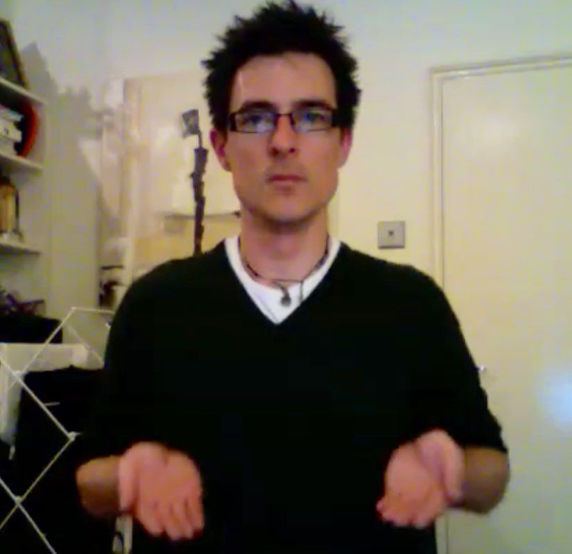
2                                                                                                   Varol, Momeni, Albanie, Afouras, Zisserman

                        “We had some pretty reasonable-sized apple trees in the garden.”      “And who knows? An apple tree might grow, or perhaps not.”

                      “What about the apple juice, you tried that? Yeah. Is it good? Yeah.”   “And who first recognised that this was such a special apple?”

    Sign: Apple
                              “A French apple tart which is cooked upside down.”                  “This is the Big Apple. This is where things are big.”

         Similarity
           score

                                                        Time frames

Fig. 1: We consider the task of sign spotting in co-articulated, continuous signing. Given a query dictionary video
of an isolated sign (e.g., “apple”), we aim to identify whether and where it appears in videos of continuous signing.
The wide domain gap between dictionary examples of isolated signs and target sequences of continuous signing
makes the task extremely challenging.

be low shot); and as one more challenge, (4) there can           Our loss formulation is an extension of InfoNCE
be multiple signs corresponding to a single keyword,         [46, 63] (and in particular the multiple instance vari-
for example due to regional variations of the sign lan-      ant MIL-NCE [41]). The novelty of our method lies
guage [50]. We show through experiments in Sec. 4, that      in the batch formulation that leverages the mouthing
directly training a sign spotter for continuous signing on   annotations, subtitles, and visual dictionaries to define
dictionary examples, obtained from an internet-sourced       positive and negative bags. Moreover, this work specif-
sign language dictionary, does indeed perform poorly.        ically focuses on computing similarities across two dif-
                                                             ferent domains to learn matching between isolated and
    To address these challenges, we propose a unified        co-articulated signing.
framework in which sign spotting embeddings are learned          We make the following contributions, originally in-
from the dictionary (to provide broad coverage of the        troduced in [43]: (1) We provide a machine readable
lexicon) in combination with two additional sources of       British Sign Language (BSL) dictionary dataset of iso-
supervision. In aggregate, these multiple types of super-    lated signs, BslDict, to facilitate study of the sign
vision include: (1) watching sign language and learning      spotting task; (2) We propose a unified Multiple In-
from existing sparse annotations obtained from mouthing stance Learning framework for learning sign embed-
cues [5]; (2) exploiting weak-supervision by reading the     dings suitable for spotting from three supervisory sources;
subtitles that accompany the footage and extracting          (3) We validate the effectiveness of our approach on a
candidates for signs that we expect to be present; (3) look- co-articulated sign spotting benchmark for which only
ing up words (for which we do not have labelled exam-        a small number (low-shot) of isolated signs are pro-
ples) in a sign language dictionary. The recent devel-       vided as labelled training examples, and (4) achieve
opment of a large-scale, subtitled dataset of continu-       state-of-the-art performance on the BSL-1K sign spot-
ous signing providing sparse annotations [5] allows us       ting benchmark [5] (closed vocabulary). We show qual-
to study this problem setting directly. We formulate         itatively that the learned embeddings can be used to
our approach as a Multiple Instance Learning prob-           (5) automatically mine new signing examples, and (6) dis-
lem in which positive samples may arise from any of          cover “faux amis” (false friends) between sign languages.
the three sources and employ Noise Contrastive Esti-         In addition, we extend these contributions with (7) the
mation [32] to learn a domain-invariant (valid across        demonstration that our framework can be effectively
both isolated and co-articulated signing) representation     deployed to obtain large numbers of sign examples, en-
of signing content.                                          abling state-of-the-art performance to be reached on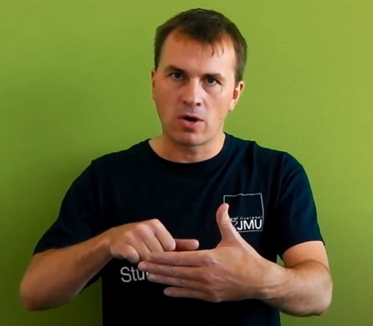
Scaling up sign spotting through sign language dictionaries                                                              3

the BSL-1K sign recognition benchmark [5], and on the       tion, since our method must bridge differences between
recently released BOBSL dataset [4].                        the dictionary and the target continuous signing dis-
                                                            tribution. A vast number of techniques have been pro-
                                                            posed to tackle distribution shift, including several ad-
2 Related Work
                                                            versarial feature alignment methods that are specialised
                                                            for the few-shot setting [44, 67]. In our work, we ex-
Our work relates to several themes in the literature: sign
                                                            plore the domain-specific batch normalization (DSBN)
language recognition (and more specifically sign spot-
                                                            method of [18], finding ultimately that simple batch
ting), sign language datasets, multiple instance learn-
                                                            normalization parameter re-initialization is instead most
ing and low-shot action localization. We discuss each of
                                                            effective when jointly training on two domains after pre-
these themes next.
                                                            training on the bigger domain. The concurrent work
Sign language recognition. The study of automatic
                                                            of [40] also seeks to align representation of isolated and
sign recognition has a rich history in the computer vi-
                                                            continuous signs. However, our work differs from theirs
sion community stretching back over 30 years, with
                                                            in several key aspects: (1) rather than assuming access
early methods developing carefully engineered features
                                                            to a large-scale labelled dataset of isolated signs, we
to model trajectories and shape [30, 37, 54, 57]. A se-
                                                            consider the setting in which only a handful of dictio-
ries of techniques then emerged which made effective
                                                            nary examples may be used to represent a word; (2)
use of hand and body pose cues through robust key-
                                                            we develop a generalised Multiple Instance Learning
point estimation encodings [10, 22, 45, 49]. Sign lan-
                                                            framework which allows the learning of representations
guage recognition also has been considered in the con-
                                                            from weakly-aligned subtitles whilst exploiting sparse
text of sequence prediction, with HMMs [3, 31, 37, 54],
                                                            labels from mouthings [5] and dictionaries (this inte-
LSTMs [11, 35, 66, 68], and Transformers [12] proving
                                                            grates cues beyond the learning formulation in [40]);
to be effective mechanisms for this task. Recently, con-
                                                            (3) we seek to label and improve performance on co-
volutional neural networks have emerged as the dom-
                                                            articulated signing (rather than improving recognition
inant approach for appearance modelling [11], and in
                                                            performance on isolated signing). Also related to our
particular, action recognition models using spatio-temporal
                                                            work, [49] uses a “reservoir” of weakly labelled sign
convolutions [16] have proven very well-suited for video-
                                                            footage to improve the performance of a sign classi-
based sign recognition [5, 36, 39]. We adopt the I3D ar-
                                                            fier learned from a small number of examples. Different
chitecture [16] as a foundational building block in our
                                                            to [49], we propose a multiple instance learning formula-
studies.
                                                            tion that explicitly accounts for signing variations that
Sign language spotting. The sign language spotting
                                                            are present in the dictionary.
problem—in which the objective is to find performances
                                                            Sign language datasets. A number of sign language
of a sign (or sign sequence) in a longer sequence of
                                                            datasets have been proposed for studying Finnish [60],
signing—has been studied with Dynamic Time Warping
                                                            German [38, 61], American [7, 36, 39, 62] and Chi-
and skin colour histograms [60] and with Hierarchical
                                                            nese [17, 35] sign recognition. For British Sign Language
Sequential Patterns [26]. Different from our work which
                                                            (BSL), [51] gathered the BSL Corpus which represents
learns representations from multiple weak supervisory
                                                            continuous signing, labelled with fine-grained linguis-
cues, these approaches consider a fully-supervised set-
                                                            tic annotations. More recently [5] collected BSL-1K,
ting with a single source of supervision and use hand-
                                                            a large-scale dataset of BSL signs that were obtained
crafted features to represent signs [27]. Our proposed
                                                            using a mouthing-based keyword spotting model. Fur-
use of a dictionary is also closely tied to one-shot/few-
                                                            ther details on this method are given in Sec. 3.1. In
shot learning, in which the learner is assumed to have
                                                            this work, we contribute BslDict, a dictionary-style
access to only a handful of annotated examples of the
                                                            dataset that is complementary to the datasets of [5, 51]
target category. One-shot dictionary learning was stud-
                                                            – it contains only a handful of instances of each sign,
ied by [49] – different to their approach, we explicitly
                                                            but achieves a comprehensive coverage of the BSL lexi-
account for variations in the dictionary for a given word
                                                            con with a 9K English vocabulary (vs a 1K vocabulary
(and validate the improvements brought by doing so in
                                                            in [5]). As we show in the sequel, this dataset enables a
Sec. 4). Textual descriptions from a dictionary of 250
                                                            number of sign spotting applications. While BslDict
signs were used to study zero-shot learning by [9] – we
                                                            does not represent a linguistic corpus, as the correspon-
instead consider the practical setting in which a handful
                                                            dences to English words and phrases are not carefully
of video examples are available per-sign and work with
                                                            annotated with glosses 2 , it is significantly larger than
a much larger vocabulary (9K words and phrases).
    The use of dictionaries to locate signs in subtitled      2
                                                                Glosses are atomic lexical units used to annotate sign lan-
video also shares commonalities with domain adapta-         guages.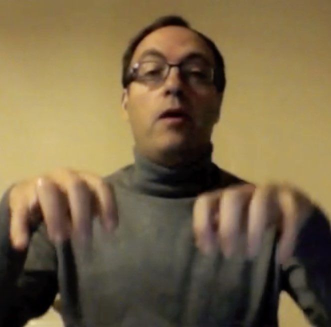
4                                                                             Varol, Momeni, Albanie, Afouras, Zisserman

                      2 - Read
                      “Oh, what it might have been is my oven was the wrong temperature.”

         1 - Watch                                           3 - Look-up

                                                              Sign: Oven

                                                             Sign: Temperature
                          Localised sign

Fig. 2: The proposed Watch, Read and Lookup framework trains sign spotting embeddings with three cues:
(1) watching videos and learning from sparse annotation in the form of localised signs obtained from mouthings [5]
(lower-left); (2) reading subtitles to find candidate signs that may appear in the source footage (top); (3) looking up
corresponding visual examples in a sign language dictionary and aligning the representation against the embedded
source segment (lower-right).

its linguistic counterparts (e.g., 4K videos correspond-     3 Learning Sign Spotting Embeddings from
ing to 2K words in BSL SignBank [29], as opposed to          Multiple Supervisors
14K videos of 9K words in BslDict), therefore Bsl-
Dict is particularly suitable to be used in conjunction      In this section, we describe the task of sign spotting and
with subtitles.                                              the three forms of supervision we assume access to. Let
                                                             XL denote the space of RGB video segments containing
                                                             a frontal-facing individual communicating in sign lan-
Multiple instance learning. Motivated by the read-           guage L and denote by XLsingle its restriction to the set of
ily available sign language footage that is accompanied      segments containing a single sign. Further, let T denote
by subtitles, a number of methods have been proposed         the space of subtitle sentences and VL = {1, . . . , V }
for learning the association between signs and words         denote the vocabulary—an index set corresponding to
that occur in the subtitle text [10, 20, 21, 49]. In this    an enumeration of written words that are equivalent to
work, we adopt the framework of Multiple Instance            signs that can be performed in L3 .
Learning (MIL) [24] to tackle this problem, previously
                                                                 Our objective, illustrated in Fig. 1, is to discover all
explored by [10, 48]. Our work differs from these works
                                                             occurrences of a given keyword in a collection of contin-
through the incorporation of a dictionary, and a princi-
                                                             uous signing sequences. To do so, we assume access to:
pled mechanism for explicitly handling sign variants, to
                                                             (i) a subtitled collection of videos containing continu-
guide the learning process. Furthermore, we generalise
                                                             ous signing, S = {(xi , si ) : i ∈ {1, . . . , I}, xi ∈ XL , si ∈
the MIL framework so that it can learn to further ex-
                                                             T }; (ii) a sparse collection of temporal sub-segments of
ploit sparse labels. We also conduct experiments at sig-
                                                             these videos that have been annotated with their cor-
nificantly greater scale to make use of the full potential
                                                             responding word, M = {(xk , vk ) : k ∈ {1, . . . , K}, vk ∈
of MIL, considering more than two orders of magnitude
                                                             VL , xk ∈ XLsingle , ∃(xi , si ) ∈ S s.t. xk ⊆ xi }; (iii) a cu-
more weakly supervised data than [10, 48].
                                                             rated dictionary of signing instances D = {(xj , vj ) : j ∈
                                                             {1, . . . , J}, xj ∈ XLsingle , vj ∈ VL }. To address the sign
Low-shot action localization. This theme investi-            spotting task, we propose to learn a data representa-
gates semantic video localization: given one or more         tion f : XL → Rd that maps video segments to vec-
query videos the objective is to localize the segment        tors such that they are discriminative for sign spotting
in an untrimmed video that corresponds semantically          and invariant to other factors of variation. Formally, for
to the query video [13, 28, 65]. Semantic matching is         3
                                                                 Sign language dictionaries provide a word-level or phrase-
too general for the sign-spotting considered in this pa-
                                                             level correspondence (between sign language and spoken lan-
per. However, we build on the temporal ordering ideas        guage) for many signs but no universally accepted glossing
explored in this theme.                                      scheme exists for transcribing languages such as BSL [56].
Scaling up sign spotting through sign language dictionaries                                                                                        5

                                Keyword Spotting Annotation Pipeline                                            Result: BSL-1K

                                                                                                                                         Happy

                                  Subs: Are you all happy with this application?

                      padding                    subtitle appears                  padding
                                     Visual keyword spotting search window
                                                                                                                                         Perfect
                     Locate occurence of target word e.g. "happy" in subtitles. Build mouthing
        Stage 1:    search window from the s second window when subtitle appears, padded by
                              p seconds on either side (to account for misalignment).
                                                                                   Happy

                                                                                                                                         Strong
       Keyword
       Spotter

                                                                                                                                        Accept

         Stage 2:   Keyword spotter locates precise 0.6 second window containing "happy" sign

Fig. 3: Mouthing-based sign annotation from [5]: (Left, the annotation pipeline): Stage 1: for a given sign
(e.g. “happy”), each instance of the word in the subtitles provides a candidate temporal segment where the sign
may occur (the subtitle timestamps are padded by several seconds to account for the asynchrony between audio-
aligned subtitles and signing interpretation); Stage 2: a mouthing visual keyword spotter uses the lip movements
of the signer to perform precise localisation of the sign within this window. (Right): Examples of localised signs
through mouthings from the BSL-1K dataset— produced by applying keyword spotting for a vocabulary of 1K
words.

any labelled pair of video segments (x, v), (x0 , v 0 ) with                               However, these temporal windows are difficult to make
x, x0 ∈ XL and v, v 0 ∈ VL , we seek a data representa-                                    use of directly since: (1) the occurrence of a keyword
tion, f , that satisfies the constraint δf (x)f (x0 ) = δvv0 ,                             in a subtitle does not ensure the presence of the corre-
where δ represents the Kronecker delta.                                                    sponding sign in the signing sequence, (2) the subtitles
                                                                                           themselves are not precisely aligned with the signing,
                                                                                           and can differ in time by several seconds. To address
3.1 Sparse annotations from mouthing cues                                                  these issues, [5] demonstrated that the sign correspond-
                                                                                           ing to a particular keyword can be localised within a
As the source of temporal video segments with corre-                                       candidate temporal window – given by the padded sub-
sponding word annotations, M, we make use of auto-                                         title timings to account for the asynchrony between the
matic annotations that were collected as part of our                                       audio-aligned subtitles and signing interpretation – by
prior work on visual keyword spotting with mouthing                                        searching for its spoken components [56] amongst the
cues [5], which we briefly recap here. Signers sometimes                                   mouth movements of the interpreter. While there are
mouth a word while simultaneously signing it, as an                                        challenges associated with using spoken components as
additional signal [8, 55, 56], performing similar lip pat-                                 a cue (signers do not typically mouth continuously and
terns as for the spoken word. Fig. 3 presents an overview                                  may only produce mouthing patterns that correspond
of how we use such mouthings to spot signs.                                                to a portion of the keyword [56]), it has the significant
    As a starting point for this approach, we assume                                       advantage of transforming the general annotation prob-
access to TV footage that is accompanied by: (i) a                                         lem from classification (i.e., “which sign is this?”) into
frontal facing sign language interpreter, who provides                                     the much easier problem of localisation (i.e., “find a
a translation of the spoken content of the video, and                                      given token amongst a short sequence”). In [5], the vi-
(ii) a subtitle track, representing a direct transcription                                 sual keyword spotter uses the candidate temporal win-
of the spoken content. The method of [5] first searches                                    dow with the target keyword to estimate the probabil-
among the subtitles for any occurrences of “keywords”                                      ity that the sign was mouthed at each time step. If the
from a given vocabulary. Subtitles containing these key-                                   peak probability over time is above a threshold param-
words provide a set of candidate temporal windows in                                       eter, the predicted location of the sign is taken as the
which the interpreter may have produced the sign cor-                                      0.6 second window starting before the position of the
responding to the keyword (see Fig. 3, Left, Stage 1).
6                                                                           Varol, Momeni, Albanie, Afouras, Zisserman

peak probability (see Fig. 3, Left, Stage 2). For building   To incorporate the available sources of supervision into
the BSL-1K dataset, [5] uses a probability threshold of      this formulation, we consider two categories of positive
0.5 and runs the visual keyword spotter with a vocab-        and negative bag formations, described next (a formal
ulary of 1,350 keywords across 1,000 hours of signing.       mathematical description of the positive and negative
A further filtering step is performed on the vocabu-         bags described below is deferred to Appendix C.2).
lary to ensure that each word included in the dataset is     Watch and Lookup: using sparse annotations and
represented with high confidence (at least one instance      dictionaries. Here, we describe a baseline where we
with confidence 0.8) in the training partition, which        assume no subtitles are available. To learn f from M
produces a final dataset vocabulary of 1,064 words. The      and D, we define each positive bag as the set of possible
resulting BSL-1K dataset has 273K mouthing annota-           pairs between a labelled (foreground ) temporal segment
tions, some of which are illustrated in Fig. 3 (right). We   of a continuous video from M and the examples of the
employ these annotations directly to form the set M in       corresponding sign in the dictionary (green regions in
this work.                                                   Fig A.2). The key assumption here is that each labelled
                                                             sign segment from M matches at least one sign varia-
                                                             tion in the dictionary. Negative bags are constructed by
3.2 Integrating cues through multiple instance learning
                                                             (i) anchoring on a continuous foreground segment and
To learn f , we must address several challenges. First, as   selecting dictionary examples corresponding to differ-
noted in Sec. 1, there may be a considerable distribu-       ent words from other batch items; (ii) anchoring on a
tion shift between the dictionary videos of isolated signs   dictionary foreground set and selecting continuous fore-
in D and the co-articulated signing videos in S. Second,     ground segments from other batch items (red regions in
sign languages often contain multiple sign variants for      Fig A.2). To maximize the number of negatives within
a single written word (e.g., resulting from regional vari-   one minibatch, we sample a different word per batch
ations and synonyms). Third, since the subtitles in S        item.
are only weakly aligned with the sign sequence, we must      Watch, Read and Lookup: using sparse anno-
learn to associate signs and words from a noisy signal       tations, subtitles and dictionaries. Using just the
that lacks temporal localisation. Fourth, the localised      labelled sign segments from M to construct bags has a
annotations provided by M are sparse, and therefore          significant limitation: f is not encouraged to represent
we must make good use of the remaining segments of           signs beyond the initial vocabulary represented in M.
subtitled videos in S if we are to learn an effective rep-   We therefore look at the subtitles (which contain words
resentation.                                                 beyond M) to construct additional bags. We determine
    Given full supervision, we could simply adopt a pair-    more positive bags between the set of unlabelled (back-
wise metric learning approach to align segments from         ground) segments in the continuous footage and the set
the videos in S with dictionary videos from D by requir-     of dictionaries corresponding to the background words
ing that f maps a pair of isolated and co-articulated        in the subtitle (green regions in Fig. 4, right-bottom).
signing segments to the same point in the embedding          Negatives (red regions in Fig. 4) are formed as the com-
space if they correspond to the same sign (positive pairs)   plements to these sets by (i) pairing continuous back-
and apart if they do not (negative pairs). As noted          ground segments with dictionary samples that can be
above, in practice we do not have access to positive pairs   excluded as matches (through subtitles) and (ii) pair-
because: (1) for any annotated segment (xk , vk ) ∈ M,       ing background dictionary entries with the foreground
we have a set of potential sign variations represented in    continuous segment. In both cases, we also define neg-
the dictionary (annotated with the common label vk ),        atives from other batch items by selecting pairs where
rather than a single unique sign; (2) since S provides       the word(s) have no overlap, e.g., in Fig. 4, the dictio-
only weak supervision, even when a word is mentioned         nary examples for the background word ‘speak’ from
in the subtitles we do not know where it appears in          the second batch item are negatives for the background
the continuous signing sequence (if it appears at all).      continuous segments from the first batch item, corre-
These ambiguities motivate a Multiple Instance Learn-        sponding to the unlabelled words ‘name’ and ‘what’ in
ing [24] (MIL) objective. Rather than forming positive       the subtitle.
and negative pairs, we instead form positive bags of             To assess the similarity of two embedded video seg-
pairs, P bags , in which we expect at least one pairing      ments, we employ a similarity function ψ : Rd ×Rd → R
between a segment from a video in S and a dictionary         whose value increases as its arguments become more
video from D to contain the same sign, and negative          similar (in this work, we use cosine similarity). For no-
bags of pairs, N bags , in which we expect no (video seg-    tational convenience below, we write ψij as shorthand
ment, dictionary video) pair to contain the same sign.       for ψ(f (xi ), f (xj )). To learn f , we consider a general-
Scaling up sign spotting through sign language dictionaries                                                                                                                                     7

              friend                        friend                      name          what
  batch

           language                        language                             speak
                                                                                                             Continuous foreground                           Dictionary foreground
          }

                                     foreground word                    background words

          Continuous signing                         Dictionary exemplars                                    Continuous background                          Dictionary background

Fig. 4: Batch sampling and positive/negative pairs: We illustrate the formation of a batch when jointly
training on continuous signing video (squares) and dictionaries of isolated signing (circles). Left: For each contin-
uous video, we sample the dictionaries corresponding to the labelled word (foreground), as well as to the rest of
the subtitles (background). Right: We construct positive/negative pairs by anchoring at 4 different portions of
a batch item: continuous foreground/background and dictionary foreground/background. Positives and negatives
(defined across continuous and dictionary domains) are green and red, respectively; anchors have a dashed border
(see Appendix C.2 for details).

ization of the InfoNCE loss [46, 63] (a non-parametric                                           Since we find that dictionary videos of isolated signs
softmax loss formulation         of Noise Contrastive Estima-                                    tend to be performed more slowly, we uniformly sam-
                       Figure: Batch sampling and positive/negative pairs: We illustrate the formation of a batch when jointly training on BSL-1K continuous video and
                       BSL-Dict isolated dictionary videos. Top: For each continuous video, we sample the dictionaries corresponding to the labeled word (foreground), as well as
tion [32]) recently proposed           by     [41]   as    MIL-NCE               loss:           ple 16 frames from each dictionary video with a random
                       the dictionaries corresponding to the subtitles (background). Bottom: We construct positive/negative pairs by anchoring at 4 different portions of a batch
                       item: BSL-1K foreground/background and BSL-Dict foreground/background.      The anchor
                                                                                                 shift    andis denoted
                                                                                                                   random  with lightframe
                                                                                                                                      green, positives
                                                                                                                                                 ratefromnthetimes,
                                                                                                                                                                other domain  as dark n is propor-
                                                                                                                                                                           where
                       green, negatives from the other domain as red. We mark the orange samples as negatives if there is no overlap within subtitles or word labels, otherwise we
                       discard them.  Note that we sample a 1 BSL-1K foreground sample per wordtional
                                                                                                  in an entireto
                                                                                                               batchthe     length
                                                                                                                     to maximize           of
                                                                                                                                   the number  ofthe     video,
                                                                                                                                                  negatives.           and     pass these clips
                                               eψjk /τ
                                   P
          "                                                                   #
                             (j,k)∈P(i)                                                          through          the     I3D       trunk        then      average          the     resulting vec-
L = −Ei log                                                                      ,   (1)         tors    before         they       are    processed            by     the    MLP       to produce
                            eψjk /τ +
                    P                               P
                                                                eψlm /τ
                (j,k)∈P(i)                    (l,m)∈N (i)                                        the final dictionary embeddings. We find that this form
                                                                                                 of random sampling performs better than sampling 16
    where P(i) ∈ P bags , N (i) ∈ N bags , τ , often referred                                    consecutive frames from the isolated signing videos (see
to as the temperature, is set as a hyperparameter (we                                            Appendix C.1 for more details). During pretraining,
explore the effect of its value in Sec. 4).                                                      minibatches of size 4 are used; and colour, scale and
                                                                                                 horizontal flip augmentations are applied to the input
                                                                                                 video, following the procedure described in [5]. The
3.3 Implementation details
                                                                                                 trunk parameters are then frozen and the MLP outputs
                                                                                                 are used as embeddings. Both datasets are described in
In this section, we provide details for the learning frame-
                                                                                                 detail in Sec. 4.1.
work covering the embedding architecture, sampling
protocol and optimization procedure.                                                             Minibatch sampling. To train the MLP given the
Embedding architecture. The architecture comprises pretrained I3D features, we sample data by first iter-
an I3D spatio-temporal trunk network [16] to which we                                            ating over the set of labelled segments comprising the
attach an MLP consisting of three linear layers sepa-                                            sparse annotations, M, that accompany the dataset of
rated by leaky ReLU activations (with negative slope                                             continuous, subtitled sampling to form minibatches. For
0.2) and a skip connection. The trunk network takes as                                           each continuous video, we sample 16 consecutive frames
input 16 frames from a 224 × 224 resolution video clip                                           around the annotated timestamp (more precisely a ran-
and produces 1024-dimensional embeddings which are                                               dom offset within 20 frames before, 5 frames after, fol-
then projected to 256-dimensional sign spotting embed-                                           lowing the timing study in [5]). We randomly sample 10
dings by the MLP. More details about the embedding                                               additional 16-frame clips from this video outside of the
architecture can be found in Appendix C.1.                                                       labelled window, i.e., continuous background segments.
Joint pretraining. The I3D trunk parameters are ini-                                             For each subtitled sequence, we sample the dictionary
tialised by pretraining for sign classification jointly over                                     entries for all subtitle words that appear in VL (see
the sparse annotations M of a continuous signing dataset Fig. 4 for a sample batch formation).
(BSL-1K [5]) and examples from a sign dictionary dataset                                               Our minibatch comprises 128 sequences of continu-
(BslDict) which fall within their common vocabulary.                                                ous signing and their corresponding dictionary entries
8                                                                            Varol, Momeni, Albanie, Afouras, Zisserman

(we investigate the impact of batch size in Sec. 4.4).        4.1 Datasets
The embeddings are then trained by minimising the loss
defined in Eqn.(1) in conjunction with positive bags,         Although our method is conceptually applicable to a
P bags , and negative bags, N bags , which are constructed    number of sign languages, in this work we focus primar-
on-the-fly for each minibatch (see Fig. 4).                   ily on BSL, the sign language of British deaf commu-
Optimization. We use a SGD optimizer with an initial          nities. We use BSL-1K [5], a large-scale, subtitled and
learning rate of 10−2 to train the embedding architec-        sparsely annotated dataset of more than 1,000 hours
ture. The learning rate is decayed twice by a factor of       of continuous signing which offers an ideal setting in
10 (at epochs 40 and 45). We train all models, including      which to evaluate the effectiveness of the Watch, Read
baselines and ablation studies, for 50 epochs at which        and Lookup sign spotting framework. To provide dictio-
point we find that learning has always converged.             nary data for the lookup component of our approach,
Test time. To perform spotting, we obtain the embed-          we also contribute BslDict, a diverse visual dictionary
dings learned with the MLP. For the dictionary, we have       of signs. These two datasets are summarised in Tab. 1
a single embedding averaged over the video. Continu-          and described in more detail below. We further include
ous video embeddings are obtained with sliding window         experiments on a new dataset, BOBSL [4], which we
(stride 1) on the entire sequence. We show the impor-         describe in Sec. 4.7 together with results. The BOBSL
tance of using such a dense stride for a precise localisa-    dataset has similar properties to BSL-1K.
tion in our ablations (Sec. 4.4). However, for simplicity,    BSL-1K [5] comprises over 1,000 hours of video of
all qualitative visualisations are performed with contin-     continuous sign-language-interpreted television broad-
uous video embeddings obtained with a sliding window          casts, with accompanying subtitles of the audio content.
of stride 8.                                                  In [5], this data is processed for the task of individual
    We calculate the cosine similarity score between the      sign recognition: a visual keyword spotter is applied
continuous signing sequence embeddings and the em-            to signer mouthings giving a total of 273K sparsely
bedding for a given dictionary video. We determine the        localised sign annotations from a vocabulary of 1,064
location with the maximum similarity as the location          signs (169K in the training partition as shown in Tab. 1).
of the queried sign. We maintain embedding sets of            Please refer to Sec. 3.1 and [5] for more details on the
all variants of dictionary videos for a given word and        automatic annotation pipeline. We refer to Sec. 4.6 for a
choose the best match as the one with the highest sim-        description of the BSL-1K sign recognition benchmark
ilarity.                                                      (TestRec            Rec
                                                                    2K and Test37K in Tab. 1).
                                                                  In this work, we process this data for the task of
                                                              retrieval, extracting long videos with associated subti-
                                                              tles. In particular, we pad ±2 seconds around the sub-
4 Experiments                                                 title timestamps and we add the corresponding video
                                                              to our training set if there is a sparse annotation from
In this section, we first present the datasets used in this   mouthing falling within this time window – we assume
work (including the contributed BslDict dataset) in           this constraint indicates that the signing is reasonably
Sec. 4.1, followed by the evaluation protocol in Sec. 4.2.    well-aligned with its subtitles. We further consider only
We then illustrate the benefits of the Watch, Read and        the videos whose subtitle duration is longer than 2 sec-
Lookup learning framework for sign spotting against           onds. For testing, we use the automatic test set (corre-
several baselines (Sec. 4.3) with a comprehensive abla-       sponding to mouthing locations with confidences above
tion study that validates our design choices (Sec. 4.4).      0.9). Thus we obtain 78K training (TrainReT ) and 2K
Next, we investigate three applications of our method in      test (TestReT ) videos as shown in Tab. 1, each of which
Sec. 4.5, showing that it can be used to (i) not only spot    has a subtitle of 8 words on average and 1 sparse mouthing
signs, but also identify the specific sign variant that       annotation.
was used, (ii) label sign instances in continuous signing
footage given the associated subtitles, and (iii) discover    BslDict. BSL dictionary videos are collected from a
“faux amis” between different sign languages. We then         BSL sign aggregation platform signbsl.com [1], giving
provide experiments on sign language recognition, sig-        us a total of 14,210 video clips for a vocabulary of 9,283
nificantly improving the state of the art by applying         signs. Each sign is typically performed several times by
our labelling technique to obtain more training exam-         different signers, often in different ways. The dictionary
ples automatically (Sec. 4.6 and Sec. 4.7). Finally, we       videos are linked from 28 known website sources and
discuss limitations of our sign spotting technique using      each source has at least 1 signer. We used face embed-
dictionaries (Sec. 4.8).                                      dings computed with SENet-50 [34] (trained on VG-
Scaling up sign spotting through sign language dictionaries                                                                  9

   Dataset     Split        #Videos     Vocabulary    #Signers                            Examples
               TrainRec        169K           1,064            36
               TestRec
                   2K          2,103            334             4
               TestRec
                   37K        36,854            950             4
  BSL-1K[5]
               TrainReT       78,211          1,064            36
               TestReT         1,834            264             4

  BslDict      Full           14,210          9,283           124
               1K-subset       2,963          1,064            70

Table 1: Datasets: We provide (i) the number of individual signing videos, (ii) the vocabulary size of the annotated
signs, and (iii) the number of signers for several subsets of BSL-1K and BslDict. BSL-1K is large in the number
of annotated signs whereas BslDict is large in the vocabulary size. Note that BSL-1K is constructed differently
depending on whether it is used for the task of recognition or retrieval: for retrieval, longer signing sequences are
used around individual localised signs as described in Sec. 4.1.

GFace2 [14]) to cluster signer identities and manually              Metrics. The performance is evaluated based on rank-
verified that there are a total of 124 different signers.           ing metrics as in retrieval. For every sign si in the test
The dictionary videos are of isolated signs (as opposed             vocabulary, we first select the BSL-1K test set clips
to co-articulated in BSL-1K): this means (i) the start              which have a mouthing annotation of si and then record
and end of the video clips usually consist of a still signer        the percentage of times that a dictionary clip of si ap-
pausing, and (ii) the sign is performed at a much slower            pears in the first 5 retrieved results, this is the ‘Recall
rate for clarity. We first trim the sign dictionary videos,         at 5’ (R@5). This is motivated by the fact that different
using body keypoints estimated with OpenPose [15]                   English words can correspond to the same sign, and vice
which indicate the start and end of wrist motion, to                versa. We also report mean average precision (mAP).
discard frames where the signer is still. With this pro-            For each video pair, the match is considered correct if
cess, the average number of frames per video drops from             (i) the dictionary clip corresponds to si and the BSL-1K
78 to 56 (still significantly larger than co-articulated            video clip has a mouthing annotation of si , and (ii) if
signs). To the best of our knowledge, BslDict is the                the predicted location of the sign in the BSL-1K video
first curated, BSL sign dictionary dataset for computer             clip, i.e., the time frame where the maximum similar-
vision research. A collection of metadata associated for            ity occurs, lies within certain frames around the ground
the BslDict dataset is made publicly available, as well             truth mouthing timing. In particular, we determine the
as our pre-computed video embeddings from this work.                correct interval to be defined between 20 frames before
    For the experiments in which BslDict is filtered                and 5 frames after the labelled time (based on the study
to the 1,064 vocabulary of BSL-1K, we have 3K videos                in [5]). Finally, because the BSL-1K test set is class-
as shown in Tab. 1. Within this subset, each sign has               unbalanced, we report performances averaged over the
between 1 and 10 examples (average of 3).                           test classes.

4.2 Evaluation protocols                                            4.3 Comparison to baselines

Protocols. We define two settings: (i) training with                In this section, we evaluate different components of our
the entire 1,064 vocabulary of annotations in BSL-1K;               approach. We first compare our contrastive learning ap-
and (ii) training on a subset with 800 signs. The latter            proach with classification baselines. Then, we investi-
is needed to assess the performance on novel signs, for             gate the effect of our multiple-instance loss formula-
which we do not have access to co-articulated labels at             tion. Finally, we report performance on a sign spotting
training. We thus use the remaining 264 words for test-             benchmark.
ing. This test set is therefore common to both training             I3D baselines. We start by evaluating baseline I3D
settings, it is either ‘seen’ or ‘unseen’ at training. How-         models trained with classification on the task of spot-
ever, we do not limit the vocabulary of the dictionary              ting, using the embeddings before the classification layer.
as a practical assumption, for which we show benefits.              We have three variants in Tab. 2: (i) I3DBSL-1K pro-
10                                                                                 Varol, Momeni, Albanie, Afouras, Zisserman

                                                                  Train (1064)                               Train (800)
                                                                   Seen (264)                                Unseen (264)
     Embedding arch.           Supervision             mAP                R@5                   mAP                  R@5
     I3DBslDict                Classification           2.68                 3.57                1.21                  1.29
     I3DBSL-1K [5]             Classification          13.09                17.25                6.74                  8.94
     I3DBSL-1K,BslDict         Classification          19.81                25.57                4.81                  6.89
     I3DBSL-1K,BslDict +MLP    Classification          37.13 ± 0.29         39.68 ± 0.57        10.33 ± 0.43          13.33 ± 1.11
     I3DBSL-1K,BslDict +MLP    InfoNCE                 43.59 ± 0.76         52.59 ± 0.75        11.40 ± 0.42          14.76 ± 0.40
     I3DBSL-1K,BslDict +MLP    Watch-Lookup            44.72 ± 0.85         55.51 ± 2.17        11.02 ± 0.27          15.03 ± 0.45
     I3DBSL-1K,BslDict +MLP    Watch-Read-Lookup       47.93 ± 0.20         60.76 ± 1.45        14.86 ± 1.29          19.85 ± 1.94

Table 2: The effect of the loss formulation: Embeddings learned with the classification loss are suboptimal
since they are not trained for matching the two domains. Contrastive-based loss formulations (NCE) significantly
improve, particularly when we adopt the multiple-instance variant introduced as our Watch-Read-Lookup frame-
work of multiple supervisory signals. We report the relatively cheaper MLP-based models with three random seeds
for each model and report the mean and the standard deviation.

vided by [5] which is trained only on the BSL-1K dataset,           Supervision         Dictionary Vocab        mAP            R@5

and we also train (ii) I3DBslDict and (iii) I3DBSL-1K,BslDict .     Watch-Read-Lookup
                                                                    Watch-Read-Lookup
                                                                                        800 training vocab
                                                                                        9k full vocab
                                                                                                             14.86 ± 1.29
                                                                                                             15.82 ± 0.48
                                                                                                                            19.85 ± 1.94
                                                                                                                            21.67 ± 0.72
Training only on BslDict (I3DBslDict ) performs sig-
nificantly worse due to the few examples available per            Table 3: Extending the dictionary vocabulary: We
class and the domain gap that must be bridged to spot             show the benefits of sampling dictionary videos outside
co-articulated signs, suggesting that dictionary samples          of the sparse annotations, using subtitles. Extending
alone do not suffice to solve the task. We observe im-            the lookup to the dictionary from the subtitles to the
provements with fine-tuning I3DBSL-1K jointly on the              full vocabulary of BslDict brings significant improve-
two datasets (I3DBSL-1K,BslDict ), which becomes our              ments for novel signs (the training uses sparse anno-
base feature extractor for the remaining experiments              tations for the 800 words, and the remaining 264 for
to train a shallow MLP.                                           test).

Loss formulation. We first train the MLP parameters
on top of the frozen I3D trunk with classification to es-         using the full 9k vocabulary from BslDict improves
tablish a baseline in a comparable setup. Note that, this         the results on the unseen setting.
shallow architecture can be trained with larger batches           BSL-1K sign spotting benchmark. Although our
than I3D. Next, we investigate variants of our loss to            learning framework primarily targets good performance
learn a joint sign embedding between BSL-1K and Bsl-              on unseen continuous signs, it can also be naively ap-
Dict video domains: (i) standard single-instance In-              plied to the (closed-vocabulary) sign spotting bench-
foNCE [46, 63] loss which pairs each BSL-1K video clip            mark proposed by [5]. The sign spotting benchmark
with one positive BslDict clip of the same sign, (ii)             requires a model to localise every instance belonging to
Watch-Lookup which considers multiple positive dictio-            a given set of sign classes (334 in total) within long se-
nary candidates, but does not consider subtitles (there-          quences of untrimmed footage. The benchmark is chal-
fore limited to the annotated video clips). Tab. 2 sum-           lenging because each sign appears infrequently (cor-
marises the results. Our Watch-Read-Lookup formula-               responding to approximately one positive instance in
tion which effectively combines multiple sources of su-           every 90 minutes of continuous signing). We evaluate
pervision in a multiple-instance framework outperforms            the performance of our Watch-Read-Lookup model and
the other baselines in both seen and unseen protocols.            achieve a score of 0.170 mAP, outperforming the previ-
                                                                  ous state-of-the-art performance of 0.160 mAP [5].
Extending the vocabulary. The results presented so
far were using the same vocabulary for both continu-
ous and dictionary datasets. In reality, one can assume
access to the entire vocabulary in the dictionary, but            4.4 Ablation study
obtaining annotations for the continuous videos is pro-
hibitive. Tab. 3 investigates removing the vocabulary             We provide ablations for the learning hyperparame-
limit on the dictionary side, but keeping the continu-            ters, such as the batch size and the temperature; the
ous annotations vocabulary at 800 signs. We show that             mouthing confidence threshold as the training data se-
Scaling up sign spotting through sign language dictionaries 11
(a) (b)
Fig. 5: The effect of (a) the batch size that determines the number of negatives across sign classes and (b) the
temperature hyper-parameter for the MIL-NCE loss in Watch-Lookup against mAP and R@5 (trained on the
full 1064 vocab.)
lection parameter; and the stride parameter of the slid- Mouthing confidence Training size mAP R@5
ing window at test time. 0.9 10K 37.55 47.54
Batch size. Next, we investigate the effect of increas- 0.8 21K 39.49 48.84
0.7 33K 41.87 51.15
ing the number of negative pairs by increasing the batch 0.6 49K 42.44 52.42
size when training with Watch-Lookup on 1,064 cate- 0.5 78K 43.65 53.03
gories. We observe in Fig. 5(a) an improvement in per-
formance with a greater number of negatives before sat- Table 4: Mouthing confidence threshold: The re-
urating. Our final Watch-Read-Lookup model has high sults suggest that lower confidence automatic annota-
memory requirements, for which we use 128 batch size. tions of BSL-1K provide better training, by increasing
Note that the effective size of the batch with our sam- the amount of data (training on the full 1064 vocabu-
pling is larger due to sampling extra video clips corre- lary with Watch-Lookup).
sponding to subtitles.
Temperature. Finally, we analyze the impact of the
we investigate the effect of the stride parameter. Our
temperature hyperparameter τ on the performance of
window size is 16 frames, i.e., the number of input
Watch-Lookup. We conclude from Fig. 5(b) that set-
frames for the I3D feature extractor. A standard ap-
ting τ to values between [0.04 - 0.10] does not im-
proach when extracting features from longer videos is
pact the performance significantly; therefore, we keep
to use a sliding window with 50% overlap (i.e., stride
τ = 0.07 following the previous work [33, 63] for all
of 8 frames). However, this means the temporal reso-
other experiments. However, values outside this range
lution of the search space is reduced by a factor of 8,
negatively impact the performance, especially for high
and a stride of 8 may skip the most discriminative mo-
values, i.e., {0.50, 1.00}; we observe a major decrease in
ment since a sign duration is typically between 7-13
performance when τ approaches 1.
frames (but can be shorter) [48] in continuous signing
Mouthing confidence threshold at training. As video. In Tab. 5, we see that we can gain a significant
explained in Sec. 3.1, the sparse annotations from the localisation improvement by computing the similarities
BSL-1K dataset are obtained automatically by running more densely, e.g., stride of 4 frames may be sufficiently
a visual keyword spotting method based on mouthing dense. In our experiments, we use stride 1.
cues. The dataset provides a confidence value associ- We refer to Appendix B for additional ablations.
ated with each label ranging between 0.5 and 1.0. Sim-
ilar to [5], we experiment with different thresholds to
determine the training set. Lower thresholds result in 4.5 Applications
a noisier but larger training set. From Tab. 4, we con-
clude that 0.5 mouthing confidence threshold performs In this section, we investigate three applications of our
the best. This is in accordance with the conclusion from sign spotting method.
[5]. Sign variant identification. We show the ability of
Effect of the sliding window stride. As explained our model to spot specifically which variant of the sign
in Sec. 3.3, at test time, we extract features from the was used. In Fig. 6, we observe high similarity scores
continuous signing sequence using a sliding window ap- when the variant of the sign matches in both BSL-1K
proach with 1 frame as the stride parameter. In Tab. 5, and BslDict videos. Identifying such sign variations12 Varol, Momeni, Albanie, Afouras, Zisserman
Similarity score “One of Britain’s worst cases of animal cruelty.” “I’ve never known you talk like this before, Johnnie. It’s mad!”
Sign: Animal Sign: Before
Time frames
Fig. 6: Sign variant identification: We plot the similarity scores between BSL-1K test clips and BslDict
variants of the sign “animal” (left) and “before” (right) over time. A high similarity occurs for the first two rows,
where the BslDict examples match the variant used in BSL-1K. The labelled mouthing times from [5] are shown
by red vertical lines and approximate windows for signing times are shaded. Note that neither the mouthing
annotations (ground truth) nor the dictionary spottings provide the duration of the sign, but only a point in time
where the response is highest. The mouthing peak (red vertical line) tends to appear at the end of the sign (due
to the use of LSTM in visual keyword spotter). The dictionary peak (blue curve) tends to appear in the middle of
the sign.
“The only thing that’s wrong here, Sir, is the weather.” “It is a huge project, we are bringing 4.5 million tonnes.”
Sign: Only Sign: Project
Similarity score
Sign: Wrong Sign: Bring
Sign: Weather Sign: Million
Time frames
Fig. 7: Densification: We plot the similarity scores between BSL-1K test clips and BslDict examples over time,
by querying only the words in the subtitle. We visually inspect the quality of the dictionary spottings with which
we obtain cases of multiple words per subtitle spotted. The predicted locations of the signs correspond to the peak
similarity scores. Note that unlike in Fig. 6, we cannot overlay the ground truth since the annotations using the
mouthing cues are not dense enough to provide ground truth sign locations for 3 words per subtitle.
allows a better understanding of regional differences els. In Fig. 7, we show qualitative examples of localising
and can potentially help standardisation efforts of BSL. multiple signs in a given sentence in BSL-1K, where we
Dense annotations. We demonstrate the potential of only query the words that occur in the subtitles, reduc-
our model to obtain dense annotations on continuous ing the search space. In fact, if we assume the word to
sign language video data. Sign spotting through the be known, we obtain 83.08% sign localisation accuracy
use of sign dictionaries is not limited to mouthings as on BSL-1K with our best model. This is defined as the
in [5] and therefore is of great importance to scale up number of times the maximum similarity occurs within
datasets for learning more robust sign language mod- -20/+5 frames of the end label time provided by [5].Scaling up sign spotting through sign language dictionaries 13
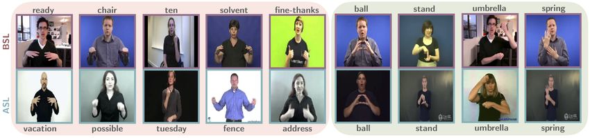
Fig. 8: “Faux amis” in BSL/ASL: Same/similar manual features for different English words (left), as well as
for the same English words (right), are identified between BslDict and WLASL isolated sign language datasets.
Stride mAP R@5 new localised sign instances. This allows us to train a
sign recognition model: in this case, to retrain the I3D
16 31.96 38.98
architecture from [5] which was previously supervised
8 38.46 47.38
4 44.92 54.65 only with signs localised through mouthings.
2 45.39 55.63
1 43.65 53.03 BSL-1K automatic annotation. Similar to our pre-
vious work using mouthing cues [5], where words in
Table 5: Stride parameter of sliding window: A the subtitle were queried within a neighborhood around
small stride at test time, when extracting embeddings the subtitle timestamps, we query each subtitle word
from the continuous signing video, allows us to tempo- if they fall within a predefined set of vocabulary. In
rally localise the signs more precisely. The window size particular, we query words and phrases from the 9K
is 16 frames and the typical co-articulated sign dura- BslDict vocabulary if they occur in the subtitles. To
tion is 7-13 frames at 25 fps. (testing 1064-class model determine whether a query from the dictionary occurs
trained with Watch-Lookup) in the subtitle, we apply several checks. We look for
the original word or phrase as it appears in the dic-
tionary, as well as its text-normalised form (e.g., “20”
“Faux Amis”. There are works investigating lexical becomes “twenty”). For the subtitle, we look for its orig-
similarities between sign languages manually [6, 52]. inal, text-normalised, and lemmatised forms. Once we
We show qualitatively the potential of our model to find a match between any form of the dictionary text
discover similarities, as well as “faux-amis” between and any form of the subtitle text, we query the dic-
different sign languages, in particular between British tionary video feature within the search window in the
(BSL) and American (ASL) Sign Languages. We re- continuous video features. We use search windows of ±4
trieve nearest neighbors according to visual embedding seconds padding around the subtitle timestamps. We
similarities between BslDict which has a 9K vocabu- compute the similarity between the continuous signing
lary and WLASL [39], an ASL isolated sign language search window and each of the dictionary variants for a
dataset with a 2K vocabulary. We provide some exam- given word: we record the frame location of maximum
ples in Fig. 8. We automatically identify several signs similarity for all variants and choose the best match
with similar manual features some of which correspond as the one with highest similarity score. The final sign
to different meanings in English (left), as well as same localisations are obtained by filtering the peak simi-
meanings, such as “ball”, “stand”, “umbrella” (right). larity scores to those above 0.7 threshold – resulting
in a vocabulary of 4K signs – and taking 32 frames
centered around the peak location. Fig. 9 summarises
4.6 Sign language recognition several statistics computed over the training set. We
note that sign spotting with dictionaries (D) is more
As demonstrated qualitatively in Sec. 4.5, we can reli- effective than with mouthing (M) in terms of the yield
ably obtain automatic annotations using our sign spot- (510K versus 169K localised signs). Since, D can in-
ting technique when the search space is reduced to can- clude duplicates from M, we further report the number
didate words in the subtitle. A natural way to exploit of instances for which a mouthing spotting for the same
our method is to apply it on the BSL-1K training set in keyword query exists within the same search window.
conjunction with the weakly-aligned subtitles to collect We find that the majority of our D spottings repre-14 Varol, Momeni, Albanie, Afouras, Zisserman
Yield for 1K query vocabulary Yield for 9K query vocabulary
Fig. 9: Statistics on the yield from the automatic annotations: We plot the vocabulary size (left) and the
number of localised sign instances (middle) and (right) over several similarity thresholds for the new automatic
annotations in the training set that we obtain through dictionaries. While we obtain a large number of localised
signs (783K at 0.7 threshold) for the full 9K vocabulary, in our recognition experiments we use a subset of 510K
annotations that correspond to the 1K vocabulary. To approximately quantify the amount of annotations that
represent duplicates from those found through mouthing cues, we count those localisations for which the same
keyword exists for mouthing annotations within the same search window. We observe that the majority of the
annotations are new (783K vs 122K).
sent new, not previously localised instances (see Fig. 9 TestRec
2K [5] TestRec
37K
right). 2K inst. / 334 cls. 37K inst. / 950 cls.
BSL-1K sign recognition benchmark. We use the per-instance per-class per-instance per-class
BSL-1K manually verified recognition test set with 2K Training #ann. top-1 top-5 top-1 top-5 top-1 top-5 top-1 top-5
samples [5], which we denote with TestRec 2K , and signifi-
M [5]§ 169K 76.6 89.2 54.6 71.8 26.4 41.3 19.4 33.2
D 510K 70.8 84.9 52.7 68.1 60.9 80.3 34.7 53.5
cantly extend it to 37K samples as TestRec 37K . We do this M+D 678K 80.8 92.1 60.5 79.9 62.3 81.3 40.2 60.1
by (a) running our dictionary-based sign spotting tech-
nique on the BSL-1K test set and (b) verifying the pre-
Table 6: An improved I3D sign recognition
dicted sign instances with human annotators using the
model: We find signs via automatic dictionary spot-
VIA tool [25] as in [5]. Our goal in keeping these two di-
ting (D), significantly expanding the training and test-
visions is three-fold: (i) TestRec
2K is the result of annotat- ing data obtained from mouthing cues by [5] (M). We
ing “mouthing” spottings above 0.9 confidence, which
also significantly expand the test set by manually ver-
means the models can largely rely on mouthing cues to
ifying these new automatic annotations from the test
recognise the signs. The new TestRec 37K annotations have partition (TestRec Rec
2K vs Test37K ). By training on the ex-
both “mouthing” (10K) and “dictionary” (27K) spot-
tended M+D data, we obtain state-of-the-art results,
tings. The dictionary annotations are the result of an-
outperforming the previous work of [5]. §The slight im-
notating dictionary spottings above 0.7 confidence from
provement in the performance of [5] over the original
this work; therefore, models are required to recognise
results reported in that work is due to our denser test-
the signs even in the absence of mouthing, reducing the
time averaging when applying sliding windows (8-frame
bias towards signs with easily spotted mouthing cues.
vs 1-frame stride).
(ii) TestRec
37K spans a much larger fraction of the training
vocabulary as seen in Tab. 1, with 950 out of 1,064 sign
classes (vs only 334 classes in the original benchmark
TestRec
2K of [5]). (iii) We wish to maintain direct com- vs 76.6%). This may be due to the strong bias towards
parison to our previous work [5]; therefore, we report mouthing cues in the small test set TestRec 2K . Second,
on both sets in this work. the benefits of combining annotations from both can
Comparison to prior work. In Tab. 6, we compare be seen in the sign classifier trained using 678K auto-
three I3D models trained on mouthing annotations (M), matic annotations. This obtains state-of-the-art perfor-
dictionary annotations (D) , and their combination (M+D). mance on TestRec 2K , as well as the more challenging test
First, we observe that D-only model significantly out- set TestRec
37K . All three models in the table (M, D, M+D)
Rec
performs M-only model on Test37K (60.9% vs 26.4%), are pretrained on Kinetics [16], followed by video pose
while resulting in lower performance on TestRec
2K (70.8% distillation as described in [5]. We observed no improve-You can also read