RUHR ECONOMIC PAPERS - Training, Wages and a Missing School Graduation Cohort - RWI Essen
←
→
Page content transcription
If your browser does not render page correctly, please read the page content below
RUHR
                                            ECONOMIC PAPERS

Matthias Dorner
   Katja Görlitz

                   Training, Wages and a Missing School
                   Graduation Cohort

                                                          #858
Imprint

Ruhr Economic Papers
Published by
RWI – Leibniz-Institut für Wirtschaftsforschung
Hohenzollernstr. 1-3, 45128 Essen, Germany
Ruhr-Universität Bochum (RUB), Department of Economics
Universitätsstr. 150, 44801 Bochum, Germany
Technische Universität Dortmund, Department of Economic and Social Sciences
Vogelpothsweg 87, 44227 Dortmund, Germany
Universität Duisburg-Essen, Department of Economics
Universitätsstr. 12, 45117 Essen, Germany

Editors
Prof. Dr. Thomas K. Bauer
RUB, Department of Economics, Empirical Economics
Phone: +49 (0) 234/3 22 83 41, e-mail: thomas.bauer@rub.de
Prof. Dr. Wolfgang Leininger
Technische Universität Dortmund, Department of Economic and Social Sciences
Economics – Microeconomics
Phone: +49 (0) 231/7 55-3297, e-mail: W.Leininger@tu-dortmund.de
Prof. Dr. Volker Clausen
University of Duisburg-Essen, Department of Economics
International Economics
Phone: +49 (0) 201/1 83-3655, e-mail: vclausen@vwl.uni-due.de
Prof. Dr. Ronald Bachmann, Prof. Dr. Roland Döhrn, Prof. Dr. Manuel Frondel,
Prof. Dr. Ansgar Wübker
RWI, Phone: +49 (0) 201/81 49 -213, e-mail: presse@rwi-essen.de

Editorial Office
Sabine Weiler
RWI, Phone: +49 (0) 201/81 49-213, e-mail: sabine.weiler@rwi-essen.de

Ruhr Economic Papers #858
Responsible Editor: Ronald Bachmann
All rights reserved. Essen, Germany, 2020
ISSN 1864-4872 (online) – ISBN 978-3-86788-994-0
The working papers published in the series constitute work in progress circulated to stimulate
discussion and critical comments. Views expressed represent exclusively the authors’ own opinions
and do not necessarily reflect those of the editors.
Ruhr Economic Papers #858
                  Matthias Dorner and Katja Görlitz

Training, Wages and a Missing School
                  Graduation Cohort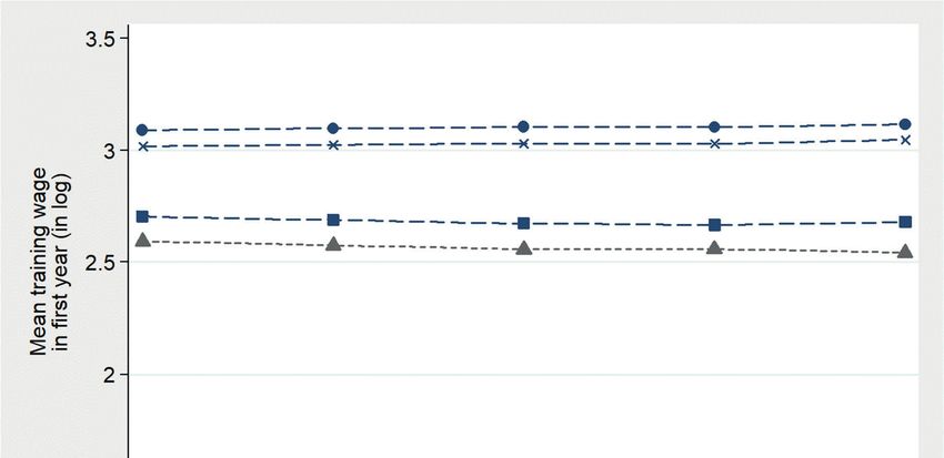
Bibliografische Informationen der Deutschen Nationalbibliothek The Deutsche Nationalbibliothek lists this publication in the Deutsche Nationalbibliografie; detailed bibliographic data are available on the Internet at http://dnb.dnb.de RWI is funded by the Federal Government and the federal state of North Rhine-Westphalia. http://dx.doi.org/10.4419/86788994 ISSN 1864-4872 (online) ISBN 978-3-86788-994-0

Matthias Dorner and Katja Görlitz1

Training, Wages and a Missing School
Graduation Cohort

Abstract
This study analyzes the effects of a missing high school graduation cohort on firms’ training provision and
trainees’ wages. An exogenous school reform varying at the state and year level caused the missing cohort
to occur. Using administrative social security data on all trainees and training firms, we show that firms
provide less training by reducing their overall number of hired apprentices. We also show that the pool of
firms that offer training in the year of the missing cohort shifts towards a higher share of low wage firms.
After keeping firm characteristics constant, the findings indicate that the missing cohort increases training
wages measured at the start of training. Further analyses shed light on the opposite case of dual cohorts,
which we find to increase training provision and to decrease training wages. The evidence also shows
that high and low wage firms differ in how they adjust training provision in response to a dual cohort.

JEL-Code: J21, J24, J31

Keywords: Training wages; training provision; missing high school graduation cohort; high and low wage
firms; dual high school graduation cohort

July 2020

1 Matthias Dorner, IAB Nürnberg; Katja Görlitz, HdBA, IZA, RWI. – Financial support from the German Research
Foundation (DFG) is gratefully acknowledged. The authors thank Ronald Bachmann, Uschi Backes-Gellner, Thomas K. Bauer,
Stefan Bender, Francine Blau, Udo Brixy, Bernd Fitzenberger, Elke Jahn, Sandra McNally, Joachim Moeller, Jens Mohrenweiser,
Uta Schoenberg, Marcus Tamm, Sevrin Waights and Till von Wachter for helpful comments and suggestions. We also
acknowledge comments from participants at conferences and research seminars (Royal Economic Society 2012, Verein für
Socialpolitik 2012, IAB 2012, EALE 2013, First RWI Research Network Conference 2014, IWAEE 2015, FU Berlin 2016, CVER
London 2017, Max-Planck-Institute for Innovation and Competition 2017, University of Regensburg 2018, Committee for the
Economics of Education 2019). We also want to express deep gratitude to Udo Brixy for his particular support of our project.
Matthias Dorner was a research associate at the Institute for Employment Research (IAB) until 2019. All remaining erros are
our own. - All correspondence to: Katja Görlitz, Hochschule der Bundesagentur für Arbeit (HdBA), Seckenheimer Landstr. 16,
68163 Mannheim, Germany, e-mail: katja.goerlitz@hdba.de
1. Introduction

Firms provide apprenticeship training in many countries including Australia, Austria, Canada,
Denmark, Germany, Switzerland and the UK. Apprenticeship training is a successful vocational
pathway for young school leavers to enter the labor market and to keep youth unemployment
low (Lerman 2019). In the US, policy makers formulated the aim of expanding apprenticeship
training starting with the Obama administration.1 Analyzing the mechanisms and functioning
of training markets is essential to understand why firms provide training and what determines
wages of trainees. Gary Beckers’ human capital theory distinguishes between general and firm-
specific training as a key factor to explain why firms provide training (Becker 1962). While
Becker modelled the training decision under perfect competition, another stream of the
literature shows that market imperfections like information asymmetries can equip firms with
monopsony power that allows them to recoup their training investments through their ability to
compress wages (Katz and Ziderman 1990, Chang and Wang 1996, Acemoglu and Pischke
1998, 1999).

This study contributes to the training literature by analyzing the novel research question of
whether the supply of trainees – a factor that the previous literature has largely neglected – is a
determinant of firms’ willingness to provide training and whether it has the potential to affect
trainees’ wages. We investigate the effects of a decrease in the supply of trainees, meaning the
number of school graduates available for an apprenticeship training, that was caused by an
exogenous schooling reform. The reform extended the years required to graduate from high
school from twelve to thirteen years in two German states in the same year. This induced a
missing high school graduation cohort, because the number of high school graduates dropped
virtually to zero in the year after the last “12 years”-cohort had graduated and prior to the first
“13 years”-cohort. The missing cohort decreased the number of potential trainees with high
school degree who could apply for an apprenticeship in the two affected states. Germany is well
suited for our analysis, because firms recruit apprentices on an annual basis mainly from the
pool of current school graduates and two thirds of the German workforce have completed an
apprenticeship program.2 Apprenticeship training combines formal learning in state-funded
vocational schools (for one to two days per week) with working at the training firm (for three
to four days). Firms post vacancies for trainees offering a temporary apprenticeship contract
that includes paying a training wage. If trainees sign an apprenticeship contract, firms employ
them for two to three years at the training firm. While one out of six trainees hold a high school
degree, the majority of trainees have acquired fewer years of schooling. Thus, the missing
cohort induced an exogenous decrease in the supply of high school graduates available for an
apprenticeship.

1
    For an overview of the objectives and initiatives under the former president Obama see
https://obamawhitehouse.archives.gov/the-press-office/2016/04/21/fact-sheet-investing-90-million-through-
apprenticeshipusa-expand-proven (accessed: 2020-06-16). Another example is President Trump‘s executive
order that is issued on June 15, 2017 and available at https://www.whitehouse.gov/presidential-actions/3245/
(accessed: 2020-06-16).
2
  Focusing on the German apprenticeship system also follows Acemoglu and Pischke (1998, 1999) who investigate
it to learn about training processes.

                                                     2
First, we analyze how firms’ training provision developed in the year of the missing cohort,
which we approximate by the number of newly hired trainees. Second, we investigate the effects
of the missing cohort on training wages.3 To identify these effects, we exploit exogenous
variation in the occurrence of the missing cohort by state and year within a difference-in-
difference model. The analysis uses data from administrative social security records available
at the Institute for Employment Research (IAB) that provide accurate information on the
universe of trainees and their training firms.
Analyzing employment and wage responses to a missing cohort also contributes to the literature
explaining how labor markets respond to shifts in labor supply, which is essential to understand
the fundamental question of how labor markets re-equilibrate.4 Most of the previous literature
is concerned with an immigration-induced positive labor supply shock (see e.g. Card 1990,
2001, Pischke and Velling 1997, Borjas 2003, 2006, Manacorda, Manning, and Wadsworth
2012, Ottaviano and Peri 2012, Glitz 2012, Dustmann et al. 2017).5 Other studies address this
topic investigating demographic shocks such as the size of the birth cohorts (Welch 1979,
Berger 1985 and Korenman and Neumark 2000). The study most related to ours is Morin (2015)
who uses micro data to investigate the wage effects of excess supply caused by a schooling
reform that induced two high school cohorts to graduate in the same year. He shows that this
dual cohort decreased weakly earnings significantly. In contrast to Morin (2015) who analyzes
the Canadian labor market, German school graduates usually enter the labor market as trainees
and rarely as unskilled workers. Our study answers the question whether the training market
operates as predicted by the classical labor market model.
The previous theoretical literature describes training as an investment decision of firms who
invest in the productivity of their future workforce and does not predict that supply should affect
training provision (see Becker 1962, Acemoglu and Pischke 1998, 1999). However, trainees
already work in a productive manner during their apprenticeship. Based on German data,
Mohrenweiser and Zwick (2009) show that employing apprentices can increase profits in some
firms, because trainees perform tasks that otherwise unskilled workers would have to conduct.
Thus, firms do not only invest in their workers’ human capital by providing training, but also
demand productive tasks from trainees. Lerman (2019) reviews the international literature on
the training costs of firms. He finds that firms in many countries already recoup much or all of
the costs arising from apprenticeship training through the productive work of their trainees. For
Germany, where many firms report to bear net costs of training, Mohrenweiser and Zwick
(2009) provide evidence that some firms manage to recoup their training costs before the end
3
Wage rigidities could prevent wage adjustments to happen, because wages are subject to collective wage
agreements in Germany. However, firms only have to follow these agreements, if they are part of the employers’
association that negotiates with unions over wages. In 2010, this was the case for 30 percent of the firms only
(Federal Statistical Office 2010). Furthermore, firms can always pay wages exceeding the collective wage
agreements, which is encouraged by the unions. Schnabel and Jung (2011) show that wage cushion is quite
common across German firms. Mohrenweiser et al. (2015) show that training wages can differ within firms for
trainees in the same occupation and year.
4
Another strand of the literature analyzes shifts in labor demand e.g. caused by recessions. See von Wachter and
Bender (2006) for an application exploring the German apprenticeship training system.
5
For an overview, see Dustmann et al. (2016).
3of the training period. Given that there is heterogeneity in the reasons why firms train, where
some firms invest and others produce, our study is complementary to the previous literature.
Besides analyzing the consequence of the missing cohort, we also shed light on the reverse
effect of excess supply in the training market. Shortly after the missing cohort has occurred, the
German federal states decided to abolish the 13th grade. This reform increased the number of
high school graduates to about twice the number of a regular cohort. We are aware of one study
that analyzes the corresponding wage and employment effects in the training market. Based on
aggregate data varying at the state and year level, Mühlemann et al. (2018) find that the dual
cohorts have increased the number of trainees, while they find no evidence of wage adjustments.
We will show that using micro data on trainees and their training firms and applying firm fixed
effects is essential to uncover the mechanisms of adjustments in training wages.
This is because our results indicate that both the missing cohort as well as the dual cohort
induced the average characteristics of training firms to differ from usual years. In particular, we
show that high and low wage firms respond differently. This finding makes an additional
contribution to the literature that is concerned with high and low wage firms and their role in
the development of labor markets (Abowd et al. 1999, Card et al. 2013, Card et al. 2018 and
Song et al. 2019). This literature documents that wage differentials for similar workers across
these two groups of firms exist (Abowd et al. 1999, Card et al. 2013, Card et al. 2018 and Song
et al. 2019). Song et al. (2019) show that much of the rise in earnings inequality derives from
increased wage differentials between firms and not within firms. Little is known about how
high and low wage firms differ in their hiring policies and whether they adjust wages differently
to exogenous shifts in labor supply. In addition, this particular line of heterogeneity across firms
is a novel topic in the context of the training market.
We find that the missing cohort reduced the number of newly hired trainees by at least ten
percent and increased training wages by at least one percent. The latter finding challenges
beliefs of rigid wages in Germany, at least upon first hiring as a trainee. We provide evidence
that composition effects – that occur because trainees hired in the year of the missing cohort
have acquired fewer years of schooling on average – do not influence our wage estimates. The
effects are also robust to alternative calculations of the standard errors and to using a
comprehensive set of model specifications considering time trends, regional covariates and
alternative control states. Our main model and additional empirical analyses show that low
wage firms continued employing trainees in the year of the missing cohort, while high wage
firms stopped doing so. This could be because high wage firms abstain from hiring trainees, if
their applicants do not satisfy the usual hiring criteria such as having a high school degree. In
contrast, the dual cohorts decreased training wages and increased training provision. Our results
further suggest that the dual cohort changed the sample of training firms towards a larger share
of low wage firms. One explanation for this finding is that low wage firms took the unique
opportunity to increase their share of trainees with high school degree, while high wage firms
are always able to attract the desired amount and quality of trainees (unless there is a missing
4cohort). Overall, our findings suggest that shifts in labor supply cause employment and wages
to adjust in accordance with the prediction of the classical labor market model.
The remainder of this study is divided into five sections. The following section briefly outlines
the training system in Germany, describes the school reform that caused the missing high school
graduation cohort to occur and introduces the data. The third section investigates the effects of
the missing cohort on firms’ training provision. Section four presents the wage results and
discusses the role of firm effects. The fifth section presents the analyses and results of the dual
cohort. The final section summarizes the results and draws conclusions.
2. Institutional background and data
2.1 The schooling and apprenticeship training system
The German schooling system is characterized by early tracking that separates students after
primary school based on students’ ability and school performance into three tracks of secondary
education (high school, intermediate track and basic track). The track for the high ability
students leads to a high school degree after 12 years of schooling in some states or after 13
years in others. This difference in the years of high schooling is due to the constitutional
autonomy right of the 16 German federal states to set their own education policy. After school
completion, the majority of high school graduates choose to enroll at university or to apply for
an apprenticeship training. The intermediate track confers a 10th grade certificate and prepares
graduates for an apprenticeship in white-collar occupations. Students from the basic track
graduate after nine years of mostly vocationally oriented secondary schooling, which prepares
them for an apprenticeship in blue-collar occupations. Entering the labor market directly as
unskilled worker is a rare event in Germany for all school leavers. One important reason is that
German law requires all adolescents to participate in the schooling or vocational training system
until the age of 18.
The apprenticeship system combines working in a firm (3-4 days per week) with publicly-
financed vocational schooling (1-2 days).6 Because it is governed at the federal level, there is
no institutional heterogeneity across the 16 states. The curriculum, time schedules, exam
requirements and the duration of training, which usually takes between two and three years, are
constituted by law for each of the more than 400 officially recognized five-digit occupations
(corresponding to 70 three-digit occupations used in this study). School graduates apply for an
apprenticeship at the training firms that decide whom of the applicants to hire on a temporary
training contract for the full duration of the apprenticeship. Training firms remunerate
apprentices with a training wage. As was already mentioned are wages subject to collective
6
Soskice (1994), Harhoff and Kane (1997) and Wolter and Ryan (2011) provide detailed outlines and an
international comparison of the German apprenticeship system.
5wage agreements, which firms have to follow, if they are part of the employers’ association
which was just the case for 30 percent of the firms in 2010 (Federal Statistical Office 2010).
Training wages vary significantly by occupation. For example, occupations that have a higher
share of high school graduates also pay higher wages and provide better employment prospects
measured e.g. in terms of lower unemployment rates and higher wages upon completion of the
apprenticeship. At the end of the training period, firms are free to decide how many of their
trainees they will retain by offering them a long-term employment contract. The average
retention rate is approximately 60 percent (Franz and Zimmermann 2002, Euwals and
Winkelmann 2004, von Wachter and Bender 2006, Göggel and Zwick 2012).
2.2. The missing high school graduation cohort
In 2001, there were no high school graduates available for the apprenticeship market in two
East German states, Mecklenburg-Western Pomerania and Saxony-Anhalt. A major reform of
the high school system caused the missing cohort to occur. In West Germany, attaining a high
school degree uniformly took 13 years of schooling at this time, while these regulations varied
in the five East German states. In the former German Democratic Republic (GDR), high school
required only 12 years of schooling. Two East German states maintained the former
requirements and another state switched to the West German standard shortly after German
reunification in 1990. Mecklenburg-Western Pomerania and Saxony-Anhalt, extended the years
until graduation from 12 to 13 years in the early 2000s. Both states experienced a missing high
school cohort in 2001, because the last cohort graduating after 12 years left high school in 2000
and the first cohort graduating after 13 years left high school in 2002. Figure 1 documents that
the reform caused the number of high school graduates to drop virtually to zero in 2001 in both
states.
6Figure 1: High school graduates by states over time
Source: Kultusministerkonferenz (2007).
Graduates from all school tracks are free to apply for an apprenticeship training in every
occupation, but the occupation-specific composition of trainees by school degree varies
tremendously. To illustrate the extent of this variation, we analyze data from the official
statistics on training contracts.7 Figure A-1 in the Appendix documents that the share of high
school graduates among trainees differ greatly by occupation (Federal Statistical Office 1997,
2000). While many occupations exhibit only a low share of high school graduates of less than
10 percent (most of them being blue-collar jobs), few occupations in the service sector even
have a share of more than 50 percent. This distribution is similar in 1997 and 2000 and, more
generally considered as stable over time. Overall, about 16 percent of apprentices have
previously obtained a high school degree in the period 1997 to 2000 (Federal Statistical Office
1997, 2000).
7
Employers are obliged by law to report each training contract on December 31 to the chambers of industry and
commerce. Because the data is not available at the micro level between 1997 and 2000, we use statistics on the
aggregated number of new training contracts available by year, state and occupation cells that is provided by the
Federal Statistical Office.
7Figure 2 shows that the number of trainees with high school degree declined sharply when the
two states experienced the missing high school cohort in 2001.8 It can also be seen that this
number did not recover to its pre-reform level. This is likely because graduating after 12 years
of high school compared to 13 years affects educational decisions of students. Marcus and
Zambre (2018) find that graduating after 12 years lowered the probability to enroll at university
compared to graduating after 13 years. This effect occurs even though lengthening the years
required for high school had no impact on the overall number of high school graduates
(Huebener and Marcus 2017). For our main analysis of the missing cohort, we restrict our
analysis to the period 1997 to 2001, which is a period in which high schooling required
continuously 12 years. Our empirical model accounts for differences in the high schooling
system across states.
The evidence from Figure 2, indicating that firms hired a lower number of trainees having
graduated from high school, does not necessarily imply that firms provide less training in
general. For instance, firms could anticipate the missing cohort and hire a larger number of
trainees in the year prior to the missing cohort, attract high school graduates from unaffected
states or substitute high school graduates with school leavers not having acquired a high school
degree. Even though it is out of the scope of this study to analyze these adjustment strategies9,
we can show that the missing cohort actually decreased the number of trainees hired. Therefore,
the empirical strategy will provide estimates of the causal effect of the missing cohort on
training provision. This analysis relies on the data introduced in the next section. Analyzing
additionally training provision based on data from the Federal Statistical Office (used in Figure
2) serves the purpose of robustness only. We choose to do so because our main data set allows
us to analyze both training provision and wages, while the data from the Federal Statistical
Office is restricted to the analysis of training provision only because of the lack of individual
wages and firm level information.
8
Figure A-2 in the Appendix documents that the results are similar when showing the corresponding trends
separately for each of the two treated states.
9
When presenting the robustness analyses, we show that there is no evidence of anticipation effects and we further
investigate the role of interstate mobility.
8Figure 2: The development of high school graduates among trainees by states
12
11
high school degree (in log)
Number of trainees with
10
9
8
7
1997 1998 1999 2000 2001 2002 2003 2004 2005
Year
States with a missing high school cohort
Rest of Germany
Source: Federal Statistical Office 1997, 2000
2.3 Data
The analysis exploits administrative micro data recording the universe of employees in
Germany contributing to the social security system, including all trainees. For the purpose of
labor market research, the Institute for Employment Research (IAB) store, process and
anonymize the social security data. The data allows us to identify trainees based on the
mandatory social security employment records that employers have to report to the social
security authorities. From 1999 onwards, trainees can be uniquely distinguished from regular
employees because of a major reform of the reporting system. Prior to that, there was no legally
binding reporting scheme for trainees. Distinguishing trainees perfectly from interns, student
workers or participants in further training is reliable since 1999 only. We address this issue and
harmonize the data over the period 1997 to 2001 by implementing a set of heuristics that were
originally proposed by von Wachter and Bender (2006).10 The analysis of the missing cohort
10
In particular, we exclude individuals who start their training at the age of 30 or older and whose training duration
is shorter than 450 days. We further discard individuals for whom the social security data records regular
employment prior to the first training observation.
9exploits employment records at the reference date June 30 of the years 1997 to 2001. We assign
all trainees being hired between July 1 and next years’ June 30 to the same training cohort.11
The social security data include a comprehensive set of variables covering individuals’
characteristics (e.g. gender, age, schooling degree and nationality), a 3-digit classification of
occupations and, most importantly, precise wage information. Training firms report gross daily
wages with high precision to the social security authorities.12 We deflate wages to 2010 prices
using the consumer price index of the Federal Statistical Office. Even though wages are only
recorded up to a social security contribution limit and are top coded otherwise, this is not an
issue for our study as these limits significantly exceed the wage levels of trainees. In fact, 99.998
percent of the trainees in our data appear to have non-censored wages. The individual records
are complemented with firm characteristics based on unique firm identifiers. Firm
characteristics originate from the IAB Establishment History Panel (BHP) and they were
generated by aggregating the records of the firms’ full workforce (Spengler 2008, Schmucker
et al. 2018).
The firm characteristics cover firm size as measured by the number of employees (including
trainees), the NACE industry classification, the median wage of full-time workers and the skill
composition of the workforce. For the latter, we distinguish the three skill levels: high skilled
employees who have graduated from college or university, medium skilled employees who
have completed an apprenticeship and low skilled employees who have not attained any of these
degrees. Furthermore, the data contain precise geographical identifiers for the location of the
training firms at the level of the federal states (NUTS 1). Based on this information, we can
assign trainees at the start of their training unambiguously to one of the 16 German states. The
data also contains more than 400 counties (NUTS 3) nested within states which is exploited for
running sensitivity checks. The data lacks additional information on the state where trainees
have graduated from school, which prevents us from additionally analyzing school-to-training
mobility across states.
Table A-1 in the Appendix presents summary statistics of the characteristics of trainees and
training firms. While the share of high school graduates among apprentices is 16 percent using
the administrative data from the Federal Statistical Office, Table A-1 shows that it is 13.3
percent in the social security data only. This confirms the previous literature suggesting that
firms’ reports of employees’ education are not as reliable as the other information from the
social security data. Employers tend to report more often the educational degree required by the
average workers in the respective position (Fitzenberger et al., 2006). Since most trainees have
not graduated from high school, the social security data underestimates the actual share of high
school graduates slightly.
11
More than 90 percent of all trainees start their apprenticeship in the second half of the year, of which 80 percent
in the months August and September. This is the period where all school graduates have already finished schooling
in Germany.
12
Although the data contains establishments rather than firms, we refer to them as firms for ease of presentation.
103. The effects of the missing cohort on training provision
3.1 Empirical strategy
We approximate training provision by the number of newly hired trainees in each training
cohort. To analyze whether the missing cohort affects training provision, we aggregate the
micro data of the social security records at the state, year and three-digit occupation level. Each
cell represents the number of newly hired trainees by state, year and occupation. Based on this
data, the following OLS difference-in-difference model is estimated:
Log ሺݏ݁݁݊݅ܽݎݐሻ௦௧ ൌ ߜ ݉݅ݐݎ݄ܿ_݃݊݅ݏݏ௦௧ ߠ௦ ߮௧ ߨ ߝ௦௧ (1)
where log ሺݏ݁݁݊݅ܽݎݐሻ indicates the log of the number of trainees of state s at year t (t=1997-
2001) in occupation o.13 The binary indicator variable ݉݅ ݐݎ݄ܿ_݃݊݅ݏݏtakes the value of one
in the two states that experience a missing cohort in the year 2001 (i.e. in Mecklenburg-Western
Pomerania and Saxony-Anhalt), and zero otherwise. The remaining 14 German states constitute
the control group taking economic or policy changes into account that are common to all
German states. The regression includes state fixed effects (ߠ) to account for statewide
difference in the high school system and in training provision. Year fixed effects (߮) absorb
changes in economic conditions and occupation fixed effects (ߨ) control for the occupation-
specific variation of the share of high school graduates among trainees (see again Figure A-1).
The indicator ߝ represents the idiosyncratic error term. To account for the significant
differences in the size of the labor market by states, we weight the regressions by the state-
specific number of trainees. The coefficient ߜ is the parameter of interest that identifies the
lower bound of the missing cohort on training provision. One reason why we can only identify
a lower bound is that our data does not observe high school graduates from other states to apply
at the states with the missing cohort.14
Starting with Bertrand et al. (2004), there is a large debate on how to calculate standard errors
in difference-in-difference applications when using micro data. When presenting wage
estimates, we discuss this literature in detail. However, it is not of importance for our analysis
of training provision because the analysis relies on aggregated and not on micro data. Inference
is based on the model suggested by Donald and Lang (2007). As was already noted will we
aggregate our main data from the social security system at the state, year and occupation level
when estimating Equation (1). Additionally, we will estimate Equation (1) based on the data
13
Table A-2 in the Appendix presents summary statistics of the log of the number of trainees by state and year in
the first two columns.
14
The difference-in-difference estimator can be calculated as (ignoring occupation, state and year fixed effects to
keep it as simple as possible): ߜ ൌ ሾܧሺlogሺݏ݁݁݊݅ܽݎݐሻ௦௧ | ݉݅ ݐݎ݄ܿ_݃݊݅ݏݏൌ 1, ݎܽ݁ݕଶଵ ൌ 1ሻ െ
ܧሺlogሺݏ݁݁݊݅ܽݎݐሻ௦௧ | ݉݅ ݐݎ݄ܿ_݃݊݅ݏݏൌ 1, ݎܽ݁ݕଶଵ ൌ 0ሿ െ ሾܧሺ ܧlogሺݏ݁݁݊݅ܽݎݐሻ௦௧ | ݉݅ ݐݎ݄ܿ_݃݊݅ݏݏൌ
0, ݎܽ݁ݕଶଵ ൌ 1ሻ െ ܧሺ ܧlogሺݏ݁݁݊݅ܽݎݐሻ௦௧ | ݉݅ ݐݎ݄ܿ_݃݊݅ݏݏൌ 0, ݎܽ݁ݕଶଵ ൌ 0ሻሿ. We expect the sign of ߚመ to be
negative. In this setting, mobility induces the first term to increase (as more school graduates apply in the treated
states), while the second term decreases (as the school graduates leave from the control states). The effect of the
missing cohort is attenuated towards zero.
11provided by the Federal Statistical Office which is only available in aggregated form and which
was already used in Figure 2. While both sources contain administrative information on the
total population of trainees, they differ in the administrative process of reporting including the
institutions where firms have to report to, the reference period and the exact unit of observation
(number of hired trainees in the social security data versus training contracts).
3.2 Results on training provision
Using data from the social security records, Table 1 shows in the first column that firms train
approximately ten percent fewer trainees in response to the missing cohort. The second column
contains the sensitivity analysis estimating Equation (1) based on the data from the Federal
Statistical Office. These results also show that firms have signed ten percent fewer training
contracts.15 This is an astonishing result given the great extent of differences in the reporting
scheme of both data sets.
Table 1: The effect of the missing cohort on training provision
Log of the number
of trainees
(1) (2)
The effect of the missing cohort -0.102 *** -0.104 ***
(0.020) (0.025)
Adj. R2 0.939 0.945
Obervations 6,443 5,305
Notes: The dependent variable is the log of the number of trainees. Column (1) presents
estimates of Equation (1) using the data from the social security system aggregated at the state,
year and occupation level. Column (2) present estimates of Equation (1) using the aggregated
data from the Federal Statistical Office. The standard errors are shown in parentheses. Statistical
significance: p4. The effects of the missing cohort on training wages
4.1 Empirical strategy
The analysis of training wages also employs a differences-in-differences design that uses
exogenous variation in the missing cohort by state and year. We estimate the following linear
regression model (that we henceforth refer to our baseline model):
Log(wܽ݃݁ሻ௦௧ ൌ ߚ ݉݅ݐݎ݄ܿ_݃݊݅ݏݏ௦௧ ߩ௦ ߛ௧ ߥ௦௧ (2)
where log ሺ݁݃ܽݓሻ indicates the log training wage of individual i starting training in state s at
year t (t=1997-2001).16 Again, the binary indicator variable ݉݅ ݐݎ݄ܿ_݃݊݅ݏݏis 1 in the two
states with the missing cohort in the year 2001, and zero otherwise. As before, the analysis uses
the rest of Germany to control for statewide economic or policy shocks. The regression includes
state fixed effects (ߜ) that captures unobserved time-invariant state characteristics that could be
correlated with training wages like differences in the economic environment or policy
differences across states.17 The year fixed effects (ߩ) absorb contemporaneous events common
to all states like the business cycle. The indicator ߥ represents the idiosyncratic error term. The
coefficient ߚ pools three potential mechanisms together that might have opposite effects on
wages. This is because the missing cohort could affect wages through different channels.
First, it reduces the labor supply of trainees by which it should raise wages according to the
classical labor market model (supply effect). This model also predicts that the missing cohort
reduces the number of trainees, which we already documented in the previous section. Second,
the composition of trainees has changed, because of a lower average schooling level. This
composition effect could reduce average wages of the 2001 cohort. Third, the missing cohort
could also mirror firm effects. Firm effects would matter, if the missing cohort reduces the
number of trainees mainly in firms that pay higher or lower training wages. We consider this
as likely because the missing cohort did not only decrease the size of the pool of training
applicants, but it also decreased the average schooling quality of the applicants. If high wage
firms offer training more often to high school graduates, the missing cohort would affect high
wage firms more severely. If mostly these firms decided to offer less training in the year of the
missing cohort, because they were unable to fill their open slots with the “usual” candidates,
firm effects induce average wages to decrease in the year of the missing cohort.18 In the opposite
case of negative assortative matching of labor market entrants into training firms, low wage
firms would have stopped hiring trainees more often.
16
Table A-2 in the Appendix presents summary statistics of log wages at start of training by states and year.
17
Introducing state fixed effects seems sufficient to consider state-specific wage differentials because Figure A-3
in the Appendix illustrates that these differentials mainly represent levels and not time trends. Further robustness
tests controlling for time trend support this conclusion.
18
This would assume positive sorting of workers into firms. The empirical literature has not yet reached consensus
on whether positive or negative sorting exists (Abowd et al. 1999, Andrews et al. 2008, Eeckhout and Kircher
2011, Andrews et al. 2012, Card et al. 2013 and Ehrl 2019). The evidence on Germany is also mixed. While some
previous studies conclude negative sorting to be apparent (Andrews et al. 2007, 2012), more recent studies by Card
et al. (2013) and Ehrl (2019) provide evidence of positive assortative matching.
13To disentangle the supply effect from the composition effect, we will proceed stepwise. To find
out how much the composition effect contributes to the estimated wage results, we amend
Equation (2) to control for trainees’ characteristics, in particular, for the schooling degree, age,
gender and nationality. Occupation fixed effects will be included in the regressions at the 3-
digit level to account for the considerable occupational-specific heterogeneity regarding the
share of high school graduates. These regressions only present suggestive evidence because
changes in the individual characteristics directly stem from the reform itself. Therefore, we
present findings from the literature and run an additional empirical analysis, supporting our
conclusion that composition effects do not matter in our application.
To find out how much observable firm characteristics matter, we proceed in the same manner
as with our analysis of composition effects. Equation (2) additionally controls for time-varying
characteristics such as firm size, the median of wages of full-time workers, the skill composition
of the workforce and firms’ industry affiliation (at the level of 17 NACE sections). Observing
all training firms in Germany in our data allows us additionally to apply firm fixed effects to
absorb all time-invariant firm characteristics that might influence training wages. Importantly,
we will show that applying firm fixed effects absorb both time-invariant and time-varying firm
effects.
The following model, henceforth referred to our main model, considers firm fixed effects:
log ሺ݁݃ܽݓሻ ൌ ߟ ݉݅ݐݎ݄ܿ_݃݊݅ݏݏ௦௧ ߤ௧ ߙ ߱௦௧ . (3)
The variables log ሺ݁݃ܽݓሻ and ݉݅ ݐݎ݄ܿ_݃݊݅ݏݏwas already described when presenting the
baseline model. ߤ௧ represents the vector of year fixed effects and ߙ represents the firm fixed
effects where j indicates the training firm.19 ߱ represents the idiosyncratic error term. The
estimate of ߟ displays the supply effect of the missing cohort on wages (given that we will show
that composition effects are not an empirical issue and that firm fixed effects are sufficient to
control for differences in firm characteristics). Again, ߟ represents a lower bound because of
the mobility-induced attenuation bias. Section 4.3 provides further empirical evidence on the
extent of this bias by controlling in parts for mobility.
Comparison of the baseline estimates from Equation (2) and the main estimates from Equation
(3) sheds light on the question whether the missing cohort affects high and low wage firms
differently. If Equation (3) were the true model, the baseline estimate ߚመ would be calculated as
(leaving out other controls for ease of exposition):
ܿݒሺ݉݅ݐݎ݄ܿ_݃݊݅ݏݏ, ߙ݆ ሻ
ߚ ݈݉݅መ ൌ ߟ
ݎܽݒሺ݉݅ݐݎ݄ܿ_݃݊݅ݏݏሻ . (4)
19
State fixed effects cannot be considered in addition because firms are almost entirely nested within states, leaving
insufficient variation for identification.
14If ߚመ and ߟƸ were the same (for ܿݒ൫݉݅݃݊݅ݏݏ௧ , ߙ ൯ ൌ 0), the missing cohort would reduce
the number of trainees homogenously in all firms, meaning the missing cohort would be
unrelated to firm characteristics. If ߚመ ൏ ߟƸ , the latter term of Equation (4) would become
negative. This would happen, if the share of low (high) wage firms increases (decreases) among
training firms in response to the missing cohort. If ߚመ ߟƸ , the opposite would be the case. To
reinforce our conclusion drawn from comparing ߚመ and ߟƸ , further robustness analyses provide
more direct evidence on the effects of the missing cohort on the characteristics of training firms
and on the provision of training by high and low wage firms.
Clustering of standard errors and inference
In their seminal paper, Bertrand et al. (2004) emphasized the importance of the choice of
method of estimating standard errors in differences-in-differences applications. Standard errors
are likely downward biased when the errors are serially correlated over time or within units
(Moulton 1990). In general, Abadie et al. (2017) highlight that the choice of the clustering unit
for the standard errors should be aligned with the experimental design of each study. Following
this literature, we cluster standard errors at the state level in our main model analyzing training
wages. Another issue hotly debated is how to proceed in settings with only few clusters as in
our case where the highest level of aggregation allows clustering at only 16 German states (see
Donald and Lang 2007, Cameron et al. 2008, Conley and Taber 2011). Donald and Lang (2007)
as well as Cameron et al. (2008) suggest applying alternative critical t-values for inference that
can at least reduce the bias in samples with few clusters, which we implement additionally.20
Furthermore, adjusting standard errors by combinations of the unit structure and time
dimensions, i.e. units by years or pre-/post-period, represents another multi-way cluster-robust
approach practiced in the literature (Donald and Lang 2007). For reason of sensitivity, we
present a variety of alternative calculations of the cluster-robust standard errors.
As an alternative to the cluster-robust inference, Cameron et al. (2008) recommend applying
the wild cluster bootstrap to eliminate bias. This cluster-robust variance estimator allows for
unrestricted intra-group correlation in differences-in-differences settings and is
heteroscedasticity robust. We will implement this approach as a test of robustness for our main
model. However, in settings with few treated states as in our main analysis where we only have
two treated out of 16 states, MacKinnon and Webb (2017) document that the desirable
properties of the approach do not hold and instead lead to unreliable statistical inference.
Precisely, the wild cluster bootstrap will produce inference that overrejects the null hypothesis.
To find out whether overrejection is apparent in empirical applications, Roodman et al. (2019)
suggest implementing a version of the wild cluster bootstrap with restricted and unrestricted
heteroscedasticity and, then, compare the conformity of the two estimates. As a rule of thumb,
the wild cluster bootstrapped standard errors would be problematic, if the inference from the
20
They suggest t(G-1) or t(G-2), with G denoting the number of clusters in the data.
15restricted and the unrestricted model differ from another. In these cases, MacKinnon and Webb
(2018) suggest the subcluster wild bootstrap to improve reliability of inference. This approach
draws on wild bootstraps that are performed at levels of subunits in nested data. As we observe
counties in which training firms are located in our data set that are unambiguously nested in the
16 federal states, we perform the suggested approach at the level of the 401 counties.
4.2 Results on training wages
Table 2 shows the baseline results without applying firm fixed effects using the log training
wage at start of training as dependent variable. The estimate is significantly negative,
suggesting the missing cohort to decrease wages by four percent. Including trainee
characteristics does only modestly alter the estimate as can be seen from column (2). This result
is astonishing given that the missing cohort reduced the average schooling level of trainees. We
suggest that the most likely reason for this finding is that training wages are only slightly higher
for high school graduates compared to school leavers without having acquired a high school
degree.21
Column (3) indicates that considering occupation fixed effects only slightly decreases the
estimate of the missing cohort, but leaves its sign and significance unchanged. In contrast,
controlling for log firm size, the median of wages, the skill composition of the firms’ workforce
and industry identifiers alters the estimate noticeably. The estimate decreases by the factor ten
and is no longer statistically distinguishable from zero. This suggests that firm characteristics
need to be held constant when analyzing the effect of the missing cohort on wages of trainees.
21
Pischke and von Wachter (2008) find that increasing schooling by one more year has zero wage returns in
Germany. They explain their result by the German schooling system in which basic vocational skills - that are
essential for successful completion of an apprenticeship - are already learned by grade 8 regardless of school track.
Even though high school graduates attend school longer than their counterparts in the lower tracks, their additional
skills and knowledge do prepare them for subsequent academic education, but might not provide large productivity
advantages in the training period. To shed more light on this suggestion, we regress the log starting wage on a
dummy being 1 for high school graduates and 0 for all other school degrees. These results show that high school
graduates earn only three percent higher wages at the start of training compared to other school graduates.
16Table 2: Baseline results of the effect of the missing cohort on training wages
Log training wage
(1) (2) (3) (4)
The effect of the -0.040 *** -0.037 *** -0.029 ** -0.003
missing cohort (0.013) (0.011) (0.013) (0.007)
Trainee characteristics No Yes Yes Yes
Occupation fixed effects No No Yes Yes
Firm characteristics No No No Yes
2
Adj. R 0.264 0.319 0.538 0.711
Obervations 2,151,726 2,151,726 2,151,726 2,151,726
Notes: OLS results of our baseline specification that incorporate a dummy for the missing
cohort in addition to state and year fixed effects (see Equation (2)). Trainee characteristics cover
gender, age, German nationality and high school degree (y/n). Occupation fixed effects are
introduced at the 3-digit level. Firm characteristics indicate log firm size, median of wages of
full-time employees, the skill composition of the workforce (high, medium and low skilled
worker shares) and 17 NACE industry sections. Standard errors shown in parentheses are
clustered at the state level. Significance levels: *** 1%, ** 5%.
Source: Social security data
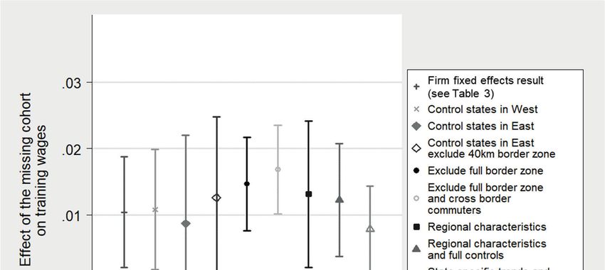
Table 3 illustrates our main results applying firm fixed effects where the first column again
shows the baseline results from column 1 of Table 2 for reason of comparison. Column (2)
documents that the lower bound effect of the missing cohort on wages of trainees is one percent
once taking firm fixed effects into account. This result remains the same after controlling for
trainee characteristics, occupation fixed effects or time-varying firm characteristics (see
Column (3) and (4)). This suggests that the firm fixed effects already cover all factors that
correlate with training wages and the missing cohort. Comparing the results from the baseline
with the fixed effects model shows that ߚመ ൏ ߟƸ , which is evidence that the missing cohort
induced a negative selection of training firms. This could be either because firms with inferior
characteristics and low wages kept hiring trainees, while firms with superior characteristics and
higher wages stopped to provide training. Alternatively, it could also be that both high and low
wage firms decreased training provision, but the former reduced it to a greater extent. The
following two paragraphs answer this question and provide further sensitivity analyses
supporting our conclusion that the missing cohort affects the quality of the average training
firm.
17Table 3: Firm fixed effects results of the effect of the missing cohort on training wages
Log training wage
(1) (2) (3) (4)
The effect of the -0.040 *** 0.010 ** 0.010 *** 0.010 ***
missing cohort (0.013) (0.004) (0.003) (0.003)
Firm fixed effects No Yes Yes Yes
Trainee characteristics No No Yes Yes
Occupation fixed effects No No Yes Yes
Firm characteristics No No No Yes
Adj. R2 0.264 0.907 0.919 0.919
Obervations 2,151,726 2,151,726 2,151,726 2,151,726
Notes: Column (1) reports again the baseline results from Table 2. Column (2) documents the
firm fixed effects estimates that incorporate a dummy for the missing cohort in addition to year
and firm fixed effects (see Equation (3)). Columns (3) and (4) stepwise include further controls.
Trainee characteristics cover gender, age, German nationality and high school degree (y/n).
Occupation fixed effects are introduced at the 3-digit level. Firm characteristics indicate log
firm size, median of wages of full-time employees, the skill composition of the workforce (high,
medium and low skilled worker shares) and 17 NACE industry sections. Standard errors shown
in parentheses are clustered at the state level. Significance levels: *** 1%, ** 5%.
Source: Social security data
First, we document which firms kept hiring trainees in the year of the missing cohort by
regressing several firm characteristics on a the treatment dummy in addition to state and year
fixed effects. The dependent variables the log firm size, the log median wage and the shares of
high, medium and low skilled workers are investigated with a one-year lag in order to describe
changes in firm characteristics.22 Table 4 documents that training firms that usually employ a
larger share of low skilled workers and a lower share of medium and high skilled workers were
more likely to provide training in the year of the missing cohort.
22
Investigating firm characteristics in 2001 would answer another question that is out of the scope of this study,
meaning e.g. whether firms have hired a larger number of low or medium skilled workers to compensate for the
missing high school graduation cohort.
18Table 4: Characteristics of training firms and the missing cohort
Share of
Log Log medium
low skilled high skilled
firm size median wage skilled
workers workers
workers
(1) (2) (3) (4) (5)
The effect of the -0.017 -0.013 0.025 *** -0.017 *** -0.007 **
missing cohort (0.036) (0.009) (0.003) (0.005) (0.003)
2
Adj. R 0.022 0.158 0.082 0.103 0.022
Obervations 1,188,146 1,188,146 1,188,146 1,188,146 1,188,146
Notes: The dependent variables that are measured with a one-year lag are shown in the first
row. The number of observations differs from Table 3, because the regression is conditional on
the training firm being active in the previous year. All training firms in 1997 had to be deleted
additionally because there is no pre-year information. Low skilled workers have not obtained a
vocational degree, medium skilled workers have successfully completed an apprenticeship and
high skilled workers have graduated from university or college. Standard errors shown in
parentheses are clustered at the state level. Significance levels: *** 1%, ** 5%.
Source: Social security data
Second, we analyze how high and low wage firms hired trainees in the year of the missing
cohort. To do so, we calculate the residuals from a firm level regression of the log training wage
on log firm size, the skill composition of the workforce, industry, year and states dummies for
the pooled period 1997 to 2000 for every firm with at least one training record during this
period. Taking the mean of the residuals for every firm allows us to observe each firms’ position
in the training wage distribution adjusted for firm and workforce characteristics. We define high
and low wage firms based on quartiles (but also on tertiles for reason of robustness). High wage
firms represent the top quartile (tertile) and low wage firms represent the lower quartile (tertile).
To analyze how high and low wage firms provide training, we follow our previous analysis of
training provision and calculate the overall number of trainees hired by state, year and
occupation cells as well as by high and low wage firms.23 Using this data, the log of the number
of trainees is regressed on a binary indicator of the missing cohort, state, year and occupation
fixed effects in separate regressions distinguishing high and low wage firms. As before, the
regressions consider weights to account for differences in the size of the state’s labor market.
Column (1) and (3) of Table 5 illustrates that low wage firms did not modify the number of
hired trainees in response to the missing cohort. In contrast, columns (2) and (4) documents that
high wage firms reduced hiring trainees by about 17 percent (exp((െ0.192)-1)*100) to 20
percent (exp((െ0.232)-1)*100). Taken all the evidence from Table 3 to 5 together, we conclude
23
Because of aggregating the data, the number of observations differ slightly between using quartiles or tertiles.
19that particularly firms with superior characteristics decided not to hire as many trainees as
usually when facing a missing cohort.
Table 5: Training provision by high and low wage firms
Log of the number of trainees
High wage High wage
Low wage firms Low wage firms
firms firms
(quartiles) (tertiles)
(quartiles) (tertiles)
(1) (2) (3) (4)
The effect of the -0.006 -0.192 ** -0.017 -0.232 ***
missing cohort (0.063) (0.074) (0.062) (0.074)
Adj. R2 0.855 0.851 0.878 0.878
Obervations 5,555 5,312 5,766 5,611
Notes: The dependent variable is the log of the number of trainees. See more information on
the empirical proceeding in the text. Standard errors shown in parentheses are clustered at the
state level. Significance levels: *** 1%, ** 5%.
Source: Social security data
4.3 Robustness analyses of the main wage results applying firm fixed effects
Clustering of the standard errors
To assess whether clustering of the standard errors affects the statistical inference of our main
effects, we vary the level and type of clustering. Table 6 summarizes the results. Panel A shows
again the main results in parentheses where inference applies cluster-robust standard errors at
the state level adjusted for a small number of state clusters. This seems important given that the
results from Panel B point out that the standard errors are underestimated without clustering at
the state level. Before presenting the results of the wild cluster bootstrap (shown in brackets),
we compare our main results with the subcluster-robust inference that are indicated in
parentheses. Panel C to E shows results clustering at the county level (401 clusters), at the states
ൈ year level (80 clusters) and at the level of states ൈ pre-/post-indicator (32 clusters),
respectively. These findings confirm the statistically significance of our main results.
Next, we discuss the results when applying the wild cluster bootstrap (WCB). Panel A shows
that the p-values of the restricted and the unrestricted WCB model lead to ambiguous
conclusions about the estimates’ statistical significance. Such an ambiguous finding suggests
20that the WCB approach is not valid in cases with few treated clusters only as apparent in our
analyses (Roodman et al. 2019). In such cases, MacKinnon and Webb (2018) recommend
instead estimating the WCB clustered at a finer level of aggregation. Clustering at the level of
401 counties, which leads to 26 treated units, brings the inference from the restricted and the
unrestricted WCB in accordance (see Panel C) and shows our findings to differ significantly
from zero. Subclustering wild bootstraps at the level of combinations between state and year as
in Panel D and E is not superior to clustering at the county level because the restricted and the
unrestricted model are not in line with each other. One likely reason for this is that these models
also consider only an insufficiently small number of treated units.
These findings suggest that the restricted WCB model clustered at the state level (Panel A)
overrejects the null hypothesis in our setting. To shed further light on this issue, section 5
presents the results from the dual cohorts, i.e. high school cohorts that are twice as large as
usually occurring in as much as 13 states between 2007 and 2016. The analysis finds statistically
significantly results of both the restricted and the unrestricted WCB irrespectively of clustering
at the state, county or any combinations of the state and year level. This supports our conclusion
that the WCB does not work well when analyzing the effects of the missing cohort because of
too few treated units.
21You can also read