PVBM: A Python Vasculature Biomarker Toolbox Based On Retinal Blood Vessel Segmentation
←
→
Page content transcription
If your browser does not render page correctly, please read the page content below
PVBM: A Python Vasculature Biomarker
                                                 Toolbox Based On Retinal Blood Vessel
                                                             Segmentation

                                         Jonathan Fhima1,2 , Jan Van Eijgen3,4 , Ingeborg Stalmans3,4 , Yevgeniy Men1,5 ,
                                                            Moti Freiman1 , and Joachim A. Behar1
arXiv:2208.00392v1 [cs.CV] 31 Jul 2022

                                                       1
                                                         Faculty of Biomedical Engineering, Technion-IIT, Haifa, Israel
                                                   2
                                                        Department of Applied Mathematics Technion–IIT, Haifa, Israel
                                               3
                                                   Research Group Ophthalmology, Department of Neurosciences, KU Leuven,
                                                                                  Belgium
                                                 4
                                                    Department of Ophthalmology, University Hospitals UZ Leuven, Belgium
                                             5
                                                 The Andrew and Erna Viterbi Faculty of Electrical & Computer Engineering,
                                                                         Technion–IIT, Haifa, Israel

                                                 Abstract. Introduction: Blood vessels can be non-invasively visual-
                                                 ized from a digital fundus image (DFI). Several studies have shown an
                                                 association between cardiovascular risk and vascular features obtained
                                                 from DFI. Recent advances in computer vision and image segmentation
                                                 enable automatising DFI blood vessel segmentation. There is a need for a
                                                 resource that can automatically compute digital vasculature biomarkers
                                                 (VBM) from these segmented DFI. Methods: In this paper, we intro-
                                                 duce a Python Vasculature BioMarker toolbox, denoted PVBM. A total
                                                 of 11 VBMs were implemented. In particular, we introduce new algorith-
                                                 mic methods to estimate tortuosity and branching angles. Using PVBM,
                                                 and as a proof of usability, we analyze geometric vascular differences be-
                                                 tween glaucomatous patients and healthy controls. Results: We built a
                                                 fully automated vasculature biomarker toolbox based on DFI segmen-
                                                 tations and provided a proof of usability to characterize the vascular
                                                 changes in glaucoma. For arterioles and venules, all biomarkers were sig-
                                                 nificant and lower in glaucoma patients compared to healthy controls
                                                 except for tortuosity, venular singularity length and venular branching
                                                 angles. Conclusion: We have automated the computation of 11 VBMs
                                                 from retinal blood vessel segmentation. The PVBM toolbox is made open
                                                 source under a GNU GPL 3 license and is available on physiozoo.com
                                                 (following publication).

                                                 Keywords: Digital fundus images, digital vascular biomarkers, glau-
                                                 coma, retinal vasculature

                                         1     Introduction

                                         According to the National Center for Health Statistics, cardiovascular diseases
                                         (CVD), including coronary heart disease and stroke, are the most common cause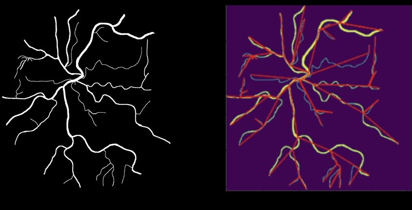
2                                Fhima J. et al.

of death in the USA [35]. Since the beginning of the 20th century, researchers
have shown that retinal microvascular abnormalities can be used as biomark-
ers of CVD [15,16,23]. Retinal vasculature can be non-invasively assessed using
DFIs, which can be easily obtained using a fundus camera. Consequently, retinal
vascular features obtained from DFI may be used to characterize and analyze
vascular health. In order to enable reproducible research, it is necessary to fully
automate the computation of these biomarkers from the segmented vasculature.
We developed a Python Vasculature Biomarker Toolbox (PVBM), based on DFI
segmentations made by expert annotators from the University Hospitals Leuven
in Belgium. PVBM enables a quantitative analysis of the vascular geometry
thereof with broad application in retinal research. In this paper we illustrate the
potential of PVBM by characterizing vascular changes in glaucoma patients.

1.1   Prior works

Connection between retinal vasculature and cardiovascular health: As
early as of beginning of the 20th Century research has been carried out to as-
sess the relationship between the retinal vasculature and cardiovascular health.
Marcus Gunn can be seen as one of the first to describe the relation between
hypertension and retinal characteristics [15,16], and is followed by the work of
H.G Scheie [43] in 1953. In 1974, N.M Keith showed that hypertension and its
mortality risk is reflected in the retinal vasculature [23] and in 1999 Sharrett et
al. [44] added arterio-venous nicking and arteriole narrowing to the list of patho-
logical findings. Examples of retinal microvascular abnormalities in hypertensive
patients can be seen in Fig. 1. Witt et al. [50] concluded that vessel tortuos-
ity significantly distinguished between patients with ischemic heart disease and
healthy controls. Over the years retinal vessel calibres were shown to change in
hypertension [4], obesity [18], chronic kidney disease [33,42], diabetes mellitus
[4], coronary artery disease [17] and glaucoma [22]. Fractal dimensions of the reti-
nal vascular tree are among the newest biomarkers to study cardiovascular risk.
Monofractal dimension was shown to change with age, smoking behaviour [24],
blood pressure [27], diabetic retinopathy [6], chronic kidney disease [45], stroke
[9], and coronary heart disease mortality [25], while Multifractal dimensions were
found to be negatively associated with blood pressure and WHO/ISH cardiovas-
cular risk score [49]. The established association between vascular biomarkers
and CVD prompts the development of algorithmic solutions for automated com-
putation thereof.

Automated biomarker computation based on DFIs: Several attempts
have been made to extract meaningful biomarkers to characterize cardiovascu-
lar health based on DFI vasculature. In 2000, Martinez-Perez et al. [32] intro-
duced a semi-automated algorithms capable of computing vasculature biomark-
ers (VBMs) such as vessel diameter, length, tortuosity, area and branching an-
gles. In 2011, Perez-Rovira et al. [38] created Vessel Assessment and Measure-
ment Platform for Images of the REtina (VAMPIRE), a semi-automatic software
PVBM          3

Fig. 1. Examples of retinal vascular signs in patients with cardiovascular diseases.
Reproduced with permission from Liew et al. [26] . Black arrow: focal arteriolar nar-
rowing, White arrow: arterio-venous nicking, Yellow arrow: haemorrhage, Blue arrow:
micro-aneurysm, Red arrow: cotton wool spot.

that can extract the optic disk and compute vessel width, tortuosity, fractal di-
mension, and branching coefficient. RetinaCAD was developed in 2014 [8]. This
automated system is able to calculate Central Retinal Arteriolar Equivalent
(CRAE), the Central Retinal Venular Equivalent (CRVE), and the Arteriolar-
to-Venular Ratio (AVR). Lastly, many algorithmic approaches have been devel-
oped to estimate the blood vessel tortuosity [19,14,36]. Last year, Provost et al.
[40] used the MONA REVA software which semi-automatically segments retinal
blood vessels and measures tortuosity and fractal dimension in order to analyze
the impact of their changes on children’s behaviour.

1.2   Research gap and objectives
Vasculature biomarkers have been previously proposed and implemented in a
semi or fully automated manner. However, these biomarkers were only analyzed
individually across multiple groups. Hence the need to use a combined, com-
prehensive set of VBM within a machine learning (ML) framework for disease
diagnosis and risk prediction. The large number of images needed to train ML
algorithms require a fully automated computation of these VBM. In this paper
we created a computerized toolbox, denoted PVBM, that enables the compu-
tation of 11 VBMs engineered from segmented arteriolar or venular networks.
A potential application of PVBM is demonstrated by comparison of VBM in
glaucoma patients versus healthy controls.

2     Methods
2.1   Dataset
A database provided by the University Hospitals of Leuven (UZ) in Belgium was
used. This database contains 108,516 DFIs, centered around the optic disc. The
4 Fhima J. et al.
Table 1. Leuven A/V segmented database (UZFG) summary including the median
(Q1-Q3) age, the gender and the diagnosis for the glaucoma (GLA) patient and normal
ophthalmic findings (NOR) patient.
No DFIs Age Gender
NOR 19 58(43-60) 42% M
GLA 50 68(59-75) 42% M
Total 69 61(57-70) 42% M
resolution of 1444×1444 is higher than most public databases, which enables the
visualization of smaller blood vessels. Median age was 66 (Q1 and Q3 respectively
54 and 75 years old) and 52% were women. For a subset of the database, the
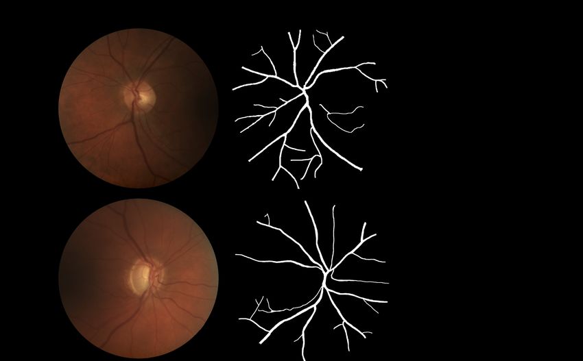
blood vessels were manually segmented by retinal experts using Lirot.ai on Apple
iPad Pro 11”and 13” [12]. This subset is denoted UZFG and consists of 69 DFIs.
The patients included in UZFG were between 19 and 90 years old with a median
age of 61 (Q1 and Q3 were 57 and 70 years old), 58% were female. UZFG has
59% of left and 41% of right eye DFIs. Patients belonging to the UZFG are
separated into the classes: Normal ophthalmic findings (NOR) and Glaucoma
(GLA).
Protocol for DFI vasculature segmentation by experts: Arterioles carry
higher concentration of oxyhemoglobin than venules and therefore exhibit a
brighter inner part compared to their walls. This feature is known as the cen-
tral reflex and is more typical for larger arterioles [34]. The exact intensity of
this reflection is additionally influenced by the composition of the vessel wall
[21], the roughness of the surface, the caliber of the blood column, the indices
of refraction of erythrocytes and plasma, the pupil size, the axial length of the
eye and the tilt of the blood vessel relative to the direction of incident light.
Since the branching of arterioles and venules can be found inside the optic nerve
head, two arterioles or venules can be found adjacently at the optic disc rim
[5]. The image variability in term of color, contrast, and illumination, challenge
an accurate (automatic) arteriole-venule discrimination [3]. Vessel segmentation
was manually performed by a pool of ten ophthalmology students experienced in
microvascular research, using the software Lirot.ai [12] and afterwards corrected
by an UZ retinal expert. Arteriole-venule discrimination was carried out based
on the following visual and geometric features [34]:
– Venules are darker than arterioles.
– The central reflex is more recognizable in arterioles.
– Venules are usually thicker than arterioles.
– Venules and arterioles usually alternate near the optic disc.
– It is unlikely that arterioles cross arterioles or that venules cross venules.
2.2 Digital vasculature biomarkers
A total of 11 VBMs were implemented in PVBM (Table 2). The biomarkers were
computed separately for arterioles and venules.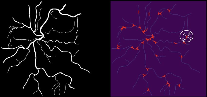
PVBM    5

       Table 2. List of digital vasculature biomarker implemented in PVBM.

                 Number                           Biomarker         Definition                Unit
                    1                            OVLEN[32]        Overall length             Pixel
                    2                            OVPER[32]      Overall perimeter            Pixel
                    3                            OVAREA[32]        Overall area              Pixel2
                    4                              END[32]     Number of endpoints             -
                    5                             INTER[32] Number of intersection points      -
                    6                             TOR[32,28]    Median tortuosity              %
                                                                                          o
                    7                               BA[32]       Branching angles           (degree)
                    8                              D0 [46,7]   Capacity dimension              -
                    9                              D1 [46,7]    Entropy dimension              -
                   10                              D2 [46,7]  Correlation dimension            -
                   11                               SL[29]      Singularity Length             -

Fig. 2. Skeletonization process of a vascular network. (A): Example of a vascular net-
work ya , (B): Corresponding skeleton of ya .

Overall length: The OVLEN biomarker refers to the sum of the length of a
vascular network, whether for arterioles or venules. To compute it, the first step
is to extract the skeleton of the vascular network, which can be seen in fig. 2.
Then the number of pixels that belong to this skeleton are summed, and divided
by the image size (1444x1444), then multiplied by 1000 for scaling purposes. It
is computed using the following formula:

          OVLEN = 1e3*\frac {\Sigma _{p \in S} \sqrt {2}*\mathbb {1}_{|\partial _x p| + |\partial _y p| = 0}(p) + \mathbb {1}_{|\partial _x p| + |\partial _y p| \neq 0}(p)}{1444^2}           (1)

where S is the set of pixel inside the skeletonized image (Fig.2), and x/y represent
the horizontal/vertical direction.

Overall perimeter: The OVPER refers to the sum of perimeter’s length of
a vascular network. It is computed as the length of the border of the overall
segmentation. It required an edge extraction of the segmentation, which could
be easily found by convolving the original segmentation by a Laplacian filter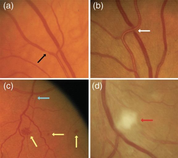
6                                                                                                     Fhima J. et al.

Fig. 3. Border computation process of a vascular network. (A): Vascular network ya ,
(B): Corresponding computed edge of ya .

(Fig. 3). It is computed using the following formula:

          OVPER = 1e2*\frac {\Sigma _{p \in E} \sqrt {2}*\mathbb {1}_{|\partial _x p| + |\partial _y p| = 0}(p) + \mathbb {1}_{|\partial _x p| + |\partial _y p| \neq 0}(p)}{1444^2}    (2)

where E is set of pixel inside the edge image of the vascular network (Fig. 3)
and x/y represent the horizontal/vertical direction.

Overall area: OVAREA is defined as the surface covered by the segmentation.
In terms of pixels, it could be represented as the ratio of white pixels in the
segmentation to the overall number of pixels. It is computed using the following
formula:
                                                                            OVAREA = 1e2*\frac {\Sigma _{p \in V} \mathbb {1}_{1}(p)}{1444^2}                                           (3)

where V is set of pixel inside the image of the vascular network (Fig. 3).

Endpoints and intersection points: The endpoints are the points at the
end of the vascular network, which means in the skeleton version of the network,
the points which have only one neighbor which belongs to the skeleton. The
intersection points are the points where a blood vessel is divided into more
than one blood vessel, which means in the skeleton version of the network, the
points which have more than two neighbors which belong to the skeleton. Their
automatic detection was done using a filter k of size (3x3) where ki,j = 10 if
i = j, or ki,j = 1 otherwise. The skeleton is then convolved with this filter to
obtain a new image. In this new image, the endpoints will be the pixels with
a value of 11, and the intersection points will be the pixels with a value of 13
or larger (Fig. 4). We can represent the endpoints and the intersection points
according to the following equation:

         END = \{p = (i,j) \in Skeleton | (Skeleton \circledast \begin {pmatrix} 1 & 1 & 1\\ 1 & 10 & 1\\ 1&1&1 \end {pmatrix})[i,j] = 11 \}                                            (4)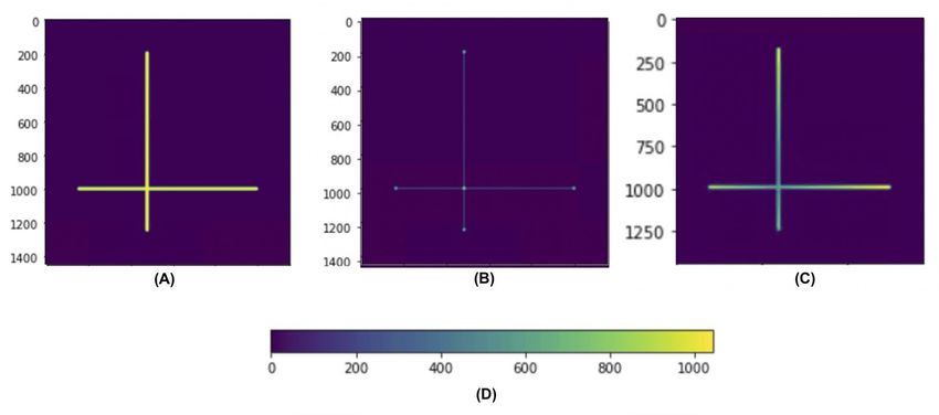
PVBM 7
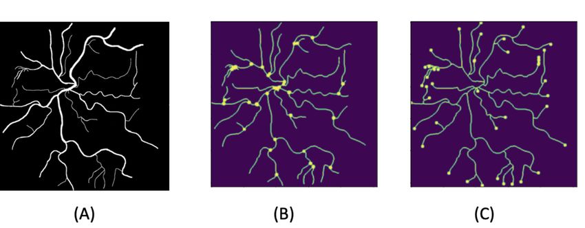
Fig. 4. Automatic detection of the particular points of a vascular network. (A): Vas-
cular network ya , (B): Automatic detection of the intersection points (INTER = 32)
of ya , (C): Automatic detection of the endpoints (END = 40) of ya .
INTER = \{p = (i,j) \in Skeleton | (Skeleton \circledast \begin {pmatrix} 1 & 1 & 1\\ 1 & 10 & 1\\ 1&1&1 \end {pmatrix})[i,j] \geq 13 \} (5)
Particular points is the name given to the combinated set of points resulting
from the union of the endpoints and intersection points. The number of endpoints
(END) and the number of intersection points (INTER) were computed as VBMs.
Median tortuosity: The simplest mathematical method to estimate tortuos-
ity is the arc-chord ratio, defined as the ratio between the length of the curve
and the distance between its ends [19]. In our work, the median tortuosity was
computed using the arc-chord ratio based on the linear interpolation of all the
blood vessels. For that purpose, the skeleton is treated as a graph and particular
points are extracted. To compute the linear interpolation it is then required to
find all the particular points connected to a given particular point. The con-
nection between each particular point was stored in a dictionary according to
Algorithm 1; the output of this algorithm is a dictionary where the keys are the
particular points, and the values are the list of the connected particular points.
Having this dictionary, it is possible to generate the linear interpolation between
each connected particular point, as it is shown in Fig. 5. The tortuosity of each
blood vessel can be estimated by computing the ratio between the blood vessel’s
length (yellow curves in Fig. 5) and the length of the interpolation of this blood
vessel (red lines in Fig. 5). The median tortuosity will then be the median value
of the tortuosity of all the blood vessels.
Algorithm 1
program Compute connected pixel dictionary ( S (= skeleton),
P (= particular point list))
initialize an empty dictionary: connected;
initialize an empty dictionary: visited;8 Fhima J. et al.
for (i,j) in P:
if S[i,j] == 1 (White):
recursive(i,j,S,i,j,visited,P,connected);
end.
program recursive(i_or, j_or, S (= skeleton),
i,j,visited, P(= particular point list) ,connected )
up = (i-1,j);
down = (i+1,j);
left = (i,j-1);
right = (i,j+1);
up left = (i-1,j-1);
up right = (i-1,j+1);
down left = (i+1,j-1);
down right = (i+1,j+1);
if up[0] >= 0 and visited.get(up,default = 0) == 0:
if up not in P:
visited[up] = 1;
if S[up[0]][up[1]] == 1 (White):
point = up;
if point is in P:
connected[i_or,j_or] =
connected.get((i_or,j_or),default = []) + [up];
else:
recursive(i_or, j_or, S, point[0],
point[1],visited,P ,connected);
Do equivalent things for down, left, right, up left, up right,
down left, down right.
end.
Branching angles: A vascular network’s branching angles (BA) can be defined
as the angle where a blood vessel is divided into smaller blood vessels. The
computation of BA is performed using the following steps: starting by extracting
all the angles of a vascular network using a simple modification of the linear
interpolation algorithm that we developed to compute the tortuosity (Fig. 6).
To extract only the branching angles, all other angles need to be discarded.
For instance, in Fig. 6 an ellipse has been drawn around a branching angle,
giving us the following four points A, B, C and D. These points define the
following two segments: [A, C] and [B, D] with their intersection point C. Three
different angles can be computed from this branching: ACD,
\ ACB \ and BCD. \
The branching angle corresponds to ACB.
\ We need to define the centroid of thePVBM 9
Fig. 5. Computing the linear interpolation of a vascular network. (A): Vascular network
ya and (B): Linear interpolation between all the particular points of ya .
graph in order to find the only relevant angle.
In a connected graph, we define a centroid as the closest point to any other
particular point of the graph. To compute the centroid, we will need to extract
a set of points S, which will be our particular points in a connected graph;
S = \{p, p \in skeleton, N(p) \not \in \{2,0\}\} (6)
where N (p) is the number of neighbouring pixels of p which belong to the skele-
ton.
Then we create a metric f such that for any point p in the skeleton of the
segmentation:
f(p)=max_{s \in skeleton} dist(p,s) (7)
where dist is the distance, measured as the number of pixels required to reach s
from p by staying inside the skeleton. The centroid will naturally be the point
with the lowest value according to this function. And for a random point p, the
higher the value of f (p), the farther p is from the centroid. A simple example
can be seen in Fig. 7. This also generalizes to segmentation with multiple dis-
connected parts, assuming that each part has a centroid. The branching angle
between A, B, C, and D is the angle between the 3 points that are the farthest
from the centroid of the blood vessel in terms of pixel distance when you navigate
through the graph of the vascular network which is equivalent to our challenge
of deleting the closest point to the centroid of the blood vessel. It is possible to
delete the irrelevant point thanks to this centroid detection, and to compute the
set of the branching angles Γ = {BAi }i=1:n automatically (Figure 8). The BA
biomarker is defined by the median of all the found angles.
BA = median\{a \in \Gamma \} (8)
where Γ is the set of the detected branching angles.
Fractal dimensions: The retinal blood vessels form a complex branching pat-
tern that can be quantified using fractal dimension (monofractal) [31,30,11]. In10 Fhima J. et al.
Fig. 6. Computation of all the angle of a vascular network.
Fig. 7. Computation of the centroid of a simple graph. (A): Original graph, (B): Par-
ticular point detection, (C) Value of the f (.) function for each pixel of this graph,
(D): Heatmap where the centroid is the point with the lowest value according to the
function f (.).
Fig. 8. Automated computation of the branching angles of the vascular network. (A):
Original segmentation, (B): Branching angles detected automatically.
fractal geometry, the fractal dimension is a measure of the space-filling capacity
of a pattern that tells how a fractal scales differently from the space it is em-PVBM 11
bedded in. Fractal dimension can be thought of as an extension of the familiar
Euclidean dimensions allowing intermediate states. The fractal dimension of the
retinal vascular tree lies between 1 and 2, indicating that its branching pattern
fills space more thoroughly than a line, but less than a plane [30]. The fractal
dimension measures the global branching complexity, which can be altered by
the vessel rarefaction, proliferation and other anatomical changes in a patholog-
ical scenario. The simplest and most common method used in the literature for
monofractal calculation is the box-counting method [31].
However, a single monofractal is limited in describing human eye retinal vas-
culature. It has been observed that retinal vasculature has multifractal properties
which are a generalized notion of a fractal dimension [46,47,48]. Multifractal di-
mensions are characterized by a hierarchy of exponents which can reveal more
complex geometrical properties in a structure [47]. The most common multifrac-
tal dimensions for measuring retinal vasculature are D0 , D1 , D2 which satisfy
the inequality D0 > D1 > D2 [46,39] and also called the capacity dimension
(a monofractal), entropy dimension and correlation dimension respectively. Fol-
lowing [49], we have implemented D0 , D1 , D2 and Singularity length in a similar
manner to Chhabra et al. [7] and the commonly used plugin FracLac [20] for
ImageJ software [41]. The generalized multifractal dimensions are defined as:
\label {dq} D_{q}=\begin {cases} -\lim _{\epsilon \rightarrow 1}\frac {\sum _{i}P_{i}\left (\epsilon \right )\log P_{i}\left (\epsilon \right )}{\log \epsilon } & ,q=1\\\\ \frac {1}{q-1}\lim _{\epsilon \rightarrow 0}\frac {\log \sum _{i}P_{i}^{q}\left (\epsilon \right )}{\log \epsilon } & o.w. \end {cases} (9)
where Pi (ϵ) is the pixel probability in the ith grid box sized ϵ, and q is the order
of the moment of the measure. In addition, multifractals can be described by a
singularity spectrum f (α) − α which is related to the Dq − q spectrum by the
Legendre transformation. In order to calculate f (α) − α spectrum, we use an
alternative approach described by [7]:
\label {fq} f\left (q\right ) =\lim _{\epsilon \rightarrow 0}\frac {\sum _{i}\mu _{i}\left (q,\epsilon \right )\log \mu _{i}\left (q,\epsilon \right )}{\log \epsilon } (10)
\label {aq} \alpha \left (q\right ) =\lim _{\epsilon \rightarrow 0}\frac {\sum _{i}\mu _{i}\left (q,\epsilon \right )\log P_{i}\left (\epsilon \right )}{\log \epsilon } (11)
\mu _{i}\left (q,\epsilon \right ) =\frac {P_{i}\left (\epsilon \right )^{q}}{\sum _{i}P_{i}\left (\epsilon \right )^{q}} (12)
The f (α) − α spectrum is characterized by a bell shaped curve with one maxima
point. From this curve, an additional biomarker is computed - the spectrum range
∆α which is also called Singularity Length (SL).
\alpha _{\text {min}}=\lim _{q\rightarrow \infty }\alpha \left (q\right ),\:\alpha _{\text {max}}=\lim _{q\rightarrow -\infty }\alpha \left (q\right ) (13)
\Delta \alpha =\alpha _{\text {max}}-\alpha _{\text {min}} (14)12 Fhima J. et al.
SL quantifies the multifractality degree [29] of an image.
The calculation of equations 9, 10, 11 was done by linear regression with a
linear set of box sizes ϵ for every q. The values of these graphs are sensitive to grid
placement on the segmented DFI image, as they depend on pixel distribution
across the image. We followed a similar optimization method as used by the
FracLac plugin [20], which is to change the sampling grid location by rotating the
image randomly, and to choose the measurement which satisfies the inequality
D0 > D1 > D2 and has the highest value of D0 . In addition, to overcome
numerical issues saturated grid boxes and grid boxes with low occupancy of
pixels were ignored. αmin and αmax were estimated by αmin ≈ α (q = 10) and
αmax ≈ α (q = −10).
Benchmark against existing software: In order to validate the implementa-
tion of some of the biomarkers we implemented in PVBM we benchmarked their
values against two ImageJ plugins, namely AnalyzeSkeleton [2] and FracLac [20].
The benchmark was performed for the arterioles from the entire UZFG dataset.
A direct benchmark could be performed for the following biomarkers: OVAREA,
TOR, D0 , D1 , D2 and SL. An extrapolated comparison could be performed for
the OVLEN. Indeed, these were not directly outputted by the plugin, but could
be derived from the AnalyzeSkeleton [2] plugin. No benchmark could be per-
formed for OVPER, END, INTER and BA because of the lack of open source
available benchmark software.
3 Results
Table 3 shows that the VBMs benchmarked against reference software had very
close values with normalized root mean square errors ranging from 0 to 0.316.
Table 4 and 5 provide summary statistics and a statistical analysis of the
VBMs for the GLA NOR groups. The statistics were presented as median and
interquartile (Q1 and Q3), and the p-value from the Wilcoxon signed-rank. The
arteriolar OVAREA, OVLEN, and END were the most significant in distinguish-
ing between the two groups. Fig. 9 presents qualitative examples of three DFIs
with arteriolar OVAREA, OVLEN, BA, END and D0 VBM values.
4 Discussion and future work
The first contribution of this work is the creation of a toolbox for VBMs, which
is made open source under a GNU GPL 3 license and will be made available
on physiozoo.com (following publication). In particular, novel algorithms were
introduced to estimate the tortuosity and branching angles.
The second contribution of this work is the application of the PVBM tool-
box to a new dataset of manually segmented vessels from DFIs. The statistical
analysis that we have performed showed that the arterioles-based biomarkers are
the most significant in distinguishing between NOR and GLA. For arterioles andPVBM 13
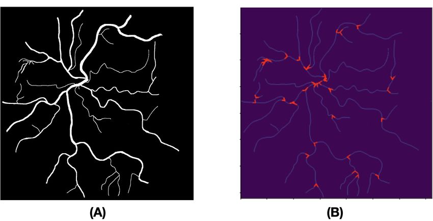
Fig. 9. Example of biomarkers computed from the arterioles of two DFIs. The first row
is a DFI of a healthy control (NOR) and the second column is from a glaucoma patient
(GLA). The OVAREA biomarker shows a larger vascular area in the NOR images.
The BA biomarker shows that the branching of the NOR image are bigger than the
one of the GLA image. Finally, the END biomarker indicates that the GLA image had
less arteriolar branching compared to healthy controls, leading to a lower number of
endpoints.
venules, all biomarkers were significant and lower in glaucoma patients compared
to healthy controls except for tortuosity, venular singularity length and venular
branching angles.
A limitation of our experiment is that although the images were taken with
the same procedure, which includes the disk being centered, there is some vari-
ation in the exact location of the disk due to the non-automated operation. In
future work, we need to consider the detection of the disk to delineate a circular
frame centered on the disk to engineer the vasculature biomarkers more consis-
tently. Furthermore, other biomarkers may be implemented such as the vessel
Table 3. PVBM benchmark against reference ImageJ plugins using the arterioles of
the UZFG dataset. µ: mean, σ: standard deviation, RMSE: root mean square error,
NRMSE: normalized root mean square error.
Biomarker Benchmark Benchmark This work Difference
results
µ σ µ σ RMSE NRMSE
OVLEN AnalyzeSkeleton [2] 4.687 0.928 4.868 0.974 0.194 0.060
OVAREA ImageJ [41] 4.939 0.011 4.939 0.011 0 0
TOR AnalyzeSkeleton [2] 1.081 0.007 1.084 0.007 0.003 0.11
D0 FracLac [20] 1.373 0.035 1.425 0.026 0.054 0.301
D1 FracLac [20] 1.367 0.034 1.390 0.027 0.028 0.155
D2 FracLac [20] 1.361 0.033 1.375 0.028 0.021 0.115
SL FracLac [20] 0.626 0.104 0.645 0.076 0.128 0.31614 Fhima J. et al.
Table 4. Summary of the biomarkers analyzed for arterioles (a ) and extracted with
the PVBM toolbox with their median (Q1-Q3). Refer to Table 2 for the definition of
the VBM acronyms. P-values are provided using the Wilcoxon signed-rank test.
NOR (n=19) GLA (n=50) p
OVAREAa 5.82 (5.26-6.23) 4.52 (3.76-5.44) 4e-4
OVLENa 5.53 (5.28-6.21) 4.85 (4.33-5.37) 1e-4
OVPERa 3.94 (3.74-4.33) 3.44 (3.01-3.80) 2e-4
BAa 87.29 (81.88-93.28) 81.93 (75.41-87.87) 2e-2
ENDa 37.0 (28.5-43.5) 27.0 (21.0-32.75) 7e-4
INTERa 36.0 (28.5-43.0) 24.5 (20.0-30.0) 8e-4
TORa 1.08 (1.08-1.09) 1.08(1.08-1.09) 1e − 1
D0a 1.44 (1.42-1.45) 1.42 (1.40-1.44) 5e-3
D1a 1.41 (1.38-1.42) 1.38 (1.37-1.40) 3e-3
D2a 1.39 (1.37-1.40) 1.37 (1.35-1.38) 4e-3
SLa 0.62 (0.59-0.64) 0.64 (0.62-0.78) 9e-3
Table 5. Summary of the biomarkers analyzed for venules (v ) and extracted with the
PVBM toolbox with their median (Q1-Q3). Refer to Table 2 for the definition of the
VBM acronyms. P-values are provided using the Wilcoxon signed-rank test.
NOR (n=19) GLA (n=50) p
OVAREAv 6.3 (5.82-6.71) 5.28 (4.59-6.01) 9e-4
OVLENv 5.42 (4.82-5.67) 4.69 (4.21-5.13) 1e-3
OVPERv 3.77 (3.36-3.99) 3.26 (2.96-3.59) 3e-3
BAv 84.14 (78.74-86.9) 85.1 (81.52-91.08) 1e − 1
ENDv 339.0 (31.5-43.0) 28.5 (23.0-34.0) 1e-3
INTERv 36.0 (31.5-42.5) 27.0 (21.0-33.0) 1e-3
TORv 1.08 (1.08-1.09) 1.08 (1.08-1.09) 4e − 1
D0v 1.43 (1.4-1.44) 1.40 (1.38-1.42) 4e-3
D1v 1.38 (1.36-1.40) 1.37 (1.35-1.38) 8e-3
D2v 1.36 (1.34-1.39) 1.35 (1.33-1.36) 1e-2
SLv 0.61 (0.58-0.66) 0.63 (0.59-0.66) 2e − 1
diameter [13], CRAE [37], CRVE [37], branching coefficients [10] which is the
ratio of the sum of the cross-sectional areas of the two daughter vessels to the
cross-sectional area of the parent vessel at an arteriolar bifurcation [10]. Finally,
it is to be studied to what extent VBMs may be evaluated from vasculature
obtained using an automated (versus manual) segmentation algorithm as well as
the effect of DFI quality [1] on the results.PVBM 15
References
1. Abramovich, O., Pizem, H., Van Eijgen, J., Stalmans, I., Blumenthal, E., Behar,
J.: FundusQ-Net: a Regression Quality Assessment Deep Learning Algorithm for
Fundus Images Quality Grading. arXiv preprint arXiv:2205.01676 (2022)
2. Arganda-Carreras, I., Fernández-González, R., Muñoz-Barrutia, A., Ortiz-De-
Solorzano, C.: 3D reconstruction of histological sections: Application to mammary
gland tissue. Microscopy research and technique 73(11), 1019–1029 (2010)
3. Badawi, S.A., Fraz, M.M.: Multiloss function based deep convolutional neural net-
work for segmentation of retinal vasculature into arterioles and venules. BioMed
research international 2019 (2019)
4. Betzler, B.K., Sabanayagam, C., Tham, Y., Cheung, C.Y., Cheng, C., Wong, T.,
Nusinovici, S.: Retinal Vascular Profile in Predicting Incident Cardiometabolic
Diseases among Individuals with Diabetes. Microcirculation p. e12772 (2022)
5. Brinchmann-Hansen, O., Heier, H.: Theoretical relations between light streak
characteristics and optical properties of retinal vessels. Acta Ophthalmologica
64(S179), 33–37 (1986)
6. Cheung, N., Donaghue, K.C., Liew, G., Rogers, S.L., Wang, J.J., Lim, S.W., Jenk-
ins, A.J., Hsu, W., Lee, M.L., Wong, T.Y.: Quantitative assessment of early dia-
betic retinopathy using fractal analysis. Diabetes care 32(1), 106–110 (2009)
7. Chhabra, A., Jensen, R.V.: Direct determination of the f (α) singularity spectrum.
Physical Review Letters 62(12), 1327 (1989)
8. Dashtbozorg, B., Mendonca, A.M., Penas, S., Campilho, A.: RetinaCAD, a system
for the assessment of retinal vascular changes. In: 2014 36th Annual International
Conference of the IEEE Engineering in Medicine and Biology Society. pp. 6328–
6331. IEEE (2014)
9. Doubal, F.N., MacGillivray, T.J., Patton, N., Dhillon, B., Dennis, M.S., Wardlaw,
J.M.: Fractal analysis of retinal vessels suggests that a distinct vasculopathy causes
lacunar stroke. Neurology 74(14), 1102–1107 (2010)
10. Doubal, F.N., De Haan, R., MacGillivray, T.J., Cohn-Hokke, P.E., Dhillon, B.,
Dennis, M.S., Wardlaw, J.M.: Retinal arteriolar geometry is associated with cere-
bral white matter hyperintensities on magnetic resonance imaging. International
Journal of Stroke 5(6), 434–439 (2010)
11. Family, F., Masters, B.R., Platt, D.E.: Fractal pattern formation in human retinal
vessels. Physica D: Nonlinear Phenomena 38(1-3), 98–103 (1989)
12. Fhima, J., Van Eijgen, J., Freiman, M., Stalmans, I., Behar, J.A.: Lirot.ai: A
Novel Platform for Crowd-Sourcing Retinal Image Segmentations. In: Accepted
for proceeding in Computing in Cardiology 2022 (2022)
13. Goldenberg, D., Shahar, J., Loewenstein, A., Goldstein, M.: Diameters of retinal
blood vessels in a healthy cohort as measured by spectral domain optical coherence
tomography. Retina 33(9), 1888–1894 (2013)
14. Grisan, E., Foracchia, M., Ruggeri, A.: A Novel Method for the Automatic Grading
of Retinal Vessel Tortuosity. IEEE Transactions on Medical Imaging 27(3), 310–
319 (2008)
15. Gunn, R.M.: Ophthalmoscopic evidence of (1) arterial changes associated with
chronic renal disease, and (2) of increased arterial tension. Transactions of the
Ophthalmological Society of the United Kingdom 12, 124–125 (1892)
16. Gunn, R.M.: Ophthalmoscopic evidence of general arterial disease. Trans Ophthal-
mol Soc UK 18, 356–381 (1898)16 Fhima J. et al.
17. Guo, S., Yin, S., Tse, G., Li, G., Su, L., Liu, T.: Association between caliber of
retinal vessels and cardiovascular disease: a systematic review and meta-analysis.
Current Atherosclerosis Reports 22(4), 1–13 (2020)
18. Hanssen, H., Nickel, T., Drexel, V., Hertel, G., Emslander, I., Sisic, Z., Lorang,
D., Schuster, T., Kotliar, K.E., Pressler, A.: Exercise-induced alterations of reti-
nal vessel diameters and cardiovascular risk reduction in obesity. Atherosclerosis
216(2), 433–439 (2011)
19. Hart, W.E., Goldbaum, M., Côté, B., Kube, P., Nelson, M.R.: Measurement and
classification of retinal vascular tortuosity. International Journal of Medical Infor-
matics 53(2), 239–252 (1999)
20. Karperien, A.: Fraclac for imagej (2013)
21. Kaushik, S., Tan, A.G., Mitchell, P., Wang, J.J.: Prevalence and associations of
enhanced retinal arteriolar light reflex: a new look at an old sign. Ophthalmology
114(1), 113–120 (2007)
22. Kawasaki, R., Wang, J.J., Rochtchina, E., Lee, A.J., Wong, T.Y., Mitchell, P.:
Retinal vessel caliber is associated with the 10-year incidence of glaucoma: the
Blue Mountains Eye Study. Ophthalmology 120(1), 84–90 (2013)
23. Keith, N.M.: Some differente types of essential hypertension: their course and prog-
nosis. Am J Med Sci 197, 332–343 (1939)
24. Lemmens, S., Luyts, M., Gerrits, N., Ivanova, A., Landtmeeters, C., Peeters, R.,
Simons, A., Vercauteren, J., Sunaric-Mégevand, G., Van Keer, K.: Age-related
changes in the fractal dimension of the retinal microvasculature, effects of cardio-
vascular risk factors and smoking behaviour. Acta Ophthalmologica (2021)
25. Liew, G., Mitchell, P., Rochtchina, E., Wong, T.Y., Hsu, W., Lee, M.L., Wain-
wright, A., Wang, J.J.: Fractal analysis of retinal microvasculature and coronary
heart disease mortality. European heart journal 32(4), 422–429 (2011)
26. Liew, G., Wang, J.J.: Retinal vascular signs: a window to the heart? Revista Es-
pañola de Cardiología (English Edition) 64(6), 515–521 (2011)
27. Liew, G., Wang, J.J., Cheung, N., Zhang, Y.P., Hsu, W., Lee, M.L., Mitchell, P.,
Tikellis, G., Taylor, B., Wong, T.Y.: The retinal vasculature as a fractal: methodol-
ogy, reliability, and relationship to blood pressure. Ophthalmology 115(11), 1951–
1956 (2008)
28. Lotmar, W., Freiburghaus, A., Bracher, D.: Measurement of vessel tortuosity on
fundus photographs. Albrecht von Graefes Archiv für klinische und experimentelle
Ophthalmologie 211(1), 49–57 (1979)
29. Macek, W.M., Wawrzaszek, A.: Evolution of asymmetric multifractal scaling of
solar wind turbulence in the outer heliosphere. Journal of Geophysical Research:
Space Physics 114(A3) (2009)
30. Mainster, M.A.: The fractal properties of retinal vessels: embryological and clinical
implications. Eye 4(1), 235–241 (1990)
31. Mandelbrot, B.B., Mandelbrot, B.B.: The fractal geometry of nature, vol. 1. WH
freeman New York (1982)
32. Martínez-Pérez, M.E., Hughes, A.D., Stanton, A.V., Thom, S.A., Chapman, N.,
Bharath, A.A., Parker, K.H.: Geometrical and Morphological Analysis of Vascular
Branches from Fundus Retinal Images. In: Delp, S.L., DiGoia, A.M., Jaramaz, B.
(eds.) Medical Image Computing and Computer-Assisted Intervention – MICCAI
2000. pp. 756–765. Springer Berlin Heidelberg, Berlin, Heidelberg (2000)
33. Mehta, R., Ying, G.S., Houston, S., Isakova, T., Nessel, L., Ojo, A., Go, A., Lash, J.,
Kusek, J., Grunwald, J.: Phosphate, fibroblast growth factor 23 and retinopathy in
chronic kidney disease: the Chronic Renal Insufficiency Cohort Study. Nephrology
Dialysis Transplantation 30(9), 1534–1541 (2015)PVBM 17
34. Miri, M., Amini, Z., Rabbani, H., Kafieh, R.: A comprehensive study of retinal ves-
sel classification methods in fundus images. Journal of medical signals and sensors
7(2), 59 (2017)
35. Murphy, S.L., Kochanek, K.D., Xu, J., Arias, E.: Mortality in the United States,
2020 (2021)
36. Owen, C.G., Rudnicka, A.R., Mullen, R., Barman, S.A., Monekosso, D., Whincup,
P.H., Ng, J., Paterson, C.: Measuring retinal vessel tortuosity in 10-year-old chil-
dren: validation of the computer-assisted image analysis of the retina (CAIAR)
program. Investigative ophthalmology & visual science 50(5), 2004–2010 (2009)
37. Parr, J.C., Spears, G.F.S.: General caliber of the retinal arteries expressed as the
equivalent width of the central retinal artery. American journal of ophthalmology
77(4), 472–477 (1974)
38. Perez-Rovira, A., MacGillivray, T., Trucco, E., Chin, K.S., Zutis, K., Lupascu, C.,
Tegolo, D., Giachetti, A., Wilson, P.J., Doney, A.: VAMPIRE: vessel assessment
and measurement platform for images of the REtina. In: 2011 Annual International
Conference of the IEEE Engineering in Medicine and Biology Society. pp. 3391–
3394. IEEE (2011)
39. Posadas, A.N.D., Giménez, D., Bittelli, M., Vaz, C.M.P., Flury, M.: Multifractal
characterization of soil particle-size distributions. Soil Science Society of America
Journal 65(5), 1361–1367 (2001)
40. Provost, E.B., Nawrot, T.S., Int Panis, L., Standaert, A., Saenen, N.D., De Boever,
P.: Denser Retinal Microvascular Network Is Inversely Associated With Behavioral
Outcomes and Sustained Attention in Children. Frontiers in neurology 12, 547033
(2021)
41. Rasband, W.S.: Imagej, us national institutes of health, bethesda, maryland, usa
(2011)
42. Sabanayagam, C., Shankar, A., Koh, D., Chia, K.S., Saw, S.M., Lim, S.C., Tai,
E.S., Wong, T.Y.: Retinal microvascular caliber and chronic kidney disease in an
Asian population. American journal of epidemiology 169(5), 625–632 (2009)
43. Scheie, H.G.: Evaluation of ophthalmoscopic changes of hypertension and arteriolar
sclerosis. AMA archives of ophthalmology 49(2), 117–138 (1953)
44. Sharrett, A.R., Hubbard, L.D., Cooper, L.S., Sorlie, P.D., Brothers, R.J., Nieto,
F.J., Pinsky, J.L., Klein, R.: Retinal arteriolar diameters and elevated blood pres-
sure: the Atherosclerosis Risk in Communities Study. American journal of epidemi-
ology 150(3), 263–270 (1999)
45. Sng, C.C.A., Sabanayagam, C., Lamoureux, E.L., Liu, E., Lim, S.C., Hamzah,
H., Lee, J., Tai, E.S., Wong, T.Y.: Fractal analysis of the retinal vasculature
and chronic kidney disease. Nephrology Dialysis Transplantation 25(7), 2252–2258
(2010)
46. Stosic, T., Stosic, B.D.: Multifractal analysis of human retinal vessels. IEEE trans-
actions on medical imaging 25(8), 1101–1107 (2006)
47. Ţălu, Ş.: Characterization of retinal vessel networks in human retinal imagery using
quantitative descriptors. Human and Veterinary Medicine 5(2), 52–57 (2013)
48. Ţălu, Ş., Stach, S., Călugăru, D.M., Lupaşcu, C.A., Nicoară, S.D.: Analysis of
normal human retinal vascular network architecture using multifractal geometry.
International journal of ophthalmology 10(3), 434 (2017)
49. Van Craenendonck, T., Gerrits, N., Buelens, B., Petropoulos, I.N., Shuaib, A.,
Standaert, A., Malik, R.A., De Boever, P.: Retinal microvascular complexity com-
paring mono-and multifractal dimensions in relation to cardiometabolic risk factors
in a Middle Eastern population. Acta Ophthalmologica 99(3), e368–e377 (2021)18 Fhima J. et al.
50. Witt, N., Wong, T.Y., Hughes, A.D., Chaturvedi, N., Klein, B.E., Evans, R., McNa-
mara, M., Thom, S.A.M., Klein, R.: Abnormalities of retinal microvascular struc-
ture and risk of mortality from ischemic heart disease and stroke. Hypertension
47(5), 975–981 (2006)You can also read