Progress in Oceanography - Contents lists available at ScienceDirect - NERC Open Research ...
←
→
Page content transcription
If your browser does not render page correctly, please read the page content below
Progress in Oceanography 197 (2021) 102653
Contents lists available at ScienceDirect
Progress in Oceanography
journal homepage: www.elsevier.com/locate/pocean
Environment, ecology, and potential effectiveness of an area protected from
deep-sea mining (Clarion Clipperton Zone, abyssal Pacific)
Daniel O.B. Jones a, *, Erik Simon-Lledó a, Diva J. Amon b, Brian J. Bett a, Clémence Caulle c,
Louis Clément a, Douglas P. Connelly a, Thomas G. Dahlgren d, e, Jennifer M. Durden a,
Jeffrey C. Drazen f, Janine Felden g, Andrew R. Gates a, Magdalena N. Georgieva b,
Adrian G. Glover b, Andrew J. Gooday a, b, Anita L. Hollingsworth a, h, Tammy Horton a,
Rachael H. James h, Rachel M. Jeffreys i, Claire Laguionie-Marchais j, Astrid B. Leitner k,
Anna Lichtschlag a, Amaya Menendez h, Gordon L.J. Paterson b, Kate Peel a, Katleen Robert l,
Timm Schoening m, Natalia A. Shulga n, Craig R. Smith f, Sergio Taboada b, o, p,
Andreas M. Thurnherr q, Helena Wiklund b, e, C. Robert Young a, Veerle A.I. Huvenne a
a
National Oceanography Centre, European Way, Southampton SO14 3ZH, UK
b
Life Sciences Department, Natural History Museum, Cromwell Rd, London SW7 5BD, UK
c
Ocean Zoom, Nantes 44200 / Brest 29200, France
d
NORCE, Postboks 22 Nygårdstangen, 5838 Bergen, Norway
e
Gothenburg Global Biodiversity Centre and Department of Marine Sciences, University of Gothenburg, 40530 Gothenburg, Sweden
f
University of Hawai’i at Manoa, Department of Oceanography, 1000 Pope Rd, Honolulu, HI 96821, USA
g
MARUM – Center for Marine Environmental Sciences, University of Bremen, Leobener Str. 8, D-28359 Bremen, Germany
h
Ocean and Earth Science, University of Southampton, National Oceanography Centre Southampton, University of Southampton Waterfront Campus, European Way,
Southampton SO14 3ZH, UK
i
School of Environmental Sciences, University of Liverpool, Liverpool, UK
j
Ryan Institute, & School of Natural Sciences, Zoology, NUI Galway, University Road, Galway, Ireland
k
Monterey Bay Aquarium Research Institute, 7700 Sandholdt Rd, Moss Landing, CA 95039, USA
l
Fisheries and Marine Institute of Memorial University of Newfoundland, Canada
m
Deep Sea Monitoring Group, GEOMAR Helmholtz Center for Ocean Research, Kiel, Germany
n
Shirshov Institute of Oceanology, Russian Academy of Sciences, Moscow, Russia
o
Departamento de Biodiversidad, Ecología y Evolución, Universidad Complutense de Madrid, Madrid, Spain
p
Departamento de Ciencias de la Vida, Universidad de Alcalá de Henares, Madrid, Spain
q
Lamont-Doherty Earth Observatory, Palisades, NY, 10964-8000, USA
A R T I C L E I N F O A B S T R A C T
Keywords: To protect the range of habitats, species, and ecosystem functions in the Clarion Clipperton Zone (CCZ), a region
Area of Particular Environmental Interest of interest for deep-sea polymetallic nodule mining in the Pacific, nine Areas of Particular Environmental Interest
APEI-6 (APEIs) have been designated by the International Seabed Authority (ISA). The APEIs are remote, rarely visited
Environmental Management
and poorly understood. Here we present and synthesise all available observations made at APEI-6, the most north
Baseline
Clarion-Clipperton Zone
eastern APEI in the network, and assess its representativity of mining contract areas in the eastern CCZ. The two
Polymetallic nodules studied regions of APEI-6 have a variable morphology, typical of the CCZ, with hills, plains and occasional
Ocean conservation seamounts. The seafloor is predominantly covered by fine-grained sediments, and includes small but abundant
Marine protected area polymetallic nodules, as well as exposed bedrock. The oceanographic parameters investigated appear broadly
similar across the region although some differences in deep-water mass separation were evident between APEI-6
and some contract areas. Sediment biogeochemistry is broadly similar across the area in the parameters inves
tigated, except for oxygen penetration depth, which reached >2 m at the study sites within APEI-6, deeper than
that found at UK1 and GSR contract areas. The ecology of study sites in APEI-6 differs from that reported from
UK1 and TOML-D contract areas, with differences in community composition of microbes, macrofauna, xen
ophyophores and metazoan megafauna. Some species were shared between areas although connectivity appears
* Corresponding author.
E-mail address: dj1@noc.ac.uk (D.O.B. Jones).
https://doi.org/10.1016/j.pocean.2021.102653
Received 28 January 2021; Received in revised form 17 June 2021; Accepted 14 July 2021
Available online 21 July 2021
0079-6611/© 2021 The Authors. Published by Elsevier Ltd. This is an open access article under the CC BY license (http://creativecommons.org/licenses/by/4.0/).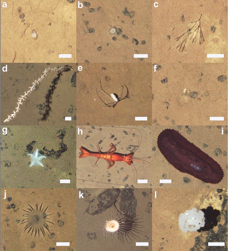
D.O.B. Jones et al. Progress in Oceanography 197 (2021) 102653
limited. We show that, from the available information, APEI-6 is partially representative of the exploration areas
to the south yet is distinctly different in several key characteristics. As a result, additional APEIs may be war
ranted and caution may need to be taken in relying on the APEI network alone for conservation, with other
management activities required to help mitigate the impacts of mining in the CCZ.
1. Introduction Here, we collate these data to provide an overview of two sampled lo
calities in the easternmost of the CCZ APEIs, APEI-6, to initiate a base
The Clarion-Clipperton Zone (CCZ) is a seabed area of approximately line description of the geological, physical, chemical and biological
6 million km2, receiving scientific and commercial interest for its vast conditions on and near the seabed. Although the information presented
resources of polymetallic nodules (Lodge et al., 2014). The CCZ is situ here is far from complete, it provides a valuable insight into what is
ated in the eastern Pacific between the Clarion and Clipperton fracture currently one of the best studied APEIs. The localities investigated in
zones stretching from 5◦ to 20◦ N and 115 to 160◦ W and covers over 1% APEI-6 are then compared with sites in adjacent exploration areas to
of the world’s surface. There has been a long history of scientific and help provide an initial assessment of how representative these APEI sites
industrial exploration of this area. Nodules were first discovered close to are of areas potentially subject to mining pressure in the eastern CCZ. As
the CCZ by the 1872–1876 HMS Challenger expedition (Murray and well as having scientific interest, such information is of great importance
Renard, 1891). The first studies of potential mining impacts were carried for understanding better the environment and potential impacts of deep-
out here in the 1970s (reviewed in Jones et al., 2017) but commercial sea mining on the environment to ensure effective management and
exploitation has not yet occurred. As the CCZ is predominantly seabed regulation.
beyond national jurisdiction, the mineral resources are regulated by the
International Seabed Authority (ISA). The ISA has divided the CCZ into 2. Methods
various mining exploration contract areas assigned to state-sponsored
contractors. In addition, the ISA has produced a spatial management 2.1. Study areas
plan for the CCZ that includes nine Areas of Particular Environmental
Interest (APEIs), with original locations designed to be areas represen Data were collected from two areas of APEI-6, the southwest (APEI-6
tative of the region expected to sustain mining impacts (Wedding et al., SW) and the northeast (APEI-6 NE; Table 1; Fig. 1; Supplementary
2013). The original design of APEIs was based on modelled information Figure 1). In some cases, comparisons were possible to data collected in
on environmental characteristics, such as food supply based on partic an identical way in the UK1 (United Kingdom-sponsored exploration
ulate organic carbon flux (Smith et al., 2008), nodule density, seabed area 1, contracted to UK Seabed Resources) contract area in the eastern
morphology, together with expert opinion. In addition, the locations of CCZ (Table 1). The majority of the data used in this paper were obtained
existing and emerging exploration contracts were taken into account from APEI-6 SW during the RRS James Cook cruise 120 (JC120) expe
(Wedding et al., 2013). Two of the APEIs were moved by the ISA from dition (Table 1) (Jones et al., 2015) and the methods described below
the central area, with the area now designated as APEI-6 moved to the specifically refer to this dataset, unless stated otherwise. Additional data
northeast corner of the CCZ (Wedding et al., 2013). Importantly, so far used in this paper (Table 1) were collected during expeditions AB01
there has been limited scientific research within the APEIs and the (MV1313) (Smith et al., 2013) to UK1 and AB02 (TN319) (Smith et al.,
seafloor ecosystems in several have not been sampled or studied 2015a) to UK1 and APEI-6 NE. A summary of the samples analysed here
(Laroche et al., 2020; Leitner et al., 2017; Simon-Lledó et al., 2019a; is presented in Table 2.
Vanreusel et al., 2016; Washburn et al., 2021). For example, the recent The study area in APEI-6 SW was selected based on global datasets
Friday Harbor workshop (International Seabed Authority, 2020) high (GEBCO, 2014) and initial multibeam data to have a similar topo
lighted the importance of sampling at the APEI sites. graphical relief to that often found in contract areas (e.g. Simon-Lledó
Although the CCZ consists predominantly of abyssal plains, sub et al., 2020). The area of interest was set within a 6,300 km2 rectangle of
stantial environmental and biological variation is apparent (Washburn seafloor, approximately 20 nautical miles away from the southwestern
et al., 2021). This broad-scale heterogeneity is also apparent in existing corner of APEI-6. A much smaller area (380 km2) was surveyed in the
data within the APEI system. In APEI-6, the shallowest of the APEIs northeastern corner of APEI-6 during the TN319 (AB02) expedition
(based on mean depth), the seabed landscape is comprised of elongated (Table 1). Water depth within this area ranged between 3900 and 4150
abyssal hills (Simon-Lledó et al., 2019a) with occasional seamounts over m, with a similar geomorphology to APEI-6 SW. APEI-6 NE was studied
1500 m elevation (Washburn et al., 2021). These features co-occur with opportunistically with ship time remaining at the end of cruise TN319
other variations in the geological, chemical and biological environment (AB02) during transit from the UK1 license area to the final port of San
(Leitner et al., 2017). At a finer scale, variations in resource supply Diego.
create patches of organic enrichment that may enhance biological het Even the area mapped with multibeam (total of 6,680 km2) at APEI-6
erogeneity (Smith et al., 1996). only represents a small percentage (4%) of the total area of APEI-6
Even at the regional scale, there are relatively few studies on biology (including central and buffer areas: 400 × 400 km). Undoubtedly,
of the CCZ and the distributions of species (Taboada et al., 2018). It has much of the variation found across all of APEI-6 is missed. Furthermore,
been hypothesised that benthic species with widespread distributions some of the sample sizes in the datasets (Table 2) are small and unsuited
(Drazen et al., 2021; Glover et al., 2002) exist alongside a high diversity to quantitative analysis or robust comparisons. These have been clearly
of rare species (Smith et al., 2008; Smith, et al., 2019). Large numbers of indicated. Small datasets have been included as they can still provide
species across all size classes in the CCZ have been documented recently, important information for a poorly studied area like APEI-6.
and include regional records of species or morphospecies based on im
agery (Amon et al., 2017a; Amon et al., 2017b), molecular data (Janssen 2.1.1. Mapping
et al., 2015; Janssen et al., 2019), and combined molecular and In APEI-6 SW, multibeam data were collected with a shipboard
morphological evidence (Dahlgren et al., 2016; Glover et al., 2016b; Simrad EM120 system on board the RRS James Cook (191 beams). They
Gooday et al., 2020b; Wiklund et al., 2019; Wiklund et al., 2017). Re were processed using CARIS HIPS and SIPS software (CARIS; v8.0). The
cords from the APEIs specifically were almost absent until recent years. mapping data (50 m pixels) were used to delineate areas for further
A series of recent expeditions have provided new insights into the assessment representing characteristic landscape types: plains, ridges
environment of the CCZ based on a wide range of multidisciplinary data. and troughs (Simon-Lledó et al., 2019a). A seamount, located towards
2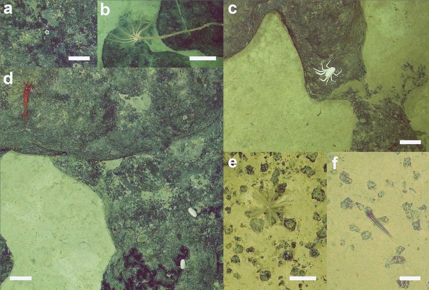
D.O.B. Jones et al. Progress in Oceanography 197 (2021) 102653
the southern end (16◦ 51.94′ N 122◦ 41.27′ W) of the study area (Fig. 1) samples. Observations of microtextures and maps of the distribution of
was also assessed. Multibeam data from APEI-6 NE were collected with a mineral phases and chemical composition were made using Scanning
shipboard Kongsberg EM302 Multibeam Sonar. Data were projected in Electron Microscopy (SEM). More details are available in Menendez
UTM, Zone 10 N, using the World Geodetic System 1984 datum. et al. (2019) and Reykhard and Shulga (2019).
2.1.2. Seafloor sampling 2.3. Sediment properties
A wide range of seabed and water column samples were obtained in
APEI-6 SW (Supplementary Figure 1) following a stratified random 2.3.1. Grain size
sampling design (Simon-Lledó et al., 2019a). Although samples were Five Megacore deployment locations were randomly allocated with a
stratified by topography at APEI-6 SW, we report the combined results of minimum separation of 100 m within the flat, ridge and trough study
these samples here to represent the entire APEI-6 SW survey area. areas and three locations on the deep plain during JC120 at APEI-6 SW.
Opportunistic samples were also obtained in the northern part of UK1. Additionally, one randomly allocated Megacore deployment was also
For parameters that are not explored in more detail in other papers, we obtained from the seamount at APEI-6 SW and the UK1 area during
present data for the stratified areas and UK1 site separately in the sup JC120. Once retrieved, cores were sliced and split into nine different
plementary material. Metadata for all known samples within APEI-6 and sediment depths (0–0.5, 0.5–1, 1–1.5, 1.5–2, 2–3, 3–5, 5–10, 10–15, and
the JC120 samples from UK1 are presented in supplementary Table 1. 15–20 cm below seafloor, cmbf). Sediment grain size of each separate
Sediment samples were obtained by boxcore (United States Naval layer was measured independently by laser diffraction (Malvern Mas
Electronics Laboratory (USNEL) type, 50x50 cm square box), Megacore tersizer; full methods in (Simon-Lledó et al., 2019a)). For subsequent
(Bowers & Connelly design; 10 cm internal diameter cores) and gravity analyses, mean particle size distribution for each replicate site was
core (3 m long barrel, 70 mm internal diameter core liner). Faunal computed for combined 0–5, 5–10, 10–15, and 15–20 cmbf horizons.
samples were obtained by Agassiz trawl (3 m width, 10 mm mesh size),
epibenthic sled (Brenke, 2005), baited traps (Horton et al., 2020b), and 2.3.2. Sediment pore water geochemistry
opportunistic collections from other samplers. Sediments at APEI-6 SW and UK1 were obtained with a 3 m-long
Gravity corer (GC) and with a Megacorer that collected the upper ~ 0.4
2.1.3. Water column sampling m of the seafloor sediments. Immediately after retrieval, the GCs were
Several CTD (Conductivity Temperature Depth) profiles were sectioned in 0.5 m intervals, oxygen concentrations measured using
collected with a SBE 911plus CTD in APEI-6 SW on JC120. The UK1 site needle-type fiber-optical oxygen microsensors (OXR50-OI, PyroS
was sampled during JC120 and the ABYSSLINE cruises AB01 (MV1313, cience©) and porewater extracted with Rhizons (Rhizon CSS: length 5
October 2013; (Smith et al., 2013)) and AB02 (TN319, February 2015; cm, pore diameter 0.2 µm; Rhizosphere Research Products, Wageningen,
(Smith et al., 2015a)). The accuracy of the salinity and the oxygen Netherlands) inserted though pre-drilled holes in the GC liners. The
measurements from all these cruises are expected to be within ± 0.003 g same intervals were collected for each GC section, 5, 15, 25, 35 and 45
kg− 1 and ± 0.05 mL L-1, respectively. We use the TEOS-10 equation of cm. Aliquots of porewater were collected for cations, nitrate and Total
state (McDougall et al., 2010) to derive conservative temperature (Θ, a Alkalinity. Total Alkalinity was determined by titration against 0.0004
measure of heat content) and absolute salinity (SA: a measure of the mass mol L− 1 HCl using a mixture of methyl red and methylene blue as an
fraction of salt in seawater, with units of g kg− 1) from the CTD mea indicator. Nitrate concentrations were measured with a QuAAtro
surements of conductivity, in situ temperature and pressure. Note that Θ nutrient analyser. For cation analyses, see Menendez et al. (2019). The
and SA are analogous to, but numerically different from, the more porosity of the GC-sediment was calculated from the weight loss after
traditional potential temperature and practical salinity variables (SP: drying the sediment at 60◦ C to constant weight.
Conductivity with temperature and pressure-dependence removed,
unitless). Water samples were obtained using 10 L Niskin bottles. Sam 2.3.3. Total carbon, nitrogen, and functionalised lipids
ples for eDNA analysis were generally collected near seabed (5 – 10 m Total carbon (TC), organic carbon (TOC), and nitrogen (TN) were
altitude), 50 m altitude, 100 m altitude and 500 m altitude. determined in surface sediments (0 – 10 mm; n = 19 for APEI-6 SW; n =
1 for seamount site in APEI-6 SW; n = 1 for UK-1). TC, TOC and TN were
2.2. Nodules measured in duplicate (measurement variation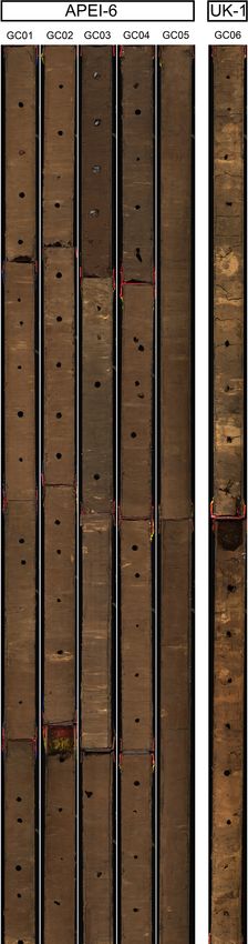
D.O.B. Jones et al. Progress in Oceanography 197 (2021) 102653
Thermoquest Scientific ISQ-LT mass spectrometer, see Jeffreys et al. 2.4. Faunal samples
(2009a). Concentrations of individual compounds were determined by
comparison of their peak areas with those of the internal standards and Macrofaunal samples were processed using live-sorting cold-chain
were corrected after calculation of their relative response factors (Kir protocol for DNA taxonomy (Glover et al., 2016a), which included at-sea
iakoulakis et al., 2004). abundance counts, morphological study and imaging. Sediments
(0–150 mm depth) were sieved at 300 μm and sorted cold under a dis
2.3.4. Environmental DNA and metabarcoding secting microscope. During collection, topwater was lost from several
Sediment was aseptically sampled from Megacores at the SW site. boxcores in the southwestern site (but not in the northeastern site) and
The following sediment depth layers were used for analysis of eDNA hence abundance data should be considered non-quantitative. Scaven
studies: 0–1, 1–2, 5–6, 10–12 and 22–24 cmbf. Genomic DNA was gers were sampled by means of a baited trap (Horton et al., 2020b)
extracted from sediment samples using the FastDNA Spin Kit for Soil deployed for < 40 h at two stations (JC120-008 and JC120-039; baited
(MP Biomedicals, USA) following the manufacturer’s protocol. Addi with tuna) at APEI-6 SW and a second trap type (Leitner et al., 2017) at
tional extraction blanks containing only the FastDNA Spin Kit reagents one station (AB02-TR13; baited with one mackerel) at APEI-6 NE.
were processed with the sediment samples. The concentrations of DNA Molecular methods and primers for markers 18S, 28S, 16S and
from all samples was below 0.1 ng mL− 1 and required further concen mitochondrial cytochrome oxidase subunit 1 (CO1) follow recom
tration. DNA was concentrated using Zymo Clean & Concentrator-5 kits mended protocols (Glover et al., 2016a). For this study, conspecificity
with a 2:1 DNA Binding Buffer ratio and eluted into 50 mL sterile, was confirmed at the molecular level using sequence alignment. Studies
DNase-free water. The V4 region of the 16S bacterial and archaeal rRNA in preparation, and already published, will include full phylogenetic
gene was amplified by the polymerase chain reaction (PCR) using the analyses of groups in question (e.g. Wiklund et al., 2017). Data for in
oligonucleotide primers Pro515f/Pro805r. These also contain Illumina dividual samples, identifications, materials, DNA vouchers and types are
adapter sequences and sample-specific barcode sequences (Caporaso reported in ongoing taxonomic publications (Dahlgren et al., 2016;
et al., 2012; Caporaso et al., 2011). The amplified 16S rRNA gene Glover et al., 2016b; Wiklund et al., 2017). We do not report here studies
products and extraction blanks were sequenced using an Illumina MiSeq of Crustacea, but include all other metazoan taxa, for which sequences
at the National Oceanography Centre, Southampton. Illumina paired- were available. Data from within the study areas (APEI-6 and UK1) from
end 16S rRNA reads were joined and analysed with QIIME (Quantita JC120, AB01 and AB02 were used to compare the APEI-6 region with the
tive Insights Into Microbial Ecology) microbiome analysis package, exploration contract sites.
version 2–2017.9 (Caporaso et al., 2010). The DADA2 pipeline within
QIIME 2 was implemented for sequence quality control and chimera 2.4.1. Autonomous seabed photography
removal. Operational Taxonomic Units (OTUs) that were observed in the Vertically-facing seabed photographs were collected in APEI-6 SW
PCR blanks were considered to be contaminants and were filtered from using the autonomous underwater vehicle (AUV) Autosub6000 (camera:
the samples. Taxonomy was assigned using the Silva 132 database Grasshopper2, lens focal length: 12 mm, frame resolution: 2448 × 2048
(Quast et al., 2012). Taxa or OTUs were defined at 99% 16S rRNA gene pixels; photograph interval 850 ms) travelling (speed 1.2 ms− 1) along
identity. zig-zag image transects with random start points. The image data were
post-processed as described in Simon-Lledo et al. (2019a). The full
resultant dataset was composed of data from 88,630 non-overlapping
Fig. 1. Map of APEI-6 showing shipboard multibeam bathymetry for southwestern area (right) and northeastern area (lower left). Seamount investigated indicated
by black box on right figure. Top left map shows position of APEI-6 relative to nodule exploration contract areas (labelled by contractor) and nearest APEIs. The
extent of the SW and NE areas are indicated as red rectangles.
4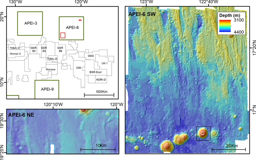
D.O.B. Jones et al. Progress in Oceanography 197 (2021) 102653
images collected at altitudes of 2–4 m, representing a seafloor area of SW. Thus, smaller sized animals could be potentially underestimated at
160,500 m2. A subset of 12 randomly-selected transects were used for the seamount, relative to the other locations. Because of the relatively
quantitative biological analysis (10,052 images, covering a seabed area small sample size at the seamount, only ecological measures that are less
of 18,582 m2). sensitive to small sample sizes were used (e.g. numerical density of
A total of 2571 images were obtained on one dive at APEI-6 NE using fauna (Simon-Lledó et al., 2019a)).
the AUV REMUS6000. The vehicle travelled at 1.5 ms− 1 while taking
photographs every 3.5 s at varying altitudes (5 cm] megafauna. elliptical field of view. The lander was baited with ~ 1 kg of Pacific
mackerel (Scomber japonicus), which was maintained in the centre of the
2.4.2. Towed-camera photography field of view 1 m in front of the cameras. Video was recorded in 2-minute
The UK National Oceanography Centre towed camera platform intervals with 8-minute rest periods to extend battery life to 24-hours
HyBIS was used to carry out video and photographic transects in more and to minimize light disturbance to bait-attending fauna.
topographically complex areas, such as the seamount investigated in
APEI-6 SW. HyBIS was equipped with two video camera systems 2.4.4. Automatic detection of nodules in images
(including parallel red lasers attached 110 mm apart for scaling). Video Nodule cover (%) was quantified from the AUV imagery collected at
was recorded using a forward-facing Bowtech L3C-550C video camera APEI-6 SW using the Compact-Morphology-based polymetallic Nodule
and a vertically-mounted Insite Pacific Super-Scorpio video camera. The Delineation method (CoMoNoD; (Schoening et al., 2017)). The CoMo
Super-Scorpio camera (lens focal length: 26.3 mm in air) was also used to NoD algorithm calculates the size of each nodule (i.e., seafloor exposed
take stills at 4 s intervals (frame resolution 4672 × 2628 pixels). A total area) detected in an image, enabling the calculation of descriptive
of 3106 frames were collected at the seamount. Each picture was clas nodule statistics. Note that it is currently not possible to relate directly
sified as imaging either exposed bedrock stratum (e.g. where pillow the image-based assessments of seabed nodule cover with those made by
lavas were visible), or sediment. direct sampling methods (Gazis et al., 2018; Schoening et al., 2017).
For subsequent quantitative analysis, frames taken too high (no red Only visible nodules ranging from 0.5 to 60 cm2 (i.e. with maximum
laser dots visible) or too low (taken before and after seafloor collisions) diameters of ~1 to ~10 cm) were considered for analysis to avoid in
above the seafloor were removed. Overlap between pictures was also clusion of large non-nodule formations. Average nodule densities were
manually removed by visualisation of consecutive remaining pictures. calculated on an image basis, whereas average nodule sizes were
This left 350 pictures for quantitative analysis, covering a total area of calculated on an individual nodule basis.
5,191 m2. On average, these were collected at a higher altitude above
seabed (mean altitude = 4.3 m, mode = 6.20 m) than at the other sites
imaged by AUV (mean altitude = 3.10 m, mode = 2.91 m) within APEI-6
Table 2
Summary of sample numbers used for analysis at APEI-6 and at UK-1 (on cruise JC120 only). Note some additional samples are available (See supplement S1). NA =
Not Available.
Parameter Method Sample Unit APEI-6 NE APEI- 6 SW APEI-6 SW UK-1 Notes
Samples Samples (not Seamount Samples
seamount) Samples (JC120)
Water temperature, Water sampling Regular (24 Hz) 1 6 1 1 Previously unpublished
salinity and oxygen rosette and sensor-based
sensors measurements
Nodule density, Box core One core (0.25 m2) 2 18 NA 1 Previously unpublished
dimensions and
weight
Seabed nodule Photography Photographs (~1.7 0 197,900 NA 0 See Simon-Lledo et al., 2019b
coverage (automated m2)
processing)
Grain size, sediment Megacore One core (0.0079 0 19 1 1 See Simon-Lledo et al., 2019a for grain
biogeochemistry m2) size; Biogeochemistry results
previously unpublished
Sediment metals Megacore One core (0.0079 0 4 0 1 See Menendez et al., 2019
m2)
Sediment oxygen Gravity core One core 0 5 0 1 Previously unpublished
penetration
Macrofaunal species Box core Total of all box cores NA 15 NA 1 Previously unpublished
richness
Benthic megafauna Photography Photographic NA 12 NA 0 See Simon-Lledo et al., 2019a
and trace properties (manual transect (1320 m2)
annotation)
Qualitative megafauna Photography Total area (m2) 21853.5 NA 5191 NA Previously unpublished
and habitat (manual
description assessment)
Microbes Megacore Subsamples from NA 96 NA 6 JC120 results previously unpublished.
one core Additional material from APEI-6 NE in
Wear et al. (2021) and Lindh et al.
(2017)
5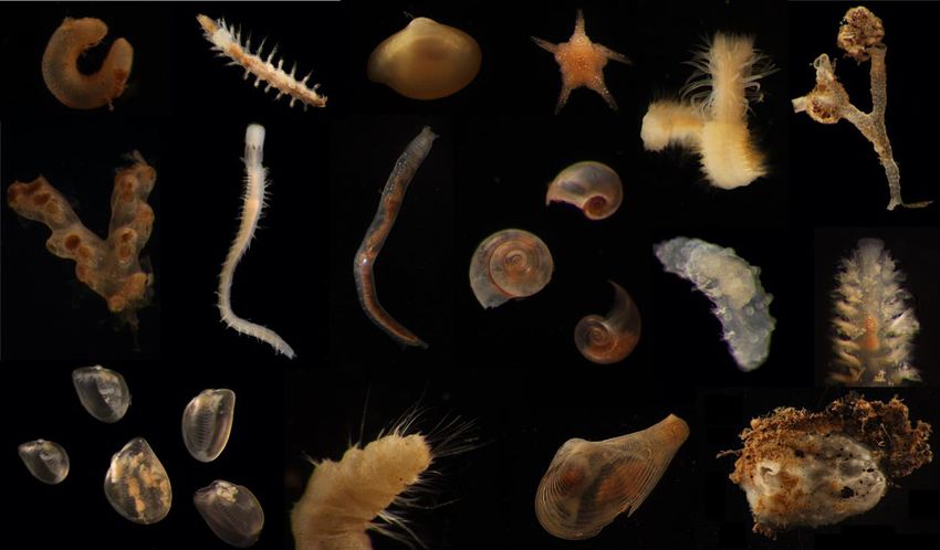
D.O.B. Jones et al. Progress in Oceanography 197 (2021) 102653
2.5. Detection and classification of megafauna in images LCPW is the coldest (Θ < 1.2 ◦ C) densest water mass with high salinity
and high oxygen levels owing to its relatively recent ventilation. In
Megafauna specimens (>10 mm) in selected quantitative imagery contrast, NPDW is the oldest low-oxygen water mass formed internally
were identified up to the lowest taxonomic level possible and measured without surface sources from the upwelled LCPW in the North Pacific
using either BIIGLE software (Bielefeld Image Graphical Labeller and (Kawabe and Fujio, 2010). In the CCZ, this water mass is somewhat
Explorer; (Langenkämper et al., 2017)) for the APEI-6 SW images, or warmer (1.2 < Θ < 2 ◦ C) than the LCPW and flows southward in the
Image J (Schneider et al., 2012) for the APEI-6 NE dataset. Several re eastern CCZ, along the western flank of the East Pacific Rise, which is to
visions were performed to ensure consistency of fauna morphotype the east of APEI-6.
identifications with a megafauna catalogue developed upon interna Breaks in the slopes of the SA/Θ and O2/Θ curves between APEI-6 SW
tional taxonomic expert consultations (Simon-Lledó et al., 2020), and the UK1 study area (Fig. 2: a and b) indicate differences in the deep-
providing a standardised megafauna morphotype (mtp) code. Mega water mass separation, which occurs on a colder isotherm at APEI-6 (Θ
fauna are assigned a standardised open nomenclature (Horton et al., = 1.23 ◦ C) than at UK1 (Θ = 1.30 ◦ C). This observation is consistent with
2021). Quantitative seabed megafauna data collected at the UK1 AB01 an expected decrease in the volume of northward flowing LCPW be
area (Amon et al., 2016) was reassessed and aligned in accordance with tween UK1 and APEI-6. It is not known if the changes in water masses
this standardized catalogue to enable direct comparisons between observed are sufficient to lead to other environmental effects, as they are
different areas. In addition, large (>5 cm) megafauna visible in images elsewhere (Puerta et al., 2020; Reinthaler et al., 2013).
collected at the APEI-6 NE area were also identified but not quantified. Current speed data are very limited in APEI-6. A single 24-hour
Invertebrates living in a shell or tube (e.g. most polychaete and deployment (Leitner et al., 2017) at APEI-6 NE recorded very low
gastropod taxa) were excluded from analyses. Paleo-geological features average (0.03 m s− 1) and maximum (0.23 m s− 1) bottom current speeds.
observed on the seafloor were annotated and measured, including: Currents of the bottom 50–100 m in the CCZ are typically below 0.05 m
whale bones and shark teeth, Paleodictyon nodosum facies, and any s− 1 when averaged over several months (Hayes, 1979). However,
non-polymetallic nodule (angular shaped) geologic formations, from mesoscale features affect deep velocities and events with amplitudes >
cobbles to large rocks. Identifications were improved by referencing to 0.1 m s− 1 can last several weeks (Kontar et al., 1994). Peak velocities of
collected specimens. up to 0.25 m s− 1 have been registered (Aleynik et al., 2017; Amos and
Roels, 1977). Deep low-frequency currents intensify in the bottom
3. Results and discussion boundary layer within ~ 100–30 m from the seabed in this region and
veer counter-clockwise toward the bottom consistent with an Ekman
3.1. Oceanography layer dynamic (Hayes, 1980; Kontar and Sokov, 1994). In addition,
higher-frequency internal inertia-gravity waves, including semidiurnal
The deepest water masses of the CCZ consist of Lower Circumpolar tides and near-inertial waves, are generated by barotropic tides, eddies
Water (LCPW) and North Pacific Deep Water (NPDW) (Johnson and and mean currents flowing over rough topography, which includes
Toole, 1993). CTD profiles at APEI-6 indicate the presence of low- seamounts, ridges, and troughs present in the APEI-6 area. These in
salinity (34.86 SA) and low-oxygen (2.65 mL L-1) NPDW around 3600 ternal waves and the associated turbulence may act to amplify the
m (Θ > 1.30 ◦ C), but also the eastward penetration of saline and more dispersion of potential mining-related plumes (Aleynik et al., 2017).
oxygen-rich LCPW below the NPDW layer extending as far as UK1
(117◦ W). The presence of LCPW this far east in the tropical Pacific is
unexpected. LCPW enters the CCZ from the west, south of the Hawaiian 3.2. Seabed morphology
Ridge around 160◦ W, before travelling north-northeastwards (Juan
et al., 2018). LCPW is formed of North Atlantic Deep Water (NADW) and The area surveyed for this study covers approx. 6,300 km2 in APEI-6
Antarctic Bottom Water (AABW), which originate from the North SW and 380 km2 APEI-6 NE, representing around 4.1% of APEI-6
Atlantic and the Weddell Sea, respectively (Wijffels et al., 1996). The (Fig. 1). Water depths at APEI-6 SW range from 3400 m on the tallest
seamount down to 4400 m in the deepest parts surveyed. APEI-6 SW
Fig. 2. (a) Absolute Salinity SA and (b) dissolved oxygen concentration versus Conservative Temperature Θ for the CTD profiles taken in APEI-6 SW and UK1 regions.
Note that Conservative Temperature and Absolute Salinity are not the same as in situ temperature and practical salinity, as measured by the CTD.
6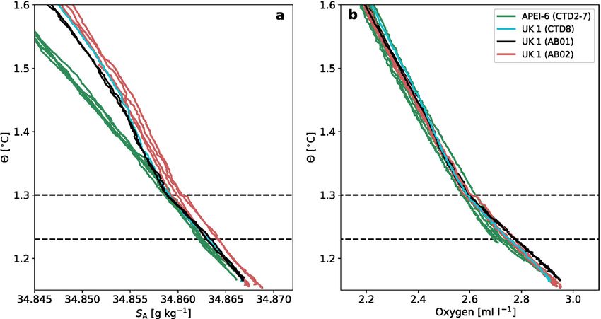
D.O.B. Jones et al. Progress in Oceanography 197 (2021) 102653
contains an E-W orientated chain of seamounts/knolls (see seamount et al., 2011; Winterer and Sandwell, 1987). The rugose topography of
section for more detail) in the southern half, and a sequence of ridges, the CCZ is caused by tectonic processes connected to the formation of the
flatter areas and troughs (horst-and-graben structure) in the northern East Pacific Rise, which lies to the east (Wessel et al., 2006) and low
half of the study area, with a few seamounts/knolls scattered in between sedimentation rates have limited homogenisation of the topography by
these two areas. The horst-and-graben morphology has a NNW-SSE sediment blanketing (Juan et al., 2018). At APEI-6, sub-bottom profiles
orientation and covers depths between 3850 m and 4350 m. Troughs indicate up to three acoustic units of sediment, with the uppermost
are on average spaced ca. 15 km apart. This morphology appears char (AU3) likely comprised of unconsolidated sediments up to 18 m thick, a
acteristic of the remainder of APEI-6 (Washburn et al., 2021) and the deeper distinct layer (AU2) of older (possibly Miocene) consolidated
CCZ in general (Haxby and Weissel, 1986; Juan et al., 2018; Rühlemann sediments and in some places a third high-amplitude unit (AU1), likely
Table 3
Average and 95% confidence intervals for parameters measured across APEI-6 and other relevant areas. Contract areas: German Federal Institute for Geosciences and
Natural Resources (BGR) eastern contract area; UK1: UK Seabed Resources Limited eastern contract area; L’Institut Français de Recherche pour l’Exploitation de la Mer
(IFREMER); InterOcean Metals contract area (IOM). For nodule dimensions n: number of nodules measured, l = length, w = width, h = height.
Parameter APEI-6 SW APEI-6 NE APEI-6 Seamount Contract areas Reference for contract area values
Average depth, m 4200 4000 3500 4110: UK1 This study
4840: BGR W1 Rühlemann et al. 2011
4240: BGR E1
Area size, km2 6,300 380 36 60,000: UK1 Rühlemann et al. 2011
17,000: BGR W1
58,000: BGR E1
Seabed Temperature (in situ), ◦ C 1.54 1.55 1.51: UK1 this study
Seabed Conservative Temperature, Θ 1.20 1.29 1.17: UK1 this study
Seabed salinity (practical salinity) 34.68 34.68 34.69: UK1 this study
Seabed Absolute Salinity (SA, g kg− 1) 34.86 34.86 34.87: UK1 this study
Seabed Oxygen, mL L-1 2.80 2.61 2.91: UK1 this study
Nodule density, no m− 2 314 (212–423) 16: UK1 this study
Nodule dimensions, mm n = 1417 nodules; n = 1260 : UK1 Smith et al. 2013; Rühlemann et al. 2011;
l = 19.8 (19.4–20.3) l = 39 ± 8 : UK1 Veillette et al., 2007a,b
w = 15.5 (15.1–15.8)
h = 9.2 (9.0–9.4) l = 40–80: BGR E1
l = 40–75: IFREMER E
2
Nodule weight, kg m− 1.33 (0.81–1.9) 1.7: UK1 (1 box core) this study
1.7–57: UK1; Rühlemann et al. 2011
8.0: BGR W1;
13.7: BGR E1
Seabed nodule coverage (%) 6.6 (SD 4.9)
range = 0–48
Grain size, µm (sample means, min - 0 to 5 cm: 6.53–9.21 0 to 5 cm: 27.62 UK1: this study
max) 5 to 10 cm: 5 to 10 cm: 21.72 0 to 5 cm: 18.06
6.19–11.16 10 to 15 cm: 15.97 5 to 10 cm: 17.6
10 to 15 cm: 15 to 20 cm: 17.43 10 to 15 cm: 17.58
5.72–20.08 15 to 20 cm: 18.74
15 to 20 cm:
5.68–20.15
Total Organic Carbon (TOC, %) 0.43 ± 0.03 0.22 0.71: UK1 this study
0.62: BGR Volz et al., 2018
0.52: GSR
0.24: APEI-3
Total Nitrogen (TN, %) 0.01 ± 0.004 0.06 0.14: UK1 this study
molar TOC:TN ratio 4.62 ± 0.14 4.50 5.7: UK1 this study
CaCO3, % 0.4 ± 0.09 73.3 0.1: UK1 this study
Sediment oxygen penetration depth, m >2 1: UK1 this study Volz et al., 2018
1: GSR
3: IOM
Fe (wt %) 6.75 ± 1.29 6.06 ± 0.105: UK1 this study
Mn (wt %) 27.4 ± 2.12 28.2 ± 3.01: UK1 this study
Mn:Fe 4.06 4.65: UK1 this study
Cu (ppm) 9770 ± 2150 7980 ± 640: UK1 this study
Ni (ppm) 12700 ± 1630 10600 ± 1130: UK1 this study
Co (ppm) 2500 ± 666 1220 ± 90.1: UK1 this study
ΔREY (ppm) 1000 ± 340 813 ± 38.4: UK1 this study
Al (wt %) 2.31 ± 0.238 2.04 ± 0.165: UK1 this study
P (wt %) 0.12 ± 0.01 0.13 ± 0.01: UK1 this study
Li (ppm) 103 ± 25.2 173 ± 4.32: UK1 this study
Macrofaunal species richness 25 this study
Megafaunal xenophyophore density, 2.55 (1.74–3.32) NA 0.19 0.65 (0.51 – 0.78): UK1 Amon et al 2016
ind. m− 2
2
Megafaunal metazoan density, ind. m− 0.38 (0.28 – 0.46) NA 0.07 1.08 (0.76–1.25): UK1 Amon et al. 2016; Simon-Lledó et al. 2020
0.44: TOML-D
2 2
Megafaunal metazoan taxon richness, 123 (in 18,852 m of 34 (in 850 37 (in 5120 m of 110 (in 4204 m2 of seabed): Amon et al. 2016; Simon-Lledó et al. 2020
total morphospecies seabed) m2) seabed) UK1
189 (in 20200 m2 of
seabed): TOML-D
2
Paleodictyon density, trace m− 0.33 0 Durden et al. 2017
7
D.O.B. Jones et al. Progress in Oceanography 197 (2021) 102653
bedrock, which outcrops in places (Alevizos et al., submitted). available nodule size distribution data are limited.
Nodule density (mean 200 – 632 m− 2), size (maximum dimension
16.1 – 21.9 mm), and estimated resource by mass (0.55–2.56 kg m− 2)
3.3. Nodules
varied at the landscape scale across APEI-6 SW (Table S2). Average
nodule coverage calculated from seabed photographs at the APEI-6 SW
The shape (sub-spherical with smooth surfaces) and size (mean
was 6.6 % (Table 3), again with high spatial variation (Table S2; Fig. 3:
maximum diameter ~ 20 mm) of nodules recovered across APEI-6 SW
c-d). These variations are consistent with local variations observed
were smoother and smaller than those measured at UK1 (mean
across morphologically different seafloor areas within the BGR license
maximum diameter 39 mm from ABYSSLINE surveys), IFREMER (Veil
area in the eastern CCZ (Mewes et al., 2014; Peukert et al., 2018; Rüh
lette et al., 2007b), E1 BGR (Rühlemann et al., 2010) and the eastern
lemann et al., 2011), where nodule resource (0.2–30 kg m− 2) and size
CCZ (IOM, (International Seabed Authority, 2010); Table 1). Caution
(10–120 mm) varied at a similar spatial scale of tens to hundreds of
should be taken in making direct comparisons as nodule size distribu
metres. Regional scale investigations suggest nodule abundances are
tions are variable even across fine scales (tens of metres) and publicly-
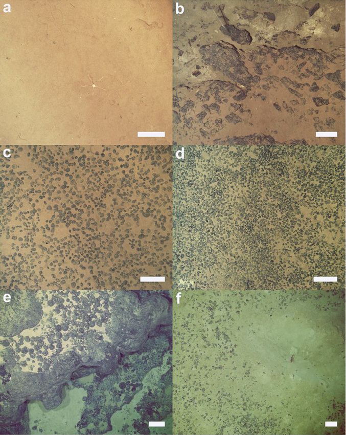
Fig. 3. Representative images of seafloor in different areas of APEI-6-SW. a to d: collected using Autosub6000. e to f: collected using HyBIS towed camera. a) Nodule-
free seabed. b) Exposed bedrock, boulders, and cobble seabed. c) Densely nodule-covered seabed (35% coverage). d) Densely nodule-covered seabed (47% coverage).
e) Fe-Mn crust coated pillow basalt and cobble seabed at the western flank of the seamount crater. f) Fine sediment and talus fragments seabed at the centre of the
seamount crater. Scale-bars represent 25 cm.
8
D.O.B. Jones et al. Progress in Oceanography 197 (2021) 102653
higher in the central CCZ than at the periphery, where most of the APEIs
are located (McQuaid et al., 2020). In general, the mass per unit area of
the nodules is controlled more by the size of the nodules rather than
their numerical density (Rühlemann et al., 2011). This variation in
nodules is typically attributed to variations in sedimentation, including
those related to topography (Juan et al., 2018; Mewes et al., 2014;
Rühlemann et al., 2011).
3.3.1. Nodule composition
The nodules consist of alternating concentric layers of Mn-rich ox
ides (birnessite) and Mn-Fe-rich oxyhydroxides (vernadite); small
quantities of aluminosilicate-rich detrital material and minor quantities
of fluorapatite occur in pore spaces (expanded in Menendez et al 2019).
Phillipsite, a marker of volcanic activity, was present in the nodules
assessed from APEI-6 SW but not UK-1 (expanded in Reykhard and
Shulga, 2019). Compared to nodules from the UK1 contract area, and
other parts of the CCZ, APEI-6 SW nodules have on average slightly
higher concentrations of Fe (6.75 wt%), Co (2500 ppm) and total rare-
earth elements (1000 ppm), and lower concentrations of Mn (27.4 wt
%) and Li (103 ppm) (Table 1). There is little variation in the chemical
composition of nodules within APEI-6 (expanded in Menendez et al.,
2019). Together with the small size of the nodules, their chemical
composition indicates that the APEI-6 nodules acquire a greater part of
their metals from a hydrogenous source (seawater) relative to a diage
netic source (sediment pore waters) compared to other parts of the CCZ
assessed to date (Bau et al., 2014; Hein et al., 2013; Menendez et al.,
2019; Reykhard and Shulga, 2019).
3.4. Sediment properties
The visual appearance of the seafloor (Fig. 3) showed soft sediments,
nodules and regular features associated with bioturbation (mounds,
trails and faecal deposits). Larger pits in the sediment of probable
biogenic origin (expanded in Marsh et al., 2018) were seen in side-scan
sonar data. These are hypothesised to result from the feeding activities
of beaked whales and also occur in UK1 (Marsh et al., 2018), on
seamount summits in APEI-4 and 7 (Leitner et al., submitted) as well as
other areas in the Pacific (Purser et al., 2019). Occasional rock outcrops
were observed (Fig. 3: b,e; (Alevizos et al., submitted)).
Radiolarian-bearing pelagic sediments were common across APEI-6
SW. These fine-grained muds are consistent with other seabed sedi
ments across the wider CCZ (Mewes et al., 2014). Surface sediments
(0–5 cm) at APEI-6 SW were dominated by clay to fine silt particles <
7.8 μm (58–68 % of dry weight), and medium to very coarse silt grains
7.8–63 μm (28–39 %). As found elsewhere, clays at APEI-6 SW were in
most cases poorly crystallized smectite, sometimes also illite and quartz;
feldspar and chlorite occur less frequently (Riech and von Grafenstein,
1987). Deeper sediments (5–20 cm) at the deep plain and flat followed
this same pattern, whereas replicate cores at the ridge and trough sites
were more heterogeneous, with median values ranging from 5.9 to 31.8
μm (see Table S4). Similar granulometries (~70% particles < 6.3 µm)
were found on surface sediments at the E1 BGR contract area (Mewes
et al., 2014), slightly finer grain sizes (median: 2–4 μm) were reported Fig. 4. Photographs of sectioned gravity cores from APEI-6 (GC01-05) and
within APEI-4 (western CCZ) and within the SE IFREMER contract area UK1. The image is cropped to the length of the shortest core (GC06). For scale,
(Halbach et al., 1979; Renaud-Mornant and Gourbault, 1990), whereas the width of each core is 70 mm.
within the UK1 contract area the median grain size was much coarser,
and described a bimodal size distribution pattern increasing with depth obtained at UK1 (on JC120). Buried nodules have been found more
(see Table S4). commonly in other samples elsewhere in the CCZ (Mewes et al., 2014)
In APEI-6 SW the gravity cores (Fig. 4) consisted of a fine mud, including from other samples at UK1 (Smith et al., 2013). Usually,
consistently of reddish brown colour with no notable layers although sediments in the CCZ have 2–3 lithostratigraphic units of variable
there were occasional white inclusions at various depths within the thickness comprising sediments from Late Eocene to Quaternary age
cores. Nodules were usually only found on the surface of the cores. On (Riech and von Grafenstein, 1987) and mainly consist of radiolarian and
very few occasions were nodules found deeper (e.g. at 17 cm depth in a diatom-bearing silty clay (Mewes et al., 2014). No information on
gravity core (JC120-GC2) at the trough site; Fig. 4) but no Mn-nodules or sedimentation rates at APEI-6 is available.
Mn-nodule fractions were found in the deeper parts of the sediments. The porosity of the sediment was similar in the different APEI-6
These characteristics were also shared with the single gravity core
9D.O.B. Jones et al. Progress in Oceanography 197 (2021) 102653
cores, with only little downward compaction (decreasing from ~ 0.9 ϕ SW (Table S5). A wide variety of compounds were identified at APEI-6
[ratio of volume of void space to total volume of material] close to the SW (111 in total) from both marine and terrestrial sources. However,
sediment surface to ~ 0.8 ϕ at 3 m). In the UK1 contract area the sedimentary organic material was predominantly marine in origin, as
porosity was slightly higher at the sediment surface (~0.95 ϕ) and indicated by TOC:TN ratios, (see above) and lipid biomarkers, e.g., the
changed even less with depth (~0.85 ϕ at 2 m). The UK1 information is C16/C26 fatty acid ratio, an indicator of the relative contribution of
only based on one core, which may not be representative of the whole marine (C16) vs. terrestrial (C26) organic matter (Meyers et al., 1984),
site. which ranged from 2 to 20 (mean = 6.3 ± 4.6 S.D.).
3.5. Sediment geochemistry 3.6.3. Sources and quality of organic matter
Phytodetritus is an important food source for deep-sea organisms at
Porewater nitrate concentrations were around 50 μmol L-1 and APEI-6 SW. Components of this material include dietary fatty acids that
stayed constant throughout the core in both APEI-6 SW and UK1. The are required for reproduction, growth, cell membrane structure and
nitrate profiles are similar to other CCZ studies (Jeong et al., 1994; function, energy storage and hormone regulation (Neto et al., 2006).
Mewes et al., 2014) and suggest that organic matter degradation is Lipid profiles at APEI-6 SW showed characteristics of phytodetrital
largely driven by oxic respiration. Low levels of organic carbon degra input, including short chain saturated fatty acids (D.O.B. Jones et al. Progress in Oceanography 197 (2021) 102653
(ACL = 29), with the C31 homologue being the next most prevalent some groups were more abundant in deeper sediment fractions at both
alkane. The carbon preference index (CPI) of n-alkanes averaged ~ 7.5; sites, such as Cyanobacteria and Betaproteobacteria in the 10–12 cmbf
this, combined with an ACL of C29, is a clear indication of a contribution and 20–22 cmbf layers. Cyanobacterial OTUs occurred in very low
of higher plant waxes to the sediments (Brassell and Eglinton, 1983). relative abundance in the top 0–6 cmbf of sediment at all sites. These
Similarly, high molecular weight (HMW) fatty acids yielded a mean CPI cyanobacteria comprised the ML635J-21 lineage within the Melaina
of ~ 6, suggesting the source of HMW fatty acids is from higher-plant bacteria class, a group of non-photosynthetic cyanobacteria (Soo et al.,
derived organic matter (Gagosian and Peltzer, 1986; Kawamura et al., 2014).
2003; Ohkouchi et al., 1997). This has been previously documented for
sediments in the Pacific despite the distance from land, with the domi 3.7.2. Macrofauna
nant mechanism of transport for this soil- and plant-derived terrestrial The macrofauna (some common representatives are shown in Fig. 5)
organic matter ascribed to aerosols (Gagosian and Peltzer, 1986; was dominated by annelids and isopod crustaceans noted elsewhere in
Kawamura et al., 2003; Ohkouchi et al., 1997). the CCZ (Glover et al., 2002; Hessler and Jumars, 1974; Janssen et al.,
A high abundance of C27, C29, C31 n-alkanes of terrestrial origin was 2019; Paterson et al., 1998). Although the foraminifera are typically
also observed in the APEI-6 SW and UK-1 nodules collected by trawl on abundant in the CCZ (Gooday et al., 2015; Mullineaux, 1987; Veillette
JC120 (expanded in Shulga, 2018). The CPI ~ 3 in nodules indicates the et al., 2007a), these have not been studied systematically in APEI-6
presence of more biodegraded organic matter compared to underlying samples. Data are therefore limited to the metazoan component. Mac
sediments. High concentrations of C16, C18, C20 n-alkanes and iso-, rofaunal abundance was dominated by crustaceans, sponges, annelids,
anteiso- C16 fatty acids associated with microbial degradation of organic cnidarians, molluscs, and others (including Brachiopoda, Chaetognatha,
matter confirm the occurrence of active bacterial processes within the Chordata, Nematoda, Platyhelminthes and unidentified taxa). The most
nodules (Shulga, 2018). These differences in biogeochemistry may help common macrofaunal species in APEI-6 SW was the sponge Plenaster
explain the differences in bacterial community structure between the craigi Lim & Wiklund, 2017 (expanded in Taboada et al., 2018), a
nodules and sediments observed in APEI-6 NE, OMS and UK-1 samples demosponge originally described from the OMS contract area, adjacent
(Lindh et al., 2017). to UK-1 (Lim et al., 2017). Mean densities of 12 ± 6.2 individuals m− 2
observed for the sponge across APEI-6 SW, corroborates the suggestion
3.7. Biological composition that P. craigi might be the most common sessile metazoan occurring in
the CCZ (Lim et al. 2017). In APEI-6 SW, P. craigi density was positively
3.7.1. Bacteria and Archaea correlated to the number of nodules. We detected molecular affinities
Branched fatty acids, generally indicative of anaerobic bacteria, between samples of P. craigi from APEI-6 SW and UK1 Stratum A, despite
accounted for 1–14% of the total surface sediment lipid pool at APEI-6 a separation of ~ 800 km. Migration analysis in Taboada et al. (2018)
SW (Gillan and Johns, 1986). Hopanoids, mainly indicative of aerobic inferred very little progeny dispersal of individuals between areas and
bacteria, accounted for 3–16% of the total lipid pool at APEI-6 SW hydrodynamic models suggested a prevalent northeasterly transport
(Ourisson and Rohmer, 1992). Arachidonic acid, C20:4(n-6) was the trajectory, i.e., from exploration contract areas to APEI-6 SW.
dominant PUFA in the sediments at APEI-6 SW, constituting ~ 40% of A total of 16 macrofaunal (infauna and encrusting fauna) taxa from
the PUFA pool. This fatty acid has been linked to piezophilic bacteria six phyla (Annelida, Bryozoa, Echinodermata, Mollusca, Porifera and
(Fang et al., 2004; Fang et al., 2006) and is present in high concentra Sipuncula; note that the Arthropoda were present but not processed)
tions in some echinoderms (Drazen et al., 2008; Howell et al., 2003; were confirmed with both morphological and molecular data to occur in
Jeffreys et al., 2009b; Mansour et al., 2005). both APEI-6 boxcores and UK1 exploration contract areas (Table S6).
Environmental metabarcoding (described in the rest of the section) These data indicate species ranges of ~ 500 km (i.e. across APEI-6 SW
of 30 sediment samples from the APEI-6 SW area yielded a total of and NE sites) and between APEI-6 and UK1 exploration areas separated
12,836 bacterial and archaeal OTUs (operational taxonomic units; by ~ 1000 km. An additional 24 taxa were only detected in APEI-6 NE.
sharing 99% sequence identity) from 153,000 16S rRNA gene sequences Investigation of the population-level connectivity of the widespread
(expanded in Hollingsworth et al., 2021). Of these OTUs, 20.23% were species based on sequences from additional individuals is ongoing
classified as Archaea, 79.34% as Bacteria and 0.43% could not be (Dahlgren et al. in prep.).
assigned to domain level (Unassigned). These data allow the first test of the hypothesis of Glover et al (2002)
Across all studied abyssal plain sites of the APEI-6 SW and UK1 that there is a core group of abundant, widespread species that can range
contract area, sediment microbial assemblages were dominated by
members of the Thaumarchaeota, Alphaproteobacteria, Gammaproteo
bacteria and Planctomycetes. The Nitrosopumilus genus in the archaeal
Thaumarchaeota group were enriched in the sediments. Members of the
Thaumarchaeota group are chemolithoautotrophic nitrifiers, capable of
oxidising ammonia (Könneke et al., 2005). The genus Nitrospira (2%
relative abundance of sequences) is capable of nitrite oxidisation (Koch
et al., 2015) and has been previously reported in similar proportions in
CCZ sediments (Shulse et al., 2017)
As a group, the Proteobacteria represented the largest proportion of
the sediment microbial assemblages at APEI-6 SW and UK1, followed by
the Thaumarchaeota. Both showed variation between sites at APEI-6 SW
and UK1. Thaumarchaeota formed a higher proportion of the commu
nity in the deeper sediment layers (20–22 cmbf) at APEI-6, whilst at
UK1, this group was more abundant in the top two centimetres in the
JC120 data. Other major groups also displayed spatial variation through
Fig. 5. Microscope images of macrofauna. Upper row from left to right: Apla
the sediment. Actinobacteria, Bacteroidetes, Deltaproteobacteria, cophora indet, Anguillosyllis sp., Ledella sp., Echinodermata juvenile indet.,
Gammaproteobacteria and Nitrospirae were more enriched in the 0–6 Aglaophamus sp., Bryozoa indet. Middle row from left to right: Bryozoa indet.,
cmbf fraction of sediments at both the APEI-6 SW and UK1 sites. Glycera sp., Ophelina martinezarbizui Wiklund et al., 2019, Gastropoda indet.,
Chloroflexi were also more abundant in surface sediments across APEI-6 Sphaerodoridae indet., Laonice sp. Lower row from left to right: Dacrydium sp.,
SW, but not at UK1, where the reverse pattern was observed. Conversely, Flabelligeridae indet., Myonera sp., Plenaster craigi Lim & Wiklund, 2017.
11D.O.B. Jones et al. Progress in Oceanography 197 (2021) 102653
freely across the eastern tropical Pacific abyssal plain at scales of at least Gray 1828 sp. inc. (formerly Plesiopenaeus armatus (Spence Bate 1881))
1000 km. This hypothesis is now supported by some molecular evidence. and Hymenopenaeus nereus (Faxon 1893) sp. inc., and the brittle star
However, it is not yet possible to ascertain degrees of endemism, if any, at Ophiosphalma cf. glabrum (Lütken & Mortensen, 1899) (formerly
particular sites, as all sites (in particular the APEI-6) are under sampled. Ophiomusium glabrum Lütken & Mortensen 1899). These taxa were all
The presence of 24 taxa only detected in APEI-6 is suggestive of some common in the UK1 license areas but the total scavenger species richness
degree of turnover (Paterson et al., 1998) but given the level of under in APEI-6 NE was much lower than in those other areas. Regional
sampling, they cannot be described as ‘endemic’ to the APEI-6 region. In variation in the scavenging community is apparent from across the CCZ
addition, studies (Stewart et al in prep) of an additional ~ 3000 specimens (Drazen et al., 2021). However, in this case, a single deployment was
from the UK1 and OMS regions reveal many taxa that are not found in inadequate to fully characterize the fauna in APEI-6 (Leitner et al.,
APEI-6, with probably many absences owing to under sampling of APEI-6. 2017).
The general pattern is in agreement with a molecular-only study of the
BGR and IFREMER exploration areas (Janssen et al., 2015), in which 95 3.8. Megafauna
out of 233 polychaete molecular operational taxonomic units (MOTUs)
were shared across distances of 1300 km, but perhaps differs from their 3.8.1. Metazoa
finding that just two out of 95 isopod MOTUs were shared across that Megafauna (metazoans > 1 cm) across APEI-6 SW (Fig. 6) were
distance. Common polychaetes and isopods showed molecular connec dominated by soft corals and anemones (Order Alcyonacea: 32.8% of
tivity among populations between the IFREMER and BGR exploration total abundance; Order Actiniaria: 11.7 %), sponges (Class Demo
areas of all species investigated (Janssen et al., 2019), although they spongiae: 10.1%; Class Hexactinellida: 1.3%; Porifera indet.: 7.1%),
inferred weak barriers to gene flow for the isopod species, probably related echinoderms (14.6 %), bryozoans (11.3%), and arthropods (Subphylum
to the fact that the species under study are brooders and hence have Crustacea: 7.4%). Fishes, tunicates, annelid worms and ctenophores
limited dispersal abilities. In a recent study of harpacticoid copepod spe were also found in much lower proportions ( 5 cm minimum dimension at APEI-6 NE, rather
12D.O.B. Jones et al. Progress in Oceanography 197 (2021) 102653
Fig. 6. Examples of seafloor metazoan megafauna photographed at the abyssal plain sites of APEI-6 SW during AUV survey. Scale bars representing 5 cm. CCZ-
standardised megafauna morphotype (mtp) codes in capital letters. a to f: Abundant taxa (density = 50–400 ind. ha− 1) . g to l: Scarce taxa (density < 5 ind.
ha− 1). a) Demospongiae indet. mtp-POR_002, higher density in areas with low nodule abundance. b) Actiniaria stet. mtp-ACT_022 and c) Farciminariidae indet. mtp-
BRY_005, higher density in areas with mid nodule abundance. d) Lepidisis gen. inc. mtp-ALC_005, higher density in areas with mid to high nodule abundance. e)
Munnopsididae indet. mtp-ART_001 and f) Spatangoida indet. mtp-URC_012. g) Hymenaster pellucidus sp. inc. (AST_012) h) Cerataspis monstrosus Gray, 1828 sp. inc.
(DEC_001). i) Benthodytes indet. mtp-HOL_037. j) Actiniaria stet. mtp-ACT_010. k) Metridioidea stet. mtp-ACT_042. l) Saccocalyx pedunculatus sp. inc. (HEX_020).
than the > 1 cm minimum dimension used in the analysis of APEI-6 SW) and 15 times higher respectively at UK1 than at APEI-6. While further
and six fish taxa, all of which were shared with the SW except for two regional synthesis work is needed to better understand biogeographical
holothurian morphotypes. Note that the APEI-6 NE images were not as variations across the CCZ and within the APEI-6 and UK-1 areas, pre
high quality or analysed in as much detail as the APEI-6 SW images and liminary comparisons of the APEI-6 megafauna with other areas (e.g.
no quantification was made of faunal densities. Almost half (48%) of the Simon-Lledó et al., 2020; this study) suggest a low similarity (and thus
invertebrate morphotypes (>1 cm) found in APEI-6 (NE and SW sites potentially low representativity) of the megabenthic assemblages of this
combined) were also encountered at the UK1 area (reassessed from protected area compared to areas studied in UK1 and TOML contract
Amon et al 2016) where a total of 110 morphotypes were identified from areas.
the 4470 invertebrate specimens detected in quantitative image surveys.
The assemblages of these two areas also substantially differed in the 3.8.2. Protista
relative abundance of several of the dominant taxonomic groups. For Xenophyophores (giant foraminifera) are exceptionally diverse in
instance, sponges and soft corals were respectively 2 and 4 times more the CCZ (Gooday et al., 2020a; Gooday et al., 2017b). Nine species were
abundant in UK1, while the density of anemones was 3 times higher in recognised in samples collected in APEI-6 NE during AB02. In seafloor
APEI-6 study areas. Most remarkably, among the mobile fauna, echinoid photographs from APEI-6 SW, the mean density of xenophyophores was
(sea urchins) abundance was almost twice as high in APEI-6 than at UK1. 2.59 ind. m− 2 (CI95 ± 0.79) but values varied across the region
Densities of asteroids (sea stars) and ophiuroids (brittle stars) were 35 (Table S3), with maximum recorded densities per image reaching 17
13You can also read