Prime factorization using quantum variational imaginary time evolution
←
→
Page content transcription
If your browser does not render page correctly, please read the page content below
www.nature.com/scientificreports
OPEN Prime factorization using quantum
variational imaginary time
evolution
Raja Selvarajan1, Vivek Dixit1, Xingshan Cui2,3, Travis S. Humble3 & Sabre Kais1,3*
The road to computing on quantum devices has been accelerated by the promises that come from
using Shor’s algorithm to reduce the complexity of prime factorization. However, this promise hast
not yet been realized due to noisy qubits and lack of robust error correction schemes. Here we explore
a promising, alternative method for prime factorization that uses well-established techniques from
variational imaginary time evolution. We create a Hamiltonian whose ground state encodes the
solution to the problem and use variational techniques to evolve a state iteratively towards these
prime factors. We show that the number of circuits evaluated in each iteration scales as O(n5 d), where
n is the bit-length of the number to be factorized and d is the depth of the circuit. We use a single layer
of entangling gates to factorize 36 numbers represented using 7, 8, and 9-qubit Hamiltonians. We also
verify the method’s performance by implementing it on the IBMQ Lima hardware to factorize 55, 65,
77 and 91 which are greater than the largest number (21) to have been factorized on IBMQ hardware.
Quantum computation is likely to revolutionize how computation is performed in the field of science, engineer-
ing and finance. Computations are performed on quantum states that make use of superposition and entangle-
ment to allow for speedups. Future potential applications include c ryptography1, search p roblems2, simulation
of quantum s ystems3, quantum a nnealing4, machine l earning5, computation b iology6, quantum m aterials7, and
problems in o ptimization8. Refer9 for an extensive introduction into the field of quantum computation. Major
efforts toward scaling the current algorithm focuses on developing error correction and mitigation schemes, as
well as designing operations that make use of fewer ancilla qubits and gate operations10. In line with the current
major developments, we investigate a more practical near-term scheme for prime factorization that is likely to
achieve good results on noisy qubits.
Prime factorization involves expressing a composite number as the product of its prime factors. For generic
large numbers that lack any structure, the quadratic sieve is the most commonly used technique. This can be com-
putationally expensive and is exploited in RSA cryptography to guarantee information security over networks.
From Shor’s11 work on period finding, it was shown that one could exploit the quantum Fourier transform to
compute factors in steps that scaled polynomial in the number of bits. Subsequently, Vandersypen et al.12 real-
ized this experimentally by factorizing N = 15 using spin-1/2 nuclei as qubits and then Lucero et al.13 by using
superconducting qubits. A simplified version of Shor’s algorithm was worked out by Geller et al.14for products of
Fermat primes (3, 5, 17, 257 and 65537) . Later, Jian et al.15 proposed an alternative method to compute factors by
solving an optimization problem using quantum annealing demonstrated on the D-Wave quantum annealer. The
largest experimental realization of general method factorization schemes includes Shor’s algorithm to factorize
2113 and optimization using the D-Wave quantum annealer to factorize 2 2335715. In addition, large numbers
with specific properties have also been factorized by exploiting structure contained in the number. In Ref.16, the
authors use a multiplication table to factorize 56153 using only 4 qubits. Despite being able to factorize large
numbers with relatively few qubits by exploiting the structure in the number, these methods do not reveal the
power of quantum computers against generic numbers. Studies have not been made with respect to convergence
on the solution with increasing the number of qubits.
In this paper we explore how one could use imaginary time evolution to factorize numbers with relatively
higher probability. Imaginary time evolution has long been used as a theoretical tool in physics to compute
ground-state wave-functions17. Shingu et al.18 show how using imaginary time evolution one could train a
1
Department of Chemistry, Department of Physics and Astronomy, and Purdue Quantum Science and Engineering
Institute, Purdue University, West Lafayette, IN 47907, USA. 2Department of Mathematics, Department of Physics
and Astronomy, and Purdue Quantum Science and Engineering Institute, Purdue University, West Lafayette,
IN 47907, USA. 3Quantum Science Center Oak Ridge National Laboratory, Oak Ridge, TN, USA. *email: kais@
purdue.edu
Scientific Reports | (2021) 11:20835 | https://doi.org/10.1038/s41598-021-00339-x 1
Vol.:(0123456789)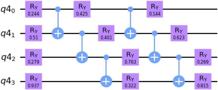
www.nature.com/scientificreports/
Boltzmann network efficiently, computing the exact model independent term in the training. Recently, Motta
et al.19 exploits the Quantum Imaginary Time Evolution (QITE) algorithm to determine eigenstates and thermal
states on a quantum computer. McArdle et al.20 showed how one could make use of variational circuits to cre-
ate states that represent the dynamics of the imaginary time evolution. They use it to compute the ground state
wavefunction of hydrogen and lithium hydride, while Yeter-Aydeniz et al.21 demonstrate that the QITE algorithm
serves as a quantum computing benchmark for computational chemistry methods.
Herein, we develop an optimization function using the method introduced by B urges22 and then use it as a
Hamiltonian to perform imaginary time evolution on a uniform superposition of all possible considered solu-
tions to the factorization problem. We employ variational circuits to prepare a quantum state that encodes the
solution and classically train all parameters. Simulations using Python Numpy packages and IBM-QASM are
used to verify the performance. The robustness of the techniques against noise is verified on IBMQ hardware for
up to 5 qubits allowing factorization of numbers up to 91 with a probability over 73%. To the best of our knowl-
edge this is the largest number that has been factorized on a quantum circuit using a general purpose algorithm
that does not exploit any structural properties of the number. Each iteration involves evaluating a number of
circuits that scales as O(n5 d) where n is the bit-string length of the number to be factorized and d is the circuit
depth. A few reasons make factorization an ideal candidate to be solved using Imaginary time evolution with
variational circuits. The number of terms in the Hamiltonian expansion scales polynomial with respect to the
number of qubits. The amplitude of coefficients in the state vector is real, which simplifies the parameterization
of the landscape to be explored and updates to be made. Each iteration only needs to amplify the amplitude of
the solution rather than exactly simulate the imaginary time evolution. These factors make Variational QITE a
good algorithm to be studied in the context of optimization, and make prime factorization a good test bed to
evaluate its working. We are hoping that future rigorous work along these lines, with the availability of more less
noisy qubits, might provide for ways in which this method complements with VQE for general optimization
problems approached using variational methods.
Background
The Schrödinger equation for a closed system describes dynamics according to some Hamiltonian that governs
it. Allowing for time to be complex, we are able to create thermal states of specific temperature starting from a
maximally mixed configuration, i.e, ρT=1/τ = e−Hτ /Tr[e−Hτ ]. Preparing a system at low temperature or alter-
natively letting the system evolve to large imaginary time values we can more often sample the ground state
configuration for a given Hamiltonian. We shall make use of this property to encode the required solution of
the problem we intend to solve in the later sections.
The quantum state we intend to prepare using QITE is given by,
|ψ(τ )� = N(τ )e−Hτ |ψ(0)� (1)
where N(τ ) = 1/ �ψ(0)|e−2Hτ |ψ(0)� is a normalization factor. Equation (1) satisfies the Wick rotated Schro-
dinger equation
∂|ψ(τ )�
= −(H − Eτ )|ψ(τ )� (2)
∂τ
where Eτ = �ψ(τ )|H|ψ(τ )�.
Let |φ(τ )� be a state that is prepared by applying a series of unitary gates as follows
|φ(τ )� = UN (θN )UN−1 (θN−1 )UN−2 (θN−2 )UN−3 (θN−3 ) . . . U1 (θ1 )|0� (3)
We choose the initial parameters to create the state on which the evolution is to be performed. We demand that
Eq. (3) is an approximate solution to Eq. (2) by demanding the norm of the variation to vanish, i.e,
∂
δ
+ H − Eτ |φ(τ )� = 0 (4)
∂τ
Solving the above equation using McLachlan’s variational principle (see Supplementary section 1 for proof) we
obtain
Aij θ˙j = Ci (5)
where
∂�φ(τ )| ∂|φ(τ )�
Aij =
∂θi ∂θj
(6)
∂�φ(τ )|
Ci = − H|φ(τ )�
∂θi
The derivatives on the state vectors with respect to the parameters of the circuit can be simplified into a sum of
other basic circuit functions. For instance, the derivative of the Rx , Ry and Rz rotation gates with respect to their
parameter amounts to a mere shift of the parameter by an angle of π radians. We can further express H as a sum
of a string of tensor products of Pauli operators allowing both A and C to be computed as the sum of terms that
take the form aR(eiφ �0|U|0�), where a is some real number and φ is a real phase. Terms of this form can be
efficiently computed on quantum hardware using the Hadamard test.
Scientific Reports | (2021) 11:20835 | https://doi.org/10.1038/s41598-021-00339-x 2
Vol:.(1234567890)
www.nature.com/scientificreports/
Evaluating the gradients using Eq. (5), we can then proceed to use gradient descent to update the parameters
of the circuit as follows
� ) + θ�˙ (τ )δτ
� + δτ ) = θ(τ
θ(τ (7)
�˙ ) = A−1 (τ )C(τ ). Using sufficient layers to the variational circuit and small δτ time iterations for
where θ(τ
updating our parameters, we can prepare states that closely emulate the imaginary time evolution on the state
|ψ(0)�. We would like to note that the dynamics of ITE is non unitary and thus we are only able to prepare the
output state starting from a fixed initial state using variational methods.
Methods
The problem of prime factorization involves expressing a number as a product of its primes. Here we shall focus
specifically on biprimes, product of 2 prime numbers. Shor’s algorithm aims to solve this problem by reducing
it to a period finding problem of the function ax mod N, where a is any random number and N is the number to
be factorized. This algorithm uses a quantum subroutine that exploits the power of quantum Fourier transform
as a part of a modified phase estimation algorithm. The largest number factorized using Shor’s algorithm is 21.
Being highly sensitive to discrete errors, Shor’s algorithm fails to scale without viable error correction s chemes23.
Here we show how to factorize a given number by first casting it as an optimization problem. Let the number
N be given by a product of 2 prime numbers p and q. We model the problem of finding p and q given N as an
optimization problem cast as the following cost function
H(p, q) = (N − p × q)2 (8)
Note that in Eq. (8), H(p, q) has global minima when p,q factorize N with a minimum value of 0. The cost function
can thus be treated as a Hamiltonian whose ground state encodes the solution to our problem. We express both
p and q as a binary string summation which will allow us to transfer to a qubit representation space. Assuming
p has an m bit representation and q has an l bit representation, we get
p = 2m−1 pm−1 + 2m−2 pm−2 . . . 20 q0
(9)
q = 2l−1 ql−1 + 2l−2 ql−2 . . . 20 q0
Note that Eq. (8) has a trivial solution N = N × 1. To exclude this solution, we can restrict the search space
of our solution by using a lower bound. The smallest prime factor we are looking for is greater than 2 and less
than N/2. Thus using N − 1 qubits to represent p and q we can discard the trivial solution from showing up in
our simulation. Since both p and q are prime numbers, we are allowed to set the bit 0 to be 1 in either expres-
sion making it indivisible by 2. To move to a scaled spin representation we transform all the binary variables
bi that represents either the pi ’s or qi ’s to bi = (si + 1)/2. In this representation, si takes the value ±1 such that
si = 1 maps to bi = 1 and si = −1 maps to bi = 0. We thus convert a factorization problem into an optimization
problem over the spin variables.
Minimizing this optimization function shall result in the solution we seek. We use imaginary time evolution
to evolve the output state starting from a uniform superposition over all possible solutions at T = 0. The circuit
parameters are updated according to Eqs. (5) and (7). With every iteration that is performed, the output state
evolves through a time step of δτ . After sufficiently large enough time T, we expect the ground state with the
least cost to prepare. For ||H||1 T >> 1 we get,
e−HT |+ + · · · +� ≈ p̃ q̃ (10)
where p̃ and q̃ represent the bit string solution of the binary representation of the numbers that multiply to give
N. The evolution is achieved by using a variational circuit ansatz to prepares states that mimic the evolution of the
system from a given starting state (as described in the previous section). The computational cost in performing
one iteration of QITE is O(n5 d), where n is the bit-length of the number to be factored and d is the depth of the
circuit (see Supplementary section 2 for proof).
Here we show an example of how to factorize N = 15 as
15 = 5 × 3 (11)
Expressing the factors 5 and 3 as binary variables and setting p0 = 1, q0 = 1 yields
5 = 4x1 + 2x0 + 1
(12)
3 = 2x2 + 1
with the correct results defined by x0 = 0, x1 = 1, x2 = 1. The corresponding cost function H(p, q) is cast as
H(x0 , x1 , x2 ) = [15 − (4x1 + 2x0 + 1)(2x2 + 1)]2 (13)
Expanding the cost function and making use of xi2 = xi yields,
H(x0 , x1 , x2 ) = 196 − 52x2 − 52x0 − 56x2 x0 − 96x1 − 48x2 x1 + 16x0 x1 + 128x0 x1 x2 (14)
Mapping the binary variables to spin variables yields,
H(s0 , s1 , s2 ) = 90 − 36s2 − 40s1 − 20s0 + 2s2 s0 + 4s2 s0 + 20s0 s1 + 16s0 s1 s2 (15)
Scientific Reports | (2021) 11:20835 | https://doi.org/10.1038/s41598-021-00339-x 3
Vol.:(0123456789)www.nature.com/scientificreports/
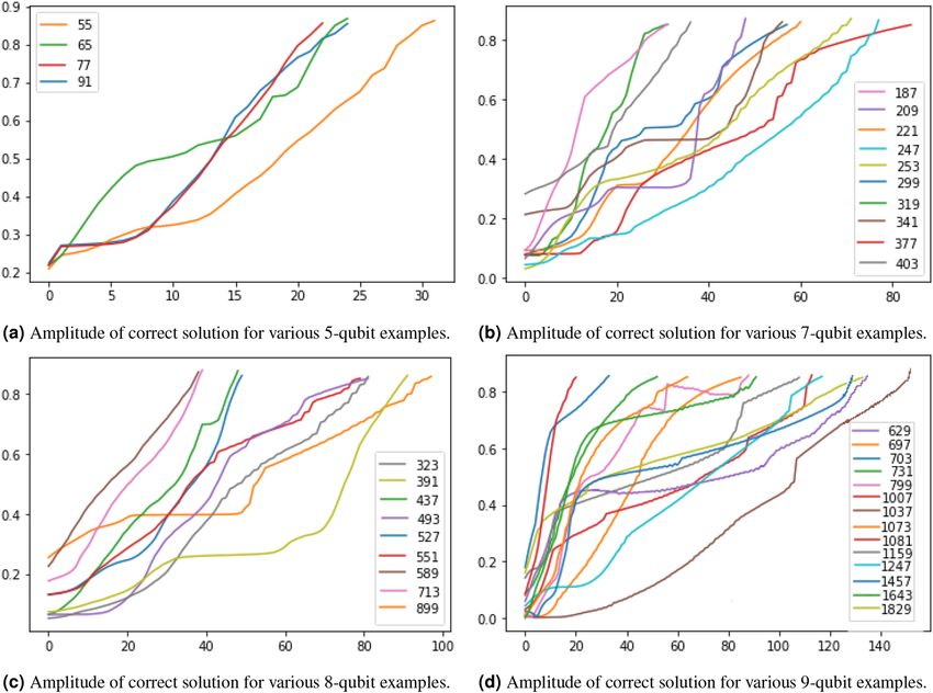
Figure 1. Variational circuit used to prepare the quantum state for imaginary time evolution. The parameters
have been randomly initialized.
The classical binary variables si in the Hamiltonian is replaced by the Pauli-z spin operator to get a quantum
Hamiltonian Operator that is then acted upon the full superposition state. Using a time step δτ = 0.1 , we make
10 iterations of QITE to reach T = 1. When simulated on QISKIT Aer using state-vector simulator backend,
with a probability of greater than 90%, we obtain upon measurement
e−HT |+ + +� ≈ |110� (16)
where the above expression is written in the computational basis. The output Eq. (16) when mapped back to the
binary variables gives
x0 = 0, x1 = 1, x2 = 1 (17)
We thus obtain the factors of 3 and 5 as expected. In our simulations, we shall make use of no more than the
number of qubits needed to represent our solution in the optimization. This is to limit the numbers of qubits
used, maximize the computational efficiency and reduce the accumulated errors.
We generate the output quantum state prepared using QITE with the ansatz shown in Fig. 1. Notice that the
circuit consists of RY rotation gates applied to each qubit followed by a layer of CNOT gates that help with the
entanglement of the qubits. Using only RY gates ensures that we maintain real amplitudes for the state when
expressed in the computation basis. This helps with closely following the dynamics of QITE without introducing
any nontrivial phase values.
Equation (5) for such a circuit ansatz can be re-expressed in terms of the quantum Fisher information (QFI)
and the gradient of Hamiltonian expectation with respect to the current state. In classical probability, the Fisher
information characterizes how much a probability distribution varies by changing a parameter that characterizes
a distribution. This can be generalized and extended to talk about quantum states where one characterizes how
much a state changes with respect to the parameter that governs it. Refer24 for a brief introduction to quantum
Fisher information. Given a quantum state |ψ(θ1 , θ2 . . . θn )�, where θi represents the governing parameters, the
QFI is given by
Fij = 4R(�ψi |ψj � − �ψi |ψ��ψ|ψj �) (18)
d |ψ(θj )�
where ψj = dθ . For the ansatz being used to generate the state in QITE, we note that �ψi |ψ� = R(�ψi |ψ�).
This results in the second term vanishing due to the constant normalization of the state i.e, �ψ|ψ� = 1. Hence we
get Fij = 4Mij where Mij = R(�ψi (θ(τ ))|ψj (θ(τ ))�). Note Fij being real symmetric, avoids the unstability that
is likely to occur from inverting a skew symmetric matrix with small imaginary coefficients. Furthermore, since
the Hamiltonian is an Hermitian operator, we can express the right hand side of Eq. (5) as follows
d
Ci = R(�ψ|H|ψi �) = (�ψ|H|ψ�)/2 (19)
dθi
We thus obtain j Fij θ˙j = −2 dθd i �H�ψ . The QFI of a given circuit and the gradient of an observable with respect
to a state parameter can be directly computed in the IBM Qiskit Aqua framework (see Supplementary section 3
for QFI module).
Results
Simulations. Smaller numbers were factorized on Qiskit using the QASM simulator. For 8 qubits and more,
the simulations were run using the Numpy package. The amplitude threshold for the correct solution has been
set to 0.85, this amounts to a probability of 73% to get the right solution when measured in the computational
basis. We have restricted our ansatz to a single layer in addition to the base layer, in light of exploring shallow
circuits for the near term quantum computers. The initial circuit parameters have been randomly sampled to
help avoid valleys during the training and allow for faster convergence with shallow circuits employed. We have
noticed that it also helps in suppressing one of the solutions in the case of symmetrically equivalent solutions
(for instance, 391 can be factorized as 17 × 23 and 23 × 17), allowing one solution to quickly reach the threshold.
Figure 2 plots the amplitude of the solution in the computational basis against the number of iterations for sev-
Scientific Reports | (2021) 11:20835 | https://doi.org/10.1038/s41598-021-00339-x 4
Vol:.(1234567890)www.nature.com/scientificreports/
Figure 2. Numerical simulations of QITE for 7-, 8-, and 9-qubit factorization examples. The vertical axis
indicates the amplitude of the solution in the computational basis and the horizontal axis indicates the number
of iterations made. The curves in each subplot show how the amplitude of the solution corresponding to various
numbers increases with iterations. The amplitude threshold has been set to 0.85.
eral values of N that are represented using 5, 7, 8, and 9-qubit Hamiltonians. Note the amplitude of the solution
to the factorization keeps raising with increasing the number of iterations. The figure also shows that the average
number of iterations required to factorize increases with the number of qubits though we have not been able to
analytically bound it. A few instances involve the amplitude of the solution flattening before continuing to raise
any further, making it significantly slow. In Table 1, we note that despite some numbers being close to each other
(for instance 1007 and 1081), the number of iterations for convergence to the solution seem to be widely varying.
This can be attributed to the differences in bit string representation and thus the point of minima to the created
cost function, and also to the fact that the parameters are being randomly initialized. Results on actual hardware
for smaller instances have been presented in the next subsection. We have tested this method against a standard
Variational Quantum EigenSolver (VQE), and would like to note that no statistically significant difference with
regards to the number of iterations for converging to the solution has been observed.
Results on IBM‑Hardware. We have made use of the publicly available IBM hardware to simulate factori-
zation for up to 5 qubits. We start the output state with a uniform superposition over all possible solutions. This
is straightforwardly instantiated by setting the parameters of Ry gates in the base layer to be π2 and the remaining
parameters to be all 0. We have avoided invoking the Hadamard test to compute the M matrix and C vector as
this resulted in significant error accumulation. Instead, we have reformulated the computation as indicated in
the methods section and have made use of built-in Qiskit modules. The Gradient module with parameter shift
method has been used to compute the C vector, while the QFI module with overlapping block diagonal method
has been used to compute the M matrix. The built in QFI module makes 1024 shots on every circuit to be evalu-
ated and includes no measurement error mitigation by default. Please refer to the Qiskit source documentation25
for details on the implementation of these modules. Figure 3 shows the results of factorizing the numbers N =
55, 65, 77 and 91 on IBMQ-lima hardware that supports 5 qubits. Unlike the simulations that hardly show any
oscillation in the amplitude, we see oscillations being introduced due to noise when run on the hardware. The
convergence of the solution in the presence of hardware noise makes this method a suitable candidate for solving
factorization and other similarly framed optimization problems in the near term quantum computers.
Scientific Reports | (2021) 11:20835 | https://doi.org/10.1038/s41598-021-00339-x 5
Vol.:(0123456789)www.nature.com/scientificreports/
Number factorized Number of iterations
55 31
65 23
77 21
91 23
187 30
209 48
221 61
247 77
253 72
299 58
319 30
341 57
377 84
403 36
323 81
391 89
437 48
493 80
527 47
551 77
589 38
629 132
697 59
703 31
713 39
731 56
799 86
899 96
1007 21
1037 155
1081 112
1159 103
1247 112
1457 128
1643 88
1829 130
Table 1. Table lists the numbers that were factorized alongside the number of iterations for convergence.
Discussion
We have shown how imaginary time evolution can be used to perform optimization and have demonstrated this
for the case of prime factorization. We have shown numerical and experimental results from the factorization of
several numbers represented by 7, 8, and 9-qubit Hamiltonians. We have shown that imaginary time evolution
significantly populates the probability of measuring the correct solution to the factorization problem when run
sufficiently long. The observed performance of the method on the IBM-lima hardware shows that the method is
robust to noise and works as a proof of concept in the case of a limited number of qubits. Future work towards
bounding the number of iterations analytically can help highlight the performance of this method against well
known factorization techniques. We hope that the results explored here promote future work in the direction of
exploring Quantum Imaginary time evolution in the context of solving optimization problems.
Scientific Reports | (2021) 11:20835 | https://doi.org/10.1038/s41598-021-00339-x 6
Vol:.(1234567890)www.nature.com/scientificreports/
Figure 3. 5-qubit factorization on IBMQ-lima. The vertical axis indicates the amplitude of the solution in
the computational basis and the horizontal axis indicates the number of iterations made. The curves in each
subplot, show how the amplitude of the solution corresponding to various numbers increase with iterations. The
amplitude threshold has been set to 0.85.
Received: 21 July 2021; Accepted: 24 September 2021
References
1. Bernstein, D. J. Introduction to Post-quantum Cryptography 1–14 (Springer, 2009).
2. Ambainis, A. Quantum search algorithms. ACM SIGACT News 35, 22–35. https://doi.org/10.1145/992287.992296 (2005).
3. Preskill, J. Quantum computing in the NISQ era and beyond. Quantum 2, 79. https://doi.org/10.22331/q-2018-08-06-79 (2018).
4. Dixit, V., Selvarajan, R., Alam, M. A., Humble, T. S. & Kais, S. Training and classification using a restricted Boltzmann machine
on the D-Wave 2000Q. Preprint arXiv:2005.03247 (2020).
5. Dixit, V. et al. Training a quantum annealing based restricted Boltzmann machine on cybersecurity data. IEEE Trans. Emerg. Top.
Comput. Intell.https://doi.org/10.1109/TETCI.2021.3074916 (2021).
6. Outeiral, C. et al. The prospects of quantum computing in computational molecular biology. WIREs Comput. Mol. Sci. https://doi.
org/10.1002/wcms.1481 (2021).
7. Sureshbabu, S. H., Sajjan, M., Oh, S. & Kais, S. Implementation of quantum machine learning for electronic structure calculations
of periodic systems on quantum computing devices. Preprint arXiv:2103.02037 (2021).
8. Cao, Y., Jiang, S., Perouli, D. & Kais, S. Solving set cover with pairs problem using quantum annealing. Sci. Rep. 6, 1–15 (2016).
9. Kais, S., Whaley, K., Dinner, A. & Rice, S. Quantum Information and Computation for Chemistry. Advances in Chemical Physics
(Wiley, 2014).
10. Brown, K. L., Daskin, A., Kais, S. & Dowling, J. P. Reducing the number of ancilla qubits and the gate count required for creating
large controlled operations. Quantum Inf. Process. 14, 891–899 (2015).
11. Shor, P. W. Polynomial-time algorithms for prime factorization and discrete logarithms on a quantum computer. SIAM J. Comput.
26, 1484–1509. https://doi.org/10.1137/s0097539795293172 (1997).
12. Vandersypen, L. M. K. et al. Experimental realization of Shor’s quantum factoring algorithm using nuclear magnetic resonance.
Nature 414, 883–887. https://doi.org/10.1038/414883a (2001).
13. Lucero, E. et al. Computing prime factors with a Josephson phase qubit quantum processor. Nat. Phys. 8, 719–723. https://doi.org/
10.1038/nphys2385 (2012).
14. Geller, M. R. & Zhou, Z. Factoring 51 and 85 with 8 qubits. Preprint arXiv:1304.0128 (2013).
15. Jiang, S., Britt, K. A., McCaskey, A. J., Humble, T. S. & Kais, S. Quantum annealing for prime factorization. Sci. Rep. 8, 17667 (2018).
16. Dattani, N. S. & Bryans, N. Quantum factorization of 56153 with only 4 qubits. arXiv:1411.6758 (2014)
17. Magnus, W. On the exponential solution of differential equations for a linear operator. Commun. Pure Appl. Math. 7, 649–673.
https://doi.org/10.1002/cpa.3160070404 (1954).
18. Shingu, Y. et al. Boltzmann machine learning with a variational quantum algorithm. Phys. Rev. A 104, 032413 (2020).
19. Motta, M. et al. Determining eigenstates and thermal states on a quantum computer using quantum imaginary time evolution.
Nat. Phys. 16, 205–210. https://doi.org/10.1038/s41567-019-0704-4 (2019).
20. McArdle, S. et al. Variational ansatz-based quantum simulation of imaginary time evolution. Quantum Inf.https://d oi.o
rg/1 0.1 038/
s41534-019-0187-2 (2019).
21. Yeter-Aydeniz, K. et al. Benchmarking quantum chemistry computations with variational, imaginary time evolution, and Krylov
space solver algorithms. Adv. Quantum Technol. 4, 2100012. https://doi.org/10.1002/qute.202100012 (2021).
22. Burges, C. J. Factoring as optimization. Tech. Rep. MSR-TR-2002-83 (2002).
23. Devitt, S. J., Fowler, A. G. & Hollenberg, L. C. Investigating the practical implementation of Shor’s algorithm. In Micro-and Nano-
technology: Materials, Processes, Packaging, and Systems II, Vol. 5650, 483–494 (International Society for Optics and Photonics,
2005).
24. Petz, D. & Ghinea, C. Introduction to quantum Fisher information. Quantum Probab. Relat. Top.https://doi.org/10.1142/97898
14338745_0015 (2011).
25. Abraham, H. & AduOffei. Qiskit: An open-source framework for quantum computing. https://doi.org/10.5281/zenodo.2562110
(2019).
Acknowledgements
We would like to thank Dr. Mario Motta and Dr. Stefan Woerner of IBM for useful discussion. We would like
to acknowledge the support from National Science Foundation under award number 1955907. This material is
based upon work supported by the U.S. Department of Energy, Office of Science, National Quantum Information
Scientific Reports | (2021) 11:20835 | https://doi.org/10.1038/s41598-021-00339-x 7
Vol.:(0123456789)www.nature.com/scientificreports/
Science Research Centers, Quantum Science Center. This manuscript has been authored by UT-Battelle, LLC,
under contract DE-AC05-00OR22725 with the US Department of Energy (DOE). The US government retains
and the publisher, by accepting the article for publication, acknowledges that the US government retains a
nonexclusive, paid-up, irrevocable, worldwide license to publish or reproduce the published form of this manu-
script, or allow others to do so, for US government purposes. DOE will provide public access to these results
of federally sponsored research in accordance with the DOE Public Access Plan (http://energy.gov/downloads/
doe-public-access-plan).
Author contributions
S.K., T.H. and X.C. designed the research problem, R.S. performed hardware testing and wrote the paper, R.S
and V.D coded for simulations using Python Numpy. All authors helped in revising the paper draft.
Competing interests
The authors declare no competing interests.
Additional information
Supplementary Information The online version contains supplementary material available at https://doi.org/
10.1038/s41598-021-00339-x.
Correspondence and requests for materials should be addressed to S.K.
Reprints and permissions information is available at www.nature.com/reprints.
Publisher’s note Springer Nature remains neutral with regard to jurisdictional claims in published maps and
institutional affiliations.
Open Access This article is licensed under a Creative Commons Attribution 4.0 International
License, which permits use, sharing, adaptation, distribution and reproduction in any medium or
format, as long as you give appropriate credit to the original author(s) and the source, provide a link to the
Creative Commons licence, and indicate if changes were made. The images or other third party material in this
article are included in the article’s Creative Commons licence, unless indicated otherwise in a credit line to the
material. If material is not included in the article’s Creative Commons licence and your intended use is not
permitted by statutory regulation or exceeds the permitted use, you will need to obtain permission directly from
the copyright holder. To view a copy of this licence, visit http://creativecommons.org/licenses/by/4.0/.
© The Author(s) 2021
Scientific Reports | (2021) 11:20835 | https://doi.org/10.1038/s41598-021-00339-x 8
Vol:.(1234567890)You can also read