Precise genotyping of circular mobile elements from metagenomic data uncovers human-associated plasmids with recent common ancestors - Genome Res
←
→
Page content transcription
If your browser does not render page correctly, please read the page content below
Downloaded from genome.cshlp.org on June 13, 2022 - Published by Cold Spring Harbor Laboratory Press

Method

Precise genotyping of circular mobile elements from
metagenomic data uncovers human-associated
plasmids with recent common ancestors
Nitan Shalon,1,2 David A. Relman,1,3,4 and Eitan Yaffe1,3
1
 Infectious Diseases Section, Veteran Affairs Palo Alto Health Care System, Palo Alto, California 94304, USA; 2Washington University
in St. Louis, St. Louis, Missouri 63130, USA; 3Department of Medicine, 4Department of Microbiology and Immunology, Stanford
University School of Medicine, Stanford, California 94305, USA

        Mobile genetic elements with circular genomes play a key role in the evolution of microbial communities. Their circular
        genomes correspond to circular walks in metagenome graphs, and yet, assemblies derived from natural microbial commu-
        nities produce graphs riddled with spurious cycles, complicating the accurate reconstruction of circular genomes. We pre-
        sent DomCycle, an algorithm that reconstructs likely circular genomes based on the identification of so-called “dominant”
        graph cycles. In the implementation, we leverage paired reads to bridge assembly gaps and scrutinize cycles through a nu-
        cleotide-level analysis, making the approach robust to misassembly artifacts. We validated the approach using simulated and
        real sequencing data. Application of DomCycle to 32 publicly available DNA shotgun sequence data sets from diverse nat-
        ural environments led to the reconstruction of hundreds of circular mobile genomes. Clustering revealed 20 highly prev-
        alent and cryptic plasmids that have clonal population structures with recent common ancestors. This method facilitates the
        study of microbial communities that evolve through horizontal gene transfer.

        [Supplemental material is available for this article.]

Horizontal gene transfer (HGT) is a major driver of microbial evo-                  edges represent contig–contig adjacencies supported by crossing
lution (Soucy et al. 2015). HGT supports the rapid adaptation of                    reads. One formulation of the problem at hand is the identification
microbes to ecological niches (Wiedenbeck and Cohan 2011;                           of circular graph walks that correspond to underlying circular ge-
Polz et al. 2013) and facilitates the spread of virulence factors                   nomes. Yet some circular walks are in fact “phantoms,” for which
and antimicrobial-resistance determinants within and between                        the corresponding circular genomes are not present in the biolog-
microbial species (Maiques et al. 2006; von Wintersdorff et al.                     ical sample. These phantom walks are a result of identical (or near-
2016; Deng et al. 2019). Extrachromosomal circular mobile genetic                   ly identical) DNA sequences appearing in different genomic
elements (ecMGEs), such as plasmids and phage with circular ge-                     contexts. Repeat elements such as transposons and integrated
nomes, are of particular interest as common agents of HGT                           phage are common in microbial genomes. Moreover, natural mi-
(Frost et al. 2005). Experimental methods have been developed                       crobial communities have been shown to simultaneously harbor
to genotype ecMGEs in complex microbial communities, includ-                        closely related ecMGEs that differ by only a few genome rearrange-
ing the physical enrichment of plasmids (Sentchilo et al. 2013)                     ments (Conlan et al. 2014; He et al. 2015; Suzuki et al. 2019).
and of viral particles (Shkoporov et al. 2018), and the removal of                  Repeats and rearrangements produce complex graphs riddled
linear DNA followed by multiple displacement amplification                          with phantom walks, complicating the task.
(Jørgensen et al. 2014). In the last decade, MGE characterization                         Several tools traverse the assembly graph in an attempt to re-
has been shifting toward the use of direct shotgun sequencing of                    construct complete genomes of ecMGEs (Rozov et al. 2017;
complex communities, owing to reduced cost and benchwork sim-                       Antipov et al. 2019; Pellow et al. 2021). These tools efficiently
plicity. Several tools scan shotgun metagenomic assemblies to                       search for circular graph walks that may correspond to ecMGEs,
identify MGE-associated sequences by searching for genetic signa-                   yet their heuristic nature makes them highly susceptible to errors.
tures of plasmids and phage (Zhou and Xu 2010; Lanza et al. 2014;                   A review estimated that >25% of ecMGE genomes reported by ex-
Carattoli et al. 2014; Roux et al. 2015; Roosaare et al. 2018;                      isting approaches do not correspond to true ecMGEs (Arredondo-
Robertson and Nash 2018). However, these tools do not recon-                        Alonso et al. 2017). Meanwhile, theory has been developed to for-
struct complete genomes and can conflate extrachromosomal                           mulate the correctness of walks in assembly graphs (Obscura
with integrated forms of mobile elements, confounding the study                     Acosta et al. 2018). However, theory revolving around the correct-
of ecMGEs in natural settings.                                                      ness of circular walks needed for the recovery of circular genomes is
      A powerful approach to recover complete genomes of ecMGEs                     lacking. The recovery of MGE genomes will allow the field to con-
is based on metagenomic assembly graphs. In these graphs, verti-                    duct high-throughput computational surveys of mobile elements,
ces represent contigs (partially assembled DNA sequences), and                      strengthening the understanding of the evolution and spread of
                                                                                    mobile elements and their genetic cargo in natural environments.

Corresponding authors: relman@stanford.edu,
eitanyaf@stanford.edu
Article published online before print. Article, supplemental material, and publi-   © 2022 Shalon et al. This article, published in Genome Research, is available un-
cation date are at https://www.genome.org/cgi/doi/10.1101/gr.275894.121.            der a Creative Commons License (Attribution 4.0 International), as described at
Freely available online through the Genome Research Open Access option.             http://creativecommons.org/licenses/by/4.0/.

32:1–18 Published by Cold Spring Harbor Laboratory Press; ISSN 1088-9051/22; www.genome.org                                        Genome Research                1
                                                                                                                                      www.genome.org
Downloaded from genome.cshlp.org on June 13, 2022 - Published by Cold Spring Harbor Laboratory Press
Shalon et al.
The goal of this work was to develop a tool (DomCycle) sult in the same graph. This is illustrated by two manufactured
that reliably infers circular genomes of ecMGEs from short-read configurations (Fig. 1A,B) and the graph that corresponds to
shotgun DNA data derived from complex microbial communi- both (Fig. 1C). To simplify the problem, we focused on cycles,
ties. A second goal was to validate DomCycle using negative con- which are circuits that do not include any contig more than
trols without circular genomes, reference ecMGE data, and once. Yet, even cycles may have no true corresponding genome.
realistic simulations of evolving mobile elements. A final goal Repeat elements can result in spurious cycles (called here “phan-
was to showcase the discovery potential of DomCycle by apply- tom” cycles) for which no corresponding circular genome exists
ing the tool to metagenomic data generated from diverse micro- in one or more of the possible latent genome configurations (illus-
bial communities. trated in Fig. 1C). Our goal was to develop a tool that calculates ro-
bust mathematical attributes of cycles that can help distinguish
between phantom and real cycles.
Results
We developed a theoretical framework and associated tool
(DomCycle) to recover near-complete genomes of ecMGEs from Algorithm that recovers all dominant graph cycles
metagenome assembly graphs (Fig. 1). In the assembly graph, cir- Our approach is based on a new concept called “dominant cycles.”
cuits are circular walks that correspond to circular chains of contigs. Dominant cycles are loosely related to the previously introduced
Although every circular genome produces a corresponding circuit notion of “dominant plasmids” (Antipov et al. 2019), yet they
in the graph, inferring the underlying genomes from the graph is are grounded in graph theory. We assume a latent configuration
nontrivial, as different underlying genome configurations can re- of circular genomes that produces an assembly graph (see
A Configuration B Alternative configuration
p1 p1
p2
10×
10×
p5
6×
p4 6×
p3 p4
3×
3×
18×
C D E
Assembly graph Candidate cycles Vetted cycles
10× 6×
c2
nt-level vetting
6× / 6×
c1 10× / 0×
Graph pruning
6× 6× c1
12×
10×
6× c3 6× ~24×
6× / 24×
~10×
18× 24× 18×
3×
3× c4 18× / 9×
~21× c4
21× 18×
c5 3× / 18×
3× 18×
3× ~18×
3×
Figure 1. Approach overview. (A) A manufactured example of a latent genome configuration and assembly with eight unique contigs. Contigs are color-
coded, and four DNA genomes are marked p1–p4 with their x-coverage specified in their center. For example, p2 has an x-coverage of 6× and contains only
three unique contigs, as the short purple contig appears twice. The corresponding assembly graph is shown in C. Under this configuration, cycle c4 is a real
cycle that corresponds to p3. (B) An alternative genome configuration that produces the same graph. The presence of the complex genome p5, which
corresponds to an involved circuit in the graph, affects the multiplicity of all visited cycles. For example, the multiplicity of cycle c4 is equal to four because
the circuit that corresponds to p5 visits the red contig four times while traversing in a loop along the contigs of c4. Note that under this configuration, cycle
c4 is a phantom cycle. (C) The assembly graph that corresponds to the configurations shown in A and B. Directed edges appear within a single contig (going
from the 5′ end to the 3′ end, represented with arrows) and between adjacent contigs (going from the 3′ end to the 5′ end, represented with dotted lines).
The graph contains five cycles (c1–c5), and the x-coverage of edges is indicated. (D) The cycle score σc/τc is specified in the center of each cycle for the graph
shown in C. The algorithm recovers all candidate dominant cycles (σc/τc > 1; score colored black) and discards nondominant cycles (score colored gray). For
example, cycle c4 has a score of two (σc = 18 × , τc = 9 × ), making it a candidate dominant cycle. (E) In our implementation, nucleotide-level read profiles are
computed for all candidate dominant cycles using all paired reads for which at least one side mapped to the cycle, and the algorithm returns dominant
cycles with estimates of x-coverage. Reads are grouped into cycle-supporting reads (black line) and nonsupporting reads (red line). For example, the x-
coverage of supporting reads along c4 varies, with three short stretches of nonsupporting reads on contig–contig seams. Average read x-coverage values
for portions of the cycles are shown on the plot.
2 Genome Research
www.genome.orgDownloaded from genome.cshlp.org on June 13, 2022 - Published by Cold Spring Harbor Laboratory Press
Precise genotyping of circular mobile elements
Methods). For every cycle c in the graph, the bottleneck coverage σc is this data set in 7 h, displaying similar performance as existing tools
the minimal read coverage along the edges of the cycle, the external (Supplemental Fig. S2).
coverage τc is the total number of paired reads leading in or out of We evaluated the performance of DomCycle on 100 reference
the cycle (averaging in and out), and the cycle score is the ratio σc/τc plasmids and 100 reference phage genomes, all assayed individual-
(Fig. 1D). We call a cycle dominant if σc/τc > 1. ly (Supplemental Table 2). Recall was 47% for plasmids and 91%
We also define two latent variables. Our latent variable of in- for phages, slightly lower than the maximal performance of the
terest is the coverage ψc of the genome associated with a cycle c (ψc other tools (Fig. 2D). DomCycle had near-perfect precision (Fig.
≥ 0 by definition and ψc = 0 if the genome is not part of the config- 2E) and consistently reported only a single cycle (or no cycle at
uration). A second latent variable is the multiplicity μc, which is all), whereas all other tools occasionally split a single genome
equal to the number of times the contigs of the cycle appear con- into multiple reported elements (Fig. 2F). Recall and precision
secutively within the context of a larger circuit, such as within a were robust to changes in key thresholds, such as the score cutoff
tandem repeat (defined in the Methods). For clarity, we emphasize that defines dominant cycles (Supplemental Fig. S3). We com-
that the last and possibly incomplete pass along the contigs of the pared all tools on a data set derived from a real microbial commu-
cycle is counted toward the multiplicity, as shown in Figure 1B. nity (CAMI) (Sczyrba et al. 2017) that included 40 genomes and 20
Our main theoretical result is the bound σc − μc × τc ≤ ψc. This lower ecMGEs (Fig. 2G). Again, DomCycle was precise at the expense of
bound on ψc means that either any dominant cycle is real (i.e., ψc > sensitivity (Fig. 2H). To summarize, DomCycle effectively limits re-
0) or it has a multiplicity greater than or equal to the cycle score porting phantom cycles while achieving recall values that are only
(i.e., σc/τc ≤ μc). Although high-multiplicity cycles are theoretically slightly inferior to existing tools.
possible, they require complex tandem structures as shown in
Figure 1B, and it is not clear how common they are in microbial ge- Validation using simulated mobile element data
nomes. To gauge the prevalence of high-multiplicity cycles that
We simulated two realistic scenarios of evolving mobile genetic el-
are dominant and phantom (called dominant-phantom), we
ements. The first scenario involved a single plasmid (central allele)
used empirical data, presented below.
and several variant plasmids (variant alleles) that were individually
We developed an algorithm that recovers all dominant cycles
distinguished from the major allele by a single-genome rearrange-
in an assembly graph. In the implementation of the algorithm,
ment event (insertion, deletion, or inversion). The second scenario
contig–contig edges in the assembly graph are inferred using
simulated a semi-induced prophage. It involved a phage that both
paired reads while bridging possible small gaps (for details, see
appeared in a circular form (central allele) and integrated several
Methods). Candidate cycles are vetted on a nucleotide-level basis
times into a linear genome (variant alleles). For both scenarios,
by comparing the ratio between the number of supporting reads,
we tested recall and precision as a function of the frequency of
for which both sides map with proper orientations to the cycle,
the central allele (Fig. 3A). Central alleles were recovered when
and the number of nonsupporting reads (Fig. 1E). This makes
the allele frequency surpassed 45% for plasmids and 55% for phag-
the approach robust to common forms of misassembly. Stochastic-
es. Despite a background of convoluted genome rearrangements,
ity in read coverage is modeled using a binomial distribution to
the precision was perfect in all cases; that is, all cycles reported
identify vetted dominant cycles with scores that are significantly
by DomCycle were associated with real underlying genomes, and
larger than one. We note that DNA replication (Antipov et al.
multiple cycles were never reported. To illustrate the performance
2016) and sequencing biases (Sato et al. 2019; Browne et al.
of DomCycle, we show the underlying graph cycle (Fig. 3B)
2020) introduce systematic biases to read coverage, which poses
and the distribution of mapped reads along the cycle (Fig. 3C)
a challenge to our assumption of uniform coverage. The algorithm
for a single successful plasmid run. In comparison, Recycler and
yields near-complete circular genomes (not necessarily complete
metaplasmidSPAdes had some precision issues, with Recycler
owing to possible small gaps between consecutive contigs) that
showing a minimum precision of 0% and metaplasmidSPAdes
correspond to all vetted dominant cycles.
achievingDownloaded from genome.cshlp.org on June 13, 2022 - Published by Cold Spring Harbor Laboratory Press
Shalon et al.
A B C
1k
1m
False-Positive Length
Bottleneck Coverage
212
100
False-Positive Count
100 100k
25
13 10k
10
10
1k
2
0 0 r r
10 100 1k 10k cle es cle PP cle es cle PP
Cy PAdecy SCA Cy PAdecy SCA
Non-support m S R m S R
Do mp D o mp
coverage
D E F
Plasmids Phage Plasmids Phage Plasmids Phage
100 100 100
75 75 75
% Samples
% Precision
% Recall
50 50 50
25 25 25
0 l id h 0 l id h 0 d l d l
cle es ler PP cle es ler PP cle es ler PP ycle des cler PP + 1 + 1 + 1 + + 1 + 1 + -1 +
0 -1 2 0 - 2 0 - 2 0 - 2 0 -1 2 0 - 2 0 - 2 0 2
Cy Ad yc A Cy Ad yc A Cy Ad yc A C A y A DC mpS Rec SCA DC mpS Rec SCA
om SP Rec SC om SP Rec SC om SP Rec SC om SP Rec SC
D m p D m p D m p D mp
# Cycles Reported Per Sample
G H
DomCycle SCAPP
100 100
Recycler 0 0 mpSPAdes
0 75 75
0 0
% Precision
% Recall
0 0 0 0 50 50
11
0 0 25 25
1 5
0 0
2 r
r
cle es le PP cle es le PP
Cy PAd cyc SCA Cy Ad yc A
m S e om pSP Rec SC
R
Do mp D m
Figure 2. Specificity and sensitivity estimated with reference sequences. (A) The distribution of the bottleneck coverage versus the total nonsupport cov-
erage among cycles inspected by DomCycle on a metagenomic data set simulated on 155 reference chromosomal sequences. The dashed line shows the
threshold of significance (P < 0.01) for the global nucleotide test. Three cycles had global scores significantly above one and were selected as candidate
dominant cycles. (B) The number of phantom cycles reported on the simulated metagenomic data set, comparing the performance of DomCycle,
metaplasmidSPAdes (denoted by mpSpades), Recycler, and SCAPP. Two candidate dominant cycles passed the local nucleotide test. (C) The length dis-
tribution for phantom cycles reported on the simulated metagenomic data set. The two phantom cycles reported by DomCycle areDownloaded from genome.cshlp.org on June 13, 2022 - Published by Cold Spring Harbor Laboratory Press
Precise genotyping of circular mobile elements
A B
×
C D
×
×
Figure 3. DomCycle performance on recombining plasmids and partially induced phage. (A) The recall (red) and precision (blue) for simulations at vary-
ing central allele frequencies. Each point represents the results of 30 trials at a single central allele frequency. Central allele frequency was calculated as the
percentage of the total x-coverage contributed by the central allele. (B) Example of a recovered central allele plasmid with a frequency of 55%. Shown is a
subset of the assembly graph focusing on a single reported cycle. The graph is represented as in Figure 1C. The recovered cycle is colored in red, and ad-
jacent graph edges that are not part of the cycle are colored in gray. Coverage units show the edge coverage, W(e). Labels on internal edges show contig
names. (C) The nucleotide-level cycle coverage profile corresponding to the cycle depicted in panel B. The coverage of cycle supporting reads is colored in
black, and the coverage of nonsupporting reads is colored in red. (D) Median coverage, lower bound coverage, and adjusted median coverage (AMC) as
predictors of true allele frequency. The Pearson correlation coefficient (denoted with “r”) and root mean squared deviation (denoted with “e”) are shown
for each predictor. In each small cross, the horizontal line shows the median metric value of an estimator at a given central allele frequency, and the vertical
line depicts the interquartile range of the estimator, created with 30 replicates for each allele frequency. Diagonal dotted lines show the true central allele
frequency.
single contig, 13% were self-loops that included a small assembly that the low precision of current tools confounds the analysis of
gap that was bridged using paired reads, and the remaining 19% real data (Supplemental Fig. S10). Furthermore, cycles reported
of genomes spanned multiple contigs. We offer an example of a only by metaplasmidSPAdes had low scores that were close to
putative phage (Fig. 4A) and a putative plasmid (Fig. 4B; all one, supporting the possibility that many of them are in fact phan-
ecMGEs are shown in Supplemental Fig. S8). Of note, among the tom cycles (Supplemental Fig. S11).
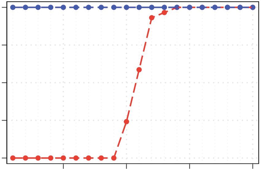
recovered ecMGEs was a complete genome of a member of the The AMC of the 49 ecMGEs ranged from 8.8× to 25,960× and
crAssphage family (Dutilh et al. 2014), a group of prevalent was on average 10-fold higher than the average coverage of all con-
Bacteroides phage (Supplemental Fig. S9). tigs in the assembly (Fig. 4D). This suggested that the detected
We applied metaplasmidSPAdes and SCAPP to the same gut ecMGEs have elevated abundance levels compared with the aver-
data set (Recycler did not complete the analysis within a week age abundance of bacterial members in the microbial community.
and was excluded). DomCycle and metaplasmidSPAdes were gen- However, to properly interpret AMC values, one needs to take into
erally in agreement, whereas SCAPP reported only three ecMGEs account the reduced probability of detecting low-coverage cycles
that clustered separately (Fig. 4C). The number of ecMGEs identi- owing to the stringent cycle vetting procedure. We computed for
fied by metaplasmidSPAdes and SCAPP was similar to their expect- each ecMGE its abundance percentile (AP), defined as the percentile
ed rate of false-positives (computed based on Fig. 2B), suggesting of its AMC score within a background distribution of AMC values
Genome Research 5
www.genome.orgDownloaded from genome.cshlp.org on June 13, 2022 - Published by Cold Spring Harbor Laboratory Press
Shalon et al.
A
B
C
D E
×
×
Figure 4. ecMGEs in the gut of a healthy adult. (A) A putative gut phage. Shown from inner to outer circles are nucleotide-level coverage profiles,
UniRef100 hits (sequence identity [AAI] to the best UniRef100 hit and the number of UniProt genes in the UniRef100 cluster), and gene classification.
Gene descriptions for select phage-associated genes are specified outside. Cycles are cut open at the start of their linear sequence for visualization purposes.
(B) Same as A, for a putative plasmid. (C) Genomes corresponding to reported cycles pairwise aligned and clustered using a threshold ANI of 95%. Shown is
cluster breakdown for DomCycle, metaplasmidSPAdes, and SCAPP. (D) Shown are the empirical cumulative distribution functions (ECDFs) for the AMC of
the 49 vetted dominant cycles that correspond to putative ecMGEs (black), the background AMC defined as the AMC of contigs vetted in the same way as
dominant cycles except for the circularity condition (dark gray), and the background coverage all contigs in the assembly (light gray). (E) Shown for all 49
vetted dominant cycles is the ECDF of the cycle abundance percentile, defined as the percentile of the cycle AMC within the background AMC distribution.
P-value computed using a one-sided Kolmogorov–Smirnov test is shown.
estimated using all contigs in the assembly (Methods). Even after 10−13), with 20 ecMGEs (41%) above the 95th AP (Fig. 4E).
this normalization, ecMGEs were significantly abundant within Analysis of shotgun data (96 million paired reads) derived from
the community (Kolmogorov–Smirnov test D = 0.543, P < 3.6 × the stool of a second healthy individual (Yaffe and Relman 2020)
6 Genome Research
www.genome.orgDownloaded from genome.cshlp.org on June 13, 2022 - Published by Cold Spring Harbor Laboratory Press
Precise genotyping of circular mobile elements
qualitatively recapitulated the elevated abundances of ecMGEs was 99.56%–100% (median 100%), and the average ANI within
(Supplemental Fig. S12). the aligned region was 98.43%–100% (median 99.9%). We refer
to these clustered ecMGEs, which were reconstructed indepen-
Comparing DomCycle to existing tools dently with minor genetic variations in multiple samples, as circu-
lating ecMGEs.
Recycler, the first tool that identified ecMGEs from assembly We classified 16 clusters as putative plasmids owing to the
graphs, uses a heuristic approach that results in limited precision presence of mobility and/or replication genes, of which five had
when applied to reference ecMGEs (Figs. 2E,H) and to realistic evo- one or two toxin–antitoxin genes, as summarized in Table 1 (for
lutionary scenarios (Supplemental Fig. S4). SCAPP, designed to ad- details, see Supplemental Table 5). There were 33 uncharacterized
dress the precision issues of Recycler by using genetic signatures of genes in total, which made up 32% of each cluster on average
mobile elements, has improved precision at the expense of sensi- (Supplemental Table 6). Clusters had two to nine ecMGE members
tivity. Despite SCAPP’s improved precision owing to its refer- (Fig. 6B), and all were from a single environment except cluster
ence-based approach, SCAPP may still report complex linearly M3, which was observed in both gut and sewage samples. The
inserted elements with mobile genes as demonstrated in Figure AP of circulating ecMGEs was high (mean AP of 92%), in agree-
2, B and C. ment with a commonly observed ecological association between
prevalence and abundance (Fig. 6C).
Circular mobile elements are abundant in diverse Leveraging a comprehensive plasmid reference database
environments (PLSDB, with over 26 k plasmids) (Galata et al. 2019), we identified
We applied DomCycle to 30 environmental shotgun libraries, in- seven clusters with near-identical reference hits (99.7% ANI on av-
cluding human stool (median 104 million reads per sample) (The erage) (Supplemental Table 7). This independent reconstruction of
Human Microbiome Project Consortium 2012), sewage wastewa- the circulating ecMGEs provided validation of our metagenomic
ter (median 48 million reads per sample) (Hendriksen et al. approach. Moreover, the PLSDB metadata informed us about the
2019), and the marine environment (median 37 million reads putative host-range and environments of some of our clusters.
per sample; 10 samples each) (Supplemental Table 3; Biller et al. These data suggested that our circulating ecMGEs may have a
2018). In total, we identified 720 dominant cycles and reconstruct- broad host-range, with five (out of six with host data) associated
ed their associated ecMGE genomes. Analysis was limited to 221 with multiple taxonomic families (Table 1). We discovered that
ecMGEs (29%) that were at least 1 kb long (Fig. 5A). All ecMGEs the top three plasmids (M1–M3) were reported as cryptic
were classified based on annotations of predicted genes, as puta- Bacteroides plasmids in the 1980s (Wallace et al. 1981; Sóki et al.
tive plasmids (28%), putative phage (17%), unspecified mobile el- 2010). On the other hand, the 13 circulating ecMGEs that did
ements (17%), and undefined elements (38%) (Fig. 5B). The three not have a close reference in PLSDB (>95% ANI) despite their prev-
environments differed in the distribution of classes (chi-squared alence in the general population highlight the discovery power of
test P < 10−16), with the gut relatively depleted for undefined ele- our metagenomic approach.
ments, sewage enriched for plasmids and undefined elements, We proceeded to augment clusters with reference genomes
and marine samples enriched for undefined elements (Fig. 5C). (where available) and inferred cluster-specific phylogenic trees.
Recapitulating our observation in the two gut samples of Figure The most prevalent plasmid (M1; 4138 ± 10 bp long) was observed
4, the 221 recovered ecMGEs were highly abundant (KS-test P < in nine gut samples and had two isolate-based reference genomes
10−16), with 73% of ecMGEs above the 95th AP within their respec- (Fig. 6D). M1 is composed of a major clade (M1a; isolated previous-
tive communities. All ecMGE classes were associated to some de- ly from Bacteroides xylanisolvens) and a minor clade (M1b; isolated
gree with elevated abundance levels (Fig. 5D). Elevated previously from Bacteroides fragilis), with a genetic distance of
abundance of ecMGEs was observed in all environments yet was 3.27% separating the two inferred clade ancestors. Both have shal-
most prominent in the human gut (Fig. 5E). The high abundance low clonal trees distinguished by a handful of SNPs, with a mean
of ecMGEs we observed may be explained by high copy numbers, ANI of 99.95% and 99.76% between clade members for M1a and
preferential targeting of abundant microbial hosts, and/or promis- M1b, respectively. Out of the 12 gut samples we assayed, M1a
cuous ecMGE-host interactions. was present in seven out of 12 (58 ± 22%), making it one of the
most prevalent plasmids recorded in the human gut to date. A co-
alescence analysis suggests M1a has gone through a clonal expan-
Highly prevalent plasmids are rapidly circulating sion merely ∼600–1200 yr ago (Supplemental Note 4).
We were curious to see if we could find evidence of ecMGEs circu- Another cluster of interest is M18, a short cryptic plasmid
lating within and between environments. We therefore performed (1934 bp) recovered from two sewage metagenomic samples and
pairwise genome alignments of all 286 ecMGEs (>1 kb) detected in independently reconstructed from 17 isolates (primarily
the 32 environmental samples described in this work. A compari- Enterobacteriaceae species) that were collected across the globe
son of the fraction of the aligned region and the average nucleotide (Fig. 6E). The clonal population structure of M18 is in discordance
identity (ANI) within the aligned region suggested that ecMGEs with its host species, suggesting it is freely circulating between a
preferentially maintain their diversity through local mutations diverse set of hosts.
and not through large-scale genomic changes (Fig. 6A). The The remaining five ecMGE clusters that have reference ge-
ecMGEs were grouped into 244 clusters based on sequence identity nomes suggest that ecMGEs are found in diverse environments
using a threshold of 95% ANI (Supplemental Fig. S13). Results were and bacterial hosts (Supplemental Fig. S15). The nine ecMGE clus-
robust to changes in the clustering threshold (Supplemental Fig. ters with sufficient members to estimate their phylogeny had clon-
S14). Analysis was limited to the 20 clusters (denoted M1–M20) al populations with only 0%–3.2% putative recombined sites,
that had two or more members (Table 1; for cluster members, see suggesting recombination between circulating ecMGEs is relative-
Supplemental Table 4). Clusters were extremely tight; the average ly rare (Supplemental Fig. S16). Finally, we noted several examples
fraction of the aligned region between pairs of cluster members of clusters with an uneven distribution of SNPs along their
Genome Research 7
www.genome.orgDownloaded from genome.cshlp.org on June 13, 2022 - Published by Cold Spring Harbor Laboratory Press
Shalon et al.
A B C
D E
Figure 5. ecMGEs in the human gut, sewage wastewater, and marine environments. (A) The number of ecMGEs identified in each environment. (B) The
percentage of ecMGEs with assigned functional classes. (C) The percentage of ecMGEs within each environment, stratified by class. (D) The ECDF of abun-
dance percentile values of ecMGEs, stratified by class. (E) Same plot as in D, stratified by environment.
genomes, suggestive of possible adaptive evolution or recombina- The major limitation of the approach is that it recovers only
tion (Supplemental Fig. S17). circular genomes that correspond to dominant cycles. In reality,
some mobile elements are linear, and circular mobile elements
can contain repeat elements that produce circuits, both of which
Discussion would not be detected by our approach. Although linear extrachro-
We present an algorithm that recovers all dominant cycles in a mosomal DNA is outside the scope of this work, the ongoing tran-
metagenomic assembly graph and reconstructs their correspond- sition to long-read sequencing technologies will transform some
ing genomes. Our implementation achieves high precision by circuits to cycles. With meticulous handling of environmental
combining graph theory and nucleotide-level vetting of cycles. samples, long reads can extend up to 5–10 kb (Suzuki et al. 2019;
We show that in the context of microbial communities, dominant Moss et al. 2020). Combining long reads with the approach present-
cycles likely correspond to true extrachromosomal circular DNA. ed here will allow genotyping of complex ecMGEs, such as MGEs
Application to complex evolutionary scenarios and reference that contain insertion sequences (typically < 2.5 kb) and short trans-
data reliably recovers ecMGEs with a negligible false-positive rate. posons. Longer repeat elements and complex rearrangements that
8 Genome Research
www.genome.orgDownloaded from genome.cshlp.org on June 13, 2022 - Published by Cold Spring Harbor Laboratory Press
Precise genotyping of circular mobile elements
A B C
D
E
Figure 6. Analysis of circulating ecMGEs. (A) The distribution of cycle tightness metrics across pairs of ecMGEs (>1 kb) in the 32 samples assayed. The
overlap identity is defined as the average identity of aligned regions between two cycle genomes. The overlap fraction is defined as the percentage of two
cycle genomes that align. For a cycle pair, genomic similarity is defined as the overlap identity times the overlap fraction. Cycle pairs are linked if their ge-
nomic similarity is >0.95, and clusters are defined as groups of linked cycles. (B) The distribution of the number of members in clusters. (C) The ECDF of
abundance percentile values of circulating ecMGEs compared with ecMGEs stratified by their environment and with all ecMGEs. (D) Detailed view of cluster
M1. Data are projected onto a reference “pivot” cluster member (gut4, cycle 181) that is shown in a linear format for visualization purposes. Shown from
the bottom up are the x-coverage profiles of the pivot ecMGE member, SNP patterns of cluster members (in bold) and reference sequences (isolate source,
location, and year of collection), and annotated genes (on top). SNP patterns are colored according to differences from the pivot, with white indicating
segments that failed to align. A phylogenic tree is shown on the left. The units of the scale bar under the tree are mean nucleotide differences. Clades M1a
and M1b are marked on the plot. (E) Detailed view of cluster M18, represented as in D.
Genome Research 9
www.genome.org10
Shalon et al.
www.genome.org
Genome Research
Table 1. Clusters of extrachromosomal circular mobile genetic elements with two or more members, based on sequence identity
No. of No. of No. No. of
ID members Length Enviroment Identity AP Class genes uncharacterized Mobility Replication Addiction references Host family
M1 9 4148 Gut 98.27 0.999 Plasmid 8 4 MOBP1 Y T+A 2 Bacteroidaceae
M2 7 2751 Gut 98.97 0.998 Plasmid 2 1 MOBP1 3 Bacteroidaceae
Enterobacteriaceae
M3 4 4494 Gut, 99.92 0.939 Plasmid 8 4 NA Y T+A 6 Bacteroidaceae
sewage Moraxellaceae
M4 3 5820 Gut 99.94 1 Plasmid 9 5 MOBP1 Y T+A 0
M5 3 4971 Gut 99.7 0.947 Plasmid 8 2 MOBP1 Y T 0
M6 3 2413 Gut 98.86 0.366 Undetermined 4 3 NA 0
M7 2 3034 Gut 99.9 0.7076 Plasmid 2 0 MOBV Y 0
M8 2 2775 Gut 99.61 0.804 Plasmid 2 0 MOBV Y 1
M9 2 2750 Gut 98.4 1 Plasmid 2 0 MOBP1 Y 3 Pseudomonadaceae
Bacteroidaceae
M10 2 8598 Gut 99.52 0.837 Plasmid 11 5 MOBF 0
M11 2 5843 Gut 99.87 0.389 Plasmid 7 4 MOBP1 0
M12 2 1488 Sewage 100 0.408 Plasmid 2 1 NA Y 2 Enterobacteriaceae
M13 2 1483 Sewage 99.26 0.551 Plasmid 2 1 NA Y 0
M14 2 3086 Sewage 100 0.546 Plasmid 3 1 MOBQ 0
M15 2 1044 Marine 99.61 0.899 Undetermined 0 0 NA 0
M16 2 2585 Sewage 100 0.947 Plasmid 3 0 MOBV A 0
M17 2 2349 Sewage 99.91 0.536 Plasmid 2 0 MOBP1 Y 0
M18 2 1934 Sewage 99.95 0.389 Plasmid 2 1 NA Y 17 Enterobacteriaceae
Yersiniaceae
M19 2 1382 Sewage 100 0.613 Plasmid 2 1 MOBT Y 0
M20 2 1705 Sewage 98.22 0.482 Plasmid 1 0 NA Y 0
Table columns from left to right specify for each cluster the number of cluster members, the average genome length in base pairs, the environments in which the cluster was identified (out of the
32 samples examined), the average nucleotide identity (ANI) between pairs of cluster members, the average abundance percentile, the cluster classification, number of genes, number of genes that
did not match the queried databases or matched an uncharacterized or hypothetical protein, mobility classification based on HMMs, presence of replication gene, presence of a toxin gene (T) and/
or an anti-toxin gene (A), number of hits (>95% ANI) in the plasmid database PLSDB, and the taxonomic families as inferred from the isolate source specified in PLSDB.
Downloaded from genome.cshlp.org on June 13, 2022 - Published by Cold Spring Harbor Laboratory PressDownloaded from genome.cshlp.org on June 13, 2022 - Published by Cold Spring Harbor Laboratory Press
Precise genotyping of circular mobile elements
require bridging over 10 kb or more can be addressed with addition- vertices of X by V = 0}, is G restricted to edg-
tapping into understudied environmental plasmids. The low se- es with positive coverages. We define R = {c ∈ C:H(c) > 0}. We refer to
quence diversity and clonal population structure we report here the circular genomes associated with circuits for which H is positive
were observed in plant-associated virulence plasmids (Weisberg as the underlying genome configuration of the community.
et al. 2020). Plasmid clonality is particularly striking when con-
trasted with the population structure of their bacterial hosts, Assessing genome coverages using edge coverages
which partake in pervasive recombination at levels that can ob- Although genome coverage H and its induced genome configura-
scure strain phylogeny (Garud et al. 2019; Sakoparnig et al. tion are latent, edge coverage W is an observed variable. We first
2021; Shi et al. 2022). The clonality and lack of diversity can be par- assume that W is known and use it to define dominant cycles. In
tially attributed to their simplified ecological niche, which may fa- the implementation section below, we describe how we estimate
vor rapid cycles of selective sweeps. Further characterization of the W by mapping paired reads back onto the assembly. The underly-
adaptive landscape of MGEs in the gut and elsewhere will require a ing genome configuration of an evolving and complex microbial
larger data set. In summary, this work presents a new tool that al- population may include the repetition of genetic sequences within
lows reconstruction of ecMGEs from readily available public meta- the same genome or between different genomes. Accordingly, H
genomic shotgun data and that may help to elucidate the can have a positive value for partially overlapping circuits.
evolution and dissemination of mobile genetic elements within Although we allow H to have a positive value on any circuit, we fo-
and between environments. cus on characterizing H solely over graph cycles. We do this by de-
fining two latent and two observable variables for each cycle as
follows.
Methods
Graph theory Cycle multiplicity
nx −1 n −1
= (xi )i=0
Let x be the contigs of a cycle c = p(x ), let
y = (yi )i=0
y
be
Assembly graph the contigs of a circuit t = p(y), and let m ≥ 0 be a nonnegative nat-
A contig x is a sequence of nucleotides from the set {A, G, C, T} and ural number. We say the c has a multiplicity of m in t if there exists
is associated with a head vertex vxhead (5′ contig end), a tail vertex vxtail 0 ≤ sx < nx and 0 ≤ sy < ny such that x(sx +i)(mod nx ) = ysy +i for i = 0, …,
(3′ contig end), and an internal directed edge e(x) = (vxhead , vxtail ). A pair (m − 1) · nx. In words, c has a multiplicity of m in t if there exists a
of contigs, x, y, is associated with an external directed edge subset of t that traverses along the edges of c while visiting one
e(x, y) = (vxtail , vyhead ). A contig set is called nonredundant if for every of the contigs of c at least m times before leaving the cycle. Note
contig x in the set, the reverse complement of x, denoted by x′ , is that the final and possibly partial pass along the contigs of c is
not in the set. Let X be a nonredundant contig set. We denote all counted toward the multiplicity. By definition, every cycle c has
Genome Research 11
www.genome.orgDownloaded from genome.cshlp.org on June 13, 2022 - Published by Cold Spring Harbor Laboratory Press
Shalon et al.
a multiplicity of zero in any circuit t. We define the cycle-circuit (Supplemental Table 1). Shotgun data for the two focal subjects
multiplicity μt(c) to be the maximal m for which c has a multiplicity were downloaded from the the NCBI Sequence Read Archive
of m in t, and define the cycle multiplicity μ(c) = maxt∈R μt(c). In (SRA; https://www.ncbi.nlm.nih.gov/sra) database, accession
words, μ(c) is equal to the maximal cycle-circuit multiplicity involv- numbers SRR8187104 (gut sample #1) and SRR8186375 (gut sam-
ing c for which the circuit t satisfies H(t) > 0. ple #2). The 30 metagenomic data sets used in this work were pub-
lished in studies involving human stool samples from healthy
Real and phantom cycles subjects (The Human Microbiome Project Consortium 2012), a
marine environment (Biller et al. 2018), and wastewater
Cycles are ambiguous in the sense that the precise number of cycle (Hendriksen et al. 2019). For each of the three environments, we
turns involved in producing an associated circular genome (i.e.,
chose the top 10 samples with the highest read count from unique
tandem repeats) cannot be inferred from the graph. To address geographic locations or subjects (Supplemental Table 3). The
this inherent ambiguity, we create a proxy for the genome cover-
CAMI Low data set was downloaded from http://gigadb.org/
age H using a generalized genome coverage ψ defined as follows:
dataset/100344, and the reference circular genomes were consid-
For a cycle c = p((x0, x1, …, xn−1)), we use c m to denote the circuit ered as the elements in the circular_one_repeat subdirectory.
produced by m ≥ 1 loops along the contigs that define the cycle,
or formally, c m = p((y0, y1, …, ym·n−1)) with yi = xi mod n for i = 0, …,
m · n − 1. We define the generalized genome coverage of a cycle c to Simulated plasmid and phage configurations
be c(c) = H(cm ) and call a cycle c for which ψ(c) > 0 a real cycle; A genome configuration is composed of a set of circular genomes
m[N
with associated x-coverage values. To generate a plasmid configu-
otherwise, we call it a phantom cycle.
ration, a 50-kb circular random sequence (“central allele”) was gen-
erated, and n = 8 circular variants were subsequently generated by
Dominant cycles introducing for each variant a single-genome rearrangement event
Our goal is to distinguish between real and phantom cycles in the on the sequence of the central allele. The rearrangement events
face of an unknown and potentially complex background of ge- were selected in equal probability among insertions, inversions,
nomes. This is a nontrivial task, as the assembly graphs of commu- and deletions. An insertion involved introducing a sequence of a
nity-based genome configurations may be riddled with phantom length chosen uniformly from the range 100 bp–10 kb and insert-
cycles. For example, the mere presence of n instances of an integrat- ed at a random genome coordinate of the central allele. An inver-
ed repeat element results in n phantom cycles. We address this by sion or deletion involved a random genome segment with a length
defining dominant graph cycles as follows. Let c be a cycle in the that followed a uniform distribution. For a prophage configura-
graph. Given an edge e = (v, u) we say e is an outgoing edge of c if v tion, a 10-kb phage circular genome sequence (“central allele”)
∈ V(c) and e E(c), and denote by Eout(c) the set of outgoing edges. and a 1-Mb host chromosome circular genome sequence were gen-
Similarly, we say e is an ingoing edge of c if u ∈ V(c) and e E(c), and erated. The sequence of the phage genome was integrated at n = 8
denote by Ein(c) the set of ingoing edges. We define the bottleneck random locations along the chromosome genome. For both plas-
coverage σ(c) = min e∈E(c)W(e), the outgoing coverage mid and phage, the central allele was assigned an x-coverage F be-
tout (c) = W(e), and the ingoing coverage tin (c) = W(e). tween five and 100, increasing in steps of five. For a plasmid
e[Eout (c) e[Ein (c) configuration, the x-coverage of each variant was assigned a frac-
We define the external coverage τ(c) = (τout(c) + τin(c))/2 and call the cy- tion of 100 − F weighted by the beta distribution Beta(α = 2, β = 2).
cle c a dominant cycle if σ(c) > τ(c). We also define the cycle score For a phage configuration, the x-coverage of the host chromosome
s(c) 100 − F
s(c) = . was set to . For each central allele frequency, 30 configura-
t(c) n
tion replicates were used, producing a total of 1200 configurations
Lower bound on generalized genome coverage for the plasmid and the phage scenarios.
The cycle multiplicity, μ, and generalized genome coverage, ψ, are
two latent variables of graph cycles. The following theorem estab- Reference-based configurations
lishes an association between them as a function of the two observ-
able cycle variables σ and τ. The simulated chromosomal metagenome configuration was cre-
Theorem 1. Let X be a nonredundant contig set, let G be the ated using 155 reference bacterial chromosome FASTA files select-
assembly graph of X, let H be a latent genome coverage. For any cy- ed from diverse taxa as specified in Supplemental Table 1.
cle c in G, it holds that σ(c) − μ(c) · τ(c) ≤ ψ(c). Reference sequences in the reference FASTA file that either were
See formal proof in Supplemental Note 1. In a nutshell, theDownloaded from genome.cshlp.org on June 13, 2022 - Published by Cold Spring Harbor Laboratory Press
Precise genotyping of circular mobile elements
Implementation overview the command parameters “LEADING:20 TRAILING:3
MAXINFO:60:0.1 -phred33.” Reads mapping to the human genome
We first give a short overview of the implementation before diving
were discarded from downstream analysis using DeconSeq (v0.4.3,
into the technical details. We designed an algorithm that recovers
hg38 as reference) (Schmieder and Edwards 2011).
all dominant cycles in an assembly graph (Algorithm 1). The algo-
rithm reports only dominant cycles (for proof, see Supplemental
Note 2) and does not miss dominant cycles (for proof, see
Supplemental Note 3). We implemented a tool (DomCycle) that re- Genome assembly
ceives a metagenomic assembly and a set of paired reads mapped to Paired-end reads were assembled using MEGAHIT (v1.1.3) (Li et al.
the assembly as input and then outputs all dominant cycles in the 2015) with the parameters “‐‐merge-level 1000,0.95 ‐‐k-min 27 ‐‐k-
assembly graph. DomCycle works by applying first a contig-level max 77.” If MEGAHIT did not assemble up to k = 77, the assembly
step that identifies candidate cycles from the assembly graph. In with the greatest k-mer size was used. Contigs 0 = G(E, V, W)
Output: Set of dominant cycles R
1 R = ∅;
2 For each edge e0 = (v0, u0) in E do:
External edge weight
3 c = (e0), v = v0, u = u0, b = W(e0), a = 0, is open = true; External edge weights were calculated based on external reads, de-
4 while a < b and is open do: fined as the union of inter-contig reads and back-facing intra-con-
5 N = {e = (x, y) ∈ E:x = u};
tig reads. We defined for each external read the external inferred
6 M = {e ∈ N:W(e) ≥ b};
7 if |M| ≠ 1 then break; {m} = M; molecule length EML = d1 + d2 − k, where di is the distance between
8 u = tail vertex(m); the start coordinate of a read side and the coordinate of the contig
9 is open = u cycle vertices(c); end that is reached if moving in the strand direction, and k is the k-
10 push_back(c,m);
mer length used for assembly (here, k = 77). Each external read was
11 a=a+ W(e); associated with two corresponding external edges, that is, e(x, y)
e[N\m
12 if v = u and a < b then insert (R,c); and e(y′ , x′ ). An external read was classified as supporting an exter-
13 return R; nal edge (for both associated edges) if (1) EML , MD for the read,
and (2) the mapped contig segments were not contained in the
segment of (k + 3) bases at the beginning or the end of the associ-
ated contig. The weight of an external edge was defined as
Implementation details 2 × UPR × RL M + k
× , where UPR is the number of reads sup-
M M
Basic read processing porting the edge, and RL is the pretrimmed read side length. The
All raw reads of a given data set were processed as follows. Exact last term in the formula is included to account for discarded reads
duplicate reads were removed using a custom in-house C++ pro- that mapped to the first or last (k + 3) bases of a contig. The weight-
gram. Sequencing adapter removal and sequencing quality filtering ed assembly graph was composed of vertices and internal edges for
was performed using Trimmomatic (Bolger et al. 2014) (v0.38) with all contigs and all external edges that had a positive weight.
Genome Research 13
www.genome.orgDownloaded from genome.cshlp.org on June 13, 2022 - Published by Cold Spring Harbor Laboratory Press
Shalon et al.
Classifying reads that map to a candidate dominant cycle where N is the total number of reads that mapped to the assembly,
and compute the probability of sampling a value x ≤ Tc. The local
Candidate dominant cycles (candidates) were generated from the
nucleotide-level score was computed as follows: For each base po-
weighted assembly graph using an implementation of Algorithm
1. In the implementation, the dominance test (condition a < b sition i in a candidate c, we calculated Tclocal [i] = max(nin out
c [i], nc [i]),
on lines 4 and 12) was omitted while generating the candidate cy- where c [i] = nc
nin in−intra
[i] + ncin−inter [i] + ncin−singleton [i] and
out−singleton
cles and replaced by two nucleotide-level dominance tests, as de- nout
c [i] = nc out−intra
[i] + nc out−inter
[i] + nc [i]. The nucleotide-
scribed below. For a given candidate, all reads for which at least local
B [i]
one side mapped to the cycle were classified into one of the follow- level local score was defined to be min0≤i,L(c) clocal , where
Tc [i]
ing groups. A read was classified as a cycle-support read if (1) the two support
Bc [i] = nc
local
[i]. We computed the P-value of the null hypothe-
read sides mapped to opposite cycle strands after the relative orien-
tations of the cycle contigs were accounted for and (2) either the sis Blocal
c [imin ] ≤ T local
c [imin ] for the coordinate imin, where the mini-
read was an intra-contig read with IML ≤ MD or the read bridged mal score was achieved using a binomial distribution as for the
a pair of consecutive contig ends along the cycle and EML ≤ MD. global score. A candidate was reported as a vetted dominant cycle
If both read sides mapped to contigs in the cycle but conditions if the P-value was under 0.01 for both the global and local nucleo-
1 or 2 were not satisfied, the read was classified as an intra-nonsup- tide-level scores.
port read. If one read side mapped to a contig in the cycle and the
other mapped to a contig not in the cycle, then the read was clas- Performance evaluation
sified as an inter-read. The remaining case, in which one read side
did not pass our mapping criteria and the other side mapped to Effect of thresholds
the cycle, was classified as a singleton read. Read sides classified as We evaluated the precision and recall of DomCycle as a function of
intra-nonsupport, inter, or singleton were subclassified into in- score thresholds and, separately, minimum contig length thresh-
tra-nonsupport-in, intra-nonsupport-out, inter-in, inter-out, sin- olds. Minimum contig length thresholds were selected from {1x,
gleton-in, and singleton-out based on the relative orientation of …, 12x}, where x is the standard k-mer size used for assembly (k =
the read side that mapped to the cycle and the cycle itself. 77). Score thresholds applied to both the global and local scores
Together, for a given cycle, there was one class that supported and were selected from {0.25, 0.5, 0.75, 1, 1.5, 2, 5, 10}. Each refer-
the cycle (“cycle-support”) with a matching read count of ence genome was run as a separate data set when running with an
Nsupport and six nonsupporting read classes with matching read alternative parameter threshold.
in out in out in out
counts: Nintra , Nintra , Ninter , Ninter , Nsingleton , Nsingleton . The total non-
support coverage (Tc) of a candidate c was set to Effect of assembler
in
(Nintra + Nintra
out
+ Ninter
in
+ Ninter
out
)/2.
The focal subject sample was assembled with metaSPAdes (part of
SPAdes v3.14.1; k = 77) and input to DomCycle. We aligned all
Base pair level coverages MGEs reported by DomCycle using the metaSPAdes or Megahit as-
semblies as input. Two elements (ei, ej) were clustered into cluster ck
For a cycle p((x0, …, xn−1)), any coordinate t within a contig xi was
i
−1
following the clustering procedure for MGEs (MGE Clusters). The
converted to the cycle coordinate y(t, i) = t + (Lj − k), where Li reported element overlap was the number of clusters containing
j=0 a MGE reported using both the metaSPAdes and Megahit assem-
is the length of xi and k is the k-mer size used for assembly. For ev- blies as input.
ery read side that mapped to a contig within a cycle, a cycle strand
was determined based on the mapped contig strand and the orien-
Tool comparison
tation of the contig within the cycle. We define the cycle nucleo-
tides that are covered by a read as follows. If the read was classified as DomCycle was compared to metaplasmidSPAdes (part of SPAdes
a cycle-supporting read, it covered all bases between the two cycle v3.14.1) (Antipov et al. 2019), Recycler (v0.62) (Rozov et al.
coordinates defined by the start of each read side while taking into 2017), and SCAPP (downloaded June 2020) (Pellow et al. 2021)
account the two facing cycle strands. In the remaining cases, in on reference-based plasmids, the reference-based phage, and the
which a read was classified as an intra-nonsupport, inter, or single- simulated chromosomal metagenome. Tools were run with default
ton, read sides contributed separately to their respective coverage parameters. Recycler and SCAPP were supplied FASTGs generated
profiles. In those cases, a read side covered all cycle coordinates from the same assemblies used as input for DomCycle, while in-
within the segment that started on the cycle coordinate at the start cluding contigs 90% ANI (MGE Clusters)
Bc
ted according to the binomial distribution B n = N, p = , and preserved genome sequence order. Additionally, each tool
N
14 Genome Research
www.genome.orgDownloaded from genome.cshlp.org on June 13, 2022 - Published by Cold Spring Harbor Laboratory Press
Precise genotyping of circular mobile elements
reported a single element from the CAMI Low data set associated uration associated with a specific central allele frequency was set to
with the PhiX genome, which was removed from analysis. For the number of successful runs divided by the number of replicates
each subset of tools S, the report overlap was the number of refer- (n = 30 replicates were used). Precision was defined as the number
ence circular genomes aligned to an element reported by each tool of runs aligning to one of the genomes in the configuration with
in S. Furthermore, elements reported by DomCycle, metaplasmid- coverage >98% and sequence order preserved divided by the num-
SPAdes, and SCAPP on the focal subject (see Fig. 4C) were aligned ber of reported cycles. If no cycles were reported, precision was de-
to each other in pairs and clustered following the clustering proce- faulted to 100%.
dure for MGEs (MGE Clusters).
Cycle characterization
Computing scores for metaplasmidSPAdes
Global and local scores were computed for each element reported
Gene annotation
by metaplasmidSPAdes on the focal subject using an alternative Genes were predicted on dominant cycles using Prodigal (v2.6.3)
procedure. An alternative procedure was used because a descrip- (Hyatt et al. 2010). Translated gene predictions were aligned to
tion of the contigs comprising reported elements was not identi- UniRef100 (downloaded July 2020) (Suzek et al. 2007) using
fied in the output files supplied by metaplasmidSPAdes. For both DIAMOND (Buchfink et al. 2015) BLASTP with “–sensitive” and
alternative global and local scores, the input reads were aligned a maximum e-value of 0.001. For a gene with multiple alignments
to the set of reported elements. The global score was computed to UniRef100, the alignment with the greatest sequence identity
by classifying nonsupport reads as the sum of singleton, intra-non- was kept, where identity is defined as the alignment similarity
support, and inter reads mapping to the cycle, averaged across the multiplied by the fraction of the target gene that was covered by
two strands. The local score was computed according to the stan- the alignment. HMMER hmmscan (http://hmmer.org v3.1.b2)
dard procedure, but we note that the missing side of a singleton was used to report cycle gene alignments to the Pfam database
read may have aligned to a genomic region not contained in the (downloaded August 2019) (Finn et al. 2014) with a maximum e-
set of elements reported by metaplasmidSPAdes. Accordingly, we value of 0.001.
term the global score as “harsh” and the local score as “loose.”
Cycle classification
Performance of runs The names of gene hits in the UniRef100 and Pfam databases were
Configurations were evaluated in the context of runs, defined as used to classify dominant cycle into one of the following function-
the output of running a DNA data set associated with a configura- al categories: plasmid, phage, mobile, or undefined. A cycle was as-
tion using a specific tool. For a given genome configuration, the se- signed to a functional category if one or more of its genes matched
quences (FASTA format) of output cycles were aligned to one of the following regular expressions, tested while accepting
the original genome configuration using NUCmer (run with both lower and upper case. The plasmid category expressions
“‐‐maxmatch”), and NUCmer results were parsed using show- used were “plasmid,” “conjug.∗ ,” “trb$,” “Mob[A-E]$∗ ,” and “Par
coords (run with “-L 200 -I 99.5”). For each genome in a configu- [A-B].” The phage category expressions were “capsid,” “phage.∗ ,”
ration, we calculated the percentage of the genome covered by “tail,” “head,” “tape,” “antitermination,” “virus.∗ ,” “bacterio-
each reported cycle in a run. For each reported cycle in a run, we phage,” “sipho∗ ,” “baseplate,” “T4-like.∗ ,” and “myovir.∗ .” The
identified the nearest genome, defined as the genome with the max- mobile category expressions were “transpos.∗ ,” “resolvase,” “tox-
imum number of bases covered by the reported cycle. We deter- in,” “antitoxin,” “excision∗ ,” “integrase,” “relaxase,” “recombina-
mined that the genome sequence order of the nearest genome tion,” “segregation,” “extrachromosomal,” “mobilization,” and
was preserved by a reported cycle if the following two conditions “partitioning.” If a cycle met classification for more than one cat-
were satisfied: (1) the alignments between the reported cycle and egory, then the cycle was assigned to the first matched category in
genome occur only on one reported cycle strand and one genome the list: phage, plasmid, mobile. If a cycle matched none of the three
strand and (2) when traversing from the beginning of the genome categories, it was assigned to the undefined category. Circulating cy-
to the end, every alignment to the reported cycle strictly occurs in cles (i.e., associated with one of the 20 clusters) were further anno-
the order of the reported cycle sequence. tated as described below.
Recall and precision for reference data sets Cycle coverages and APs
For reference-based runs shown in Figure 2, a run was classified as We define the AMC of a dominant cycle c to be Mc − Tc where Mc
successful if one of the reported cycles had an alignment coverage denotes the median base pair support. For each sample separately,
>90% of the length of the reference genome, with preserved ge- we generated pseudo-dominant genomes (PDGs) as follows. We con-
nome sequence order. Reference genome sequences of plasmids sidered candidate PDGs as contigs that do not contribute to a dom-
and phage were grouped into a plasmid and a phage data set collec- inant cycle and were larger than 2∗ MD. Profiles were computed for
tion. The recall of a collection was defined as the number of suc- candidate PDGs using the same read classification procedure
cessful runs divided by the number of genomes in the collection. used for candidates. The PDG base bottleneck coverage was com-
The precision was defined as the number of successful runs in puted while avoiding contig sides, or formally,
the collection divided by the total number of reported cycles in B′p = minMD≤i,(L(c)−MD) (np
support
[i]). The total nonsupport coverage of
the collection.
PDGs (T ′ p ) was also computed while avoiding the first and last
MD bases on the contig. The global nucleotide-level score of PDGs
Recall and precision for simulated data sets B′ p
was set to ′ . Similarly, the local score for a candidate PDG was
For the simulated plasmid and phage configurations shown in Tp
Figure 3, a run was classified as successful if one of the reported cy- computed while omitting positions that were up to MD bases
cles had an alignment coverage on the central allele >98%, with from contig ends. A candidate PDG was classified as a vetted
preserved sequence order. The recall value associated with a config- PDG if it passed the global nucleotide score test and the local score
Genome Research 15
www.genome.orgYou can also read