Physical characteristics of frozen hydrometeors inferred with parameter estimation - Recent
←
→
Page content transcription
If your browser does not render page correctly, please read the page content below
Atmos. Meas. Tech., 14, 5369–5395, 2021
https://doi.org/10.5194/amt-14-5369-2021
© Author(s) 2021. This work is distributed under
the Creative Commons Attribution 4.0 License.

Physical characteristics of frozen hydrometeors inferred
with parameter estimation
Alan J. Geer
ECMWF, Shinfield Park, Reading, RG2 9AX, UK

Correspondence: Alan J. Geer (alan.geer@ecmwf.int)

Received: 22 February 2021 – Discussion started: 11 March 2021
Revised: 24 June 2021 – Accepted: 9 July 2021 – Published: 6 August 2021

Abstract. Frozen hydrometeors are found in a huge range            1   Introduction
of shapes and sizes, with variability on much smaller scales
than those of typical model grid boxes or satellite fields of      Clouds and precipitation are some of the most uncertain pro-
view. Neither models nor in situ measurements can fully de-        cesses in the earth system, leading to systematic errors in
scribe this variability, so assumptions have to be made in         models (e.g. Klein et al., 2009; Forbes et al., 2016) and
applications including atmospheric modelling and radiative         big uncertainties in climate change predictions (e.g. Zelinka
transfer. In this work, parameter estimation has been used         et al., 2020). The parametrisations that represent hydromete-
to optimise six different assumptions relevant to frozen hy-       ors1 in global models rely on physically informed heuristic
drometeors in passive microwave radiative transfer. This cov-      abstractions, such as the representation of convection by up-
ers cloud overlap, convective water content and particle size      ward and downward mass fluxes (e.g. Tiedtke, 1989). They
distribution (PSD), the shapes of large-scale snow and con-        also rely on compressing reality into simple functional fits,
vective snow, and an initial exploration of the ice cloud repre-   such as particle fall-speed and size distributions (e.g. Lo-
sentation (particle shape and PSD combined). These parame-         catelli and Hobbs, 1974; Field et al., 2007; Heymsfield et al.,
ters were simultaneously adjusted to find the best fit between     2013) or cloud overlap models (e.g. Hogan and Illingworth,
simulations from the European Centre for Medium-range              2000). Typically these parametrisations are informed by ob-
Weather Forecasts (ECMWF) assimilation system and near-            servations, but they also require tuning of uncertain and un-
global microwave observations covering the frequency range         constrained parameters and are dependent on expert knowl-
19 to 190 GHz. The choices for the cloud overlap and the           edge and trial and error. Although progress continues with
convective particle shape were particularly well constrained       improved models and reduced systematic errors (e.g. Bech-
(or identifiable), and there was even constraint on the cloud      told et al., 2014; Forbes et al., 2011), there remain many un-
ice PSD. The practical output is a set of improved assump-         certainties and compensating errors, and increasing complex-
tions to be used in version 13.0 of the Radiative Transfer for     ity can bring additional problems of parameter tuning, mak-
TOVS microwave scattering package (RTTOV-SCATT), tak-              ing new developments ever harder. This motivates a more
ing into account newly available particle shapes such as ag-       objective, automated, and observation-driven approach to
gregates and hail, as well as additional PSD options. The pa-      developing parametrisations, using machine learning (ML),
rameter estimation explored the full parameter space using an      data assimilation (DA), or a mixture of both (e.g. Schneider
efficient assumption of linearly additive perturbations. This      et al., 2017; Rasp et al., 2018; Morrison et al., 2020; Geer,
helped illustrate issues such as multiple minima in the cost       2021). The process of learning model parameters using data
function, and non-Gaussian errors, that would make it hard to      assimilation is known as parameter estimation, with cloud
implement the same approach in a standard data assimilation        and precipitation parameters a major target (e.g. Norris and
system for weather forecasting. Nevertheless, as modelling
systems grow more complex, parameter estimation is likely             1 Here, the words hydrometeor and particle will be used inter-
to be a necessary part of the development process.                 changeably to describe liquid and frozen water particles in the at-
                                                                   mosphere.

Published by Copernicus Publications on behalf of the European Geosciences Union.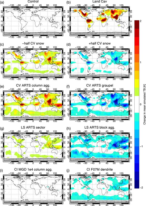
5370                      A. J. Geer: Physical characteristics of frozen hydrometeors inferred with parameter estimation

Da Silva, 2007; Ruckstuhl and Janjić, 2020; Kotsuki et al.,        model moist physics in the parameter estimation, but for the
2020).                                                              moment this is excluded.
   Physical assumptions also need to be made in the for-               The weather forecasting system being used is the Inte-
ward models of satellite radiances that are required for mak-       grated Forecasting System (IFS, ECMWF, 2019) operated by
ing cloud and precipitation retrievals (e.g. Kummerow et al.,       the European Centre for Medium-range Weather Forecasts
2001) or for assimilating such observations in weather fore-        (ECMWF). This is described in Sect. 2.1, and the RTTOV-
casting (e.g. Geer et al., 2018). In particular, all-sky mi-        SCATT observation operator is covered in Sect. 2.2. The ob-
crowave observations are strongly sensitive to macrophys-           servations used in the parameter estimation come from the
ical and microphysical parameters of cloud and precipita-           Special Sensor Microwave Imager/Sounder (SSMIS, Kunkee
tion, most of which are not prognostic variables in forecast        et al., 2008) and are described in Sect. 2.3. The six different
models. For example there is typically only a prognostic de-        microphysical and macrophysical parameters to be optimised
scription of hydrometeor mixing ratio, and if the particle size     are described in Sect. 3. Overall, Sects. 2 and 3 will be seen
distribution (PSD) and particle shape are constrained by as-        to contain a wealth of technical detail, but this is probably
sumed diagnostic relationships in the model, these may not          inescapable in a successful parameter estimation, which still
give good results in the radiative transfer, due to the different   relies on expert knowledge. The method for parameter esti-
physical sensitivities of each context. Further, such assump-       mation is a complete but efficient search of parameter space;
tions are not even necessarily consistent among the differ-         this is described in Sect. 4. Section 5 describes the results of
ent components of one forecast model (Geer et al., 2017a).          global and situation-dependent parameter searches and tests
Hence, setting the physical assumptions used in the radiative       the robustness of the chosen parameter sets. Section 6 is a
transfer consistently with those of the forecast model is rarely    discussion: first, reviewing what has been learnt about phys-
done (e.g. Sieron et al., 2017) and remains a long-term aim.        ical parameters (Sect. 6.1); second, placing this work in the
Instead, as with the development of forecast models, radia-         wider context of parameter estimation studies and Bayesian
tive transfer assumptions have often been set independently         inverse methods (Sect. 6.2). The conclusion is Sect. 7.
and by trial and error, expert knowledge (e.g. Di Michele
et al., 2012), or by closure studies (e.g. Kulie et al., 2010;
Ekelund et al., 2020). Similar to a closure study, a parame-        2     Observations and models
ter search by Geer and Baordo (2014) found a snow particle
                                                                    2.1    Weather forecasting system
shape by minimising the discrepancy between passive mi-
crowave observations and the equivalent radiances simulated
                                                                    The core of this work is to compare model simulations to real
from a forecast model. The current work builds on this by
                                                                    observations, in other words model–observation closure. The
simultaneously estimating the values for six physical param-
                                                                    tools for this are provided within the IFS. The data assimi-
eters relating to frozen hydrometeors and by using a more
                                                                    lation component provides high-quality initial conditions of
sophisticated estimation framework.
                                                                    the earth system (the analysis fields); a short run of the fore-
   This work has dual motivations: one is to explore param-
                                                                    cast model provides the “background” geophysical fields at
eter estimation as a way of using observations to improve
                                                                    the observation time and location, and the observation op-
physical models; another is the more practical issue of updat-
                                                                    erator maps from model fields to the observations – here the
ing the physical assumptions in the RTTOV model (Radia-
                                                                    radiances measured by satellites. The parameter estimation is
tive Transfer for TOVS Saunders et al., 2018) and in partic-
                                                                    done with passive monitoring experiments, which take their
ular its microwave/sub-millimetre scattering radiative trans-
                                                                    background fields from a fixed reference run of the DA sys-
fer component, RTTOV-SCATT (Bauer et al., 2006). Since
                                                                    tem. Hence, the background geophysical fields are (with one
the earlier study (Geer and Baordo, 2014), a wider and more
                                                                    exception) held constant while only the physical assumptions
physical range of frozen particle representations has become
                                                                    in the observation operator are varied.
available (e.g. Kneifel et al., 2018; Eriksson et al., 2018), and
                                                                       Experiments were based around cycle 46r1 of the IFS
the observation operator offers additional PSD choices and
                                                                    (ECMWF, 2019), but adding a development version of RT-
a more flexible representation of hydrometeors (Geer et al.,
                                                                    TOV that is described in the next section. The experiments
2021). There is also a need to prepare for new satellite instru-
                                                                    used a resolution of Tco399 or roughly 28 km horizontally2 .
ments operating at sub-millimetre (sub-mm) wavelengths,
                                                                    There were 137 levels in the vertical, from the surface to
which will be more sensitive to the microphysical properties
                                                                    0.01 hPa. The data assimilation process used to create the
of cloud ice, particularly the Ice Cloud Imager (ICI, Buehler
                                                                    fixed reference analyses used a 12 h cycling 4D-Var (Rabier
et al., 2007; Eriksson et al., 2020). The practical output of
                                                                    et al., 2000) with three inner-loops at TL59/TL255/TL255
this work is therefore to provide the default physical config-
                                                                    resolution3 corresponding to 125 and 78 km respectively. De-
uration for RTTOV-SCATT in v13.0 of RTTOV, which was
released in November 2020 (Saunders et al., 2020). Future              2 T: triangular truncation of the spectral fields; co: cubic octahe-
iterations of this work will also seek to include the forecast      dral reduced Gaussian grid for the gridded fields.
                                                                       3 L: linear reduced Gaussian grid.

Atmos. Meas. Tech., 14, 5369–5395, 2021                                                https://doi.org/10.5194/amt-14-5369-2021
A. J. Geer: Physical characteristics of frozen hydrometeors inferred with parameter estimation                               5371

spite having a slightly lower horizontal resolution compared      ered independent, and hydrometeor optical properties are in-
to the operational version, this still provides high-quality      variant with polarisation. This neglects the polarising effects
background fields and is the standard configuration for test-     of scattering from particles, which can transfer energy from
ing at ECMWF. See Geer et al. (2017b) for a summary of            one polarisation to another, and causes optical properties to
all-sky microwave data usage in the assimilation system and       vary as a function of polarisation and viewing angle. RT-
Hersbach et al. (2020) for a broader overview of data usage       TOV v13.0 will have a simplified treatment of polarised scat-
in the IFS.                                                       tering from preferentially oriented frozen hydrometeors; this
   Cloud and precipitation in the IFS are generated using         reduces errors in the simulated vertical–horizontal polarisa-
a set of physical parametrisations. Large-scale (stratiform)      tion difference by 10–15 K (Barlakas et al., 2021). This is not
cloud and precipitation mixing ratios are prognostic variables    used in the main study; however, the parameter estimation is
that are subject to advection and whose interactions, sources,    updated at the end, taking account of the new polarisation
and sinks are governed by the Tiedtke (1993) parametrisa-         scheme, to provide a self-consistent final configuration for
tion with subsequent improvements (e.g. Tompkins et al.,          RTTOV v13.0 (Sect. 5.4).
2007; Forbes and Tompkins, 2011). Large-scale cloud frac-            The surface interaction is treated as specular reflec-
tion is also a prognostic variable in this scheme. Moist con-     tion. Over ice-free ocean surfaces, this is handled by the
vection is represented by a diagnostic mass-flux parametri-       FASTEM-6 surface emissivity model (Kazumori et al.,
sation (Tiedtke, 1989; Bechtold et al., 2014). The convec-        2016), which includes a simplified treatment for diffuse scat-
tive core hydrometeors are represented by the updraught and       tering. Over sea ice and over land, an all-sky dynamic emis-
downdraught mass fluxes, which are assumed to occupy a            sivity retrieval operates at lower frequencies to supply the
fixed 5 % of the grid box. Cloud water and ice can be de-         surface emissivity for the 50 and 183 GHz sounding chan-
trained into the large-scale scheme, allowing convection to       nels (Baordo and Geer, 2016). The TELSEM surface emis-
form anvil cloud.                                                 sivity database (Aires et al., 2011) is used for the other chan-
                                                                  nels of SSMIS over land surfaces and also as a backup when
2.2   Observation operator                                        the retrieval is not possible. In the passive monitoring exper-
                                                                  iments used here, a change to physical assumptions in the
The observation operator for satellite radiances in the IFS is    radiative transfer can affect the dynamic emissivity retrieval.
RTTOV (Saunders et al., 2018). Within this, RTTOV-SCATT           In practice, the effect is negligible, and even in the convective
(Bauer et al., 2006) provides the all-sky microwave capabil-      graupel experiment (the biggest change tested; see Table 2)
ities. The all-sky radiance simulated by RTTOV-SCATT is           the maximum change in surface emissivity is tiny at around
the weighted combination of radiances from two independent        1e−6 .
column calculations: one that is completely clear, Iclear , and      The scattering solver requires the bulk optical properties
one with horizontally homogeneous cloud and precipitation,        of each layer of atmosphere. Hydrometeor optical proper-
Icloud . The cloudy column is weighted by an effective cloud      ties (extinction, single-scattering albedo, and the asymmetry
fraction C to approximate the nonlinear effect of sub-grid        parameter) are supplied from lookup tables as a function of
variability of cloud and precipitation, which is sometimes        frequency, temperature, hydrometeor type, and hydrometeor
known as the beam-filling effect (e.g. Geer et al., 2009a; Bar-   water content. Changes to the microphysical assumptions ex-
lakas and Eriksson, 2020). Hence the all-sky radiance is          plored in this work were made by changing these lookup ta-
Iall-sky = CIcloud + (1 − C)Iclear .                       (1)    bles, which are generated by an offline tool available within
                                                                  RTTOV (Geer et al., 2021). This integrates single-particle
This is then converted to black-body equivalent brightness        optical properties over the assumed particle size distribution,
temperature (TB, in K), which is the usual, more intuitive        given the water content. It offers a choice of hydrometeor
variable to represent satellite radiance observations. The ef-    representations based on Mie spheres or non-spherical par-
fective cloud fraction C simplifies what could be a complex       ticles from the Liu (2008) and ARTS (Eriksson et al., 2018)
3D arrangement of cloud and precipitation. Two options for        databases. Version 13.0 includes new options for particle size
deriving C will be tested in the parameter search (Sect. 3.1).    distributions that were added in support of the current work.
   In Eq. (1) the clear column accounts only for the surface      From the available options, four sets of parameters relating to
interaction and gaseous absorption. In the cloudy column,         large-scale snow, convective snow, and cloud ice were added
scattering radiative transfer is represented using the delta-     to the parameter estimation as will be described in Sect. 3.
Eddington approach (Joseph et al., 1976; Kummerow, 1993;             As discussed, the IFS has four large-scale prognostic hy-
Bauer et al., 2006). Although simple compared to more exact       drometeors, a prognostic cloud fraction, and a diagnostic
scattering methods, this is fast enough for use in a weather      large-scale precipitation fraction. Additionally, diagnostic
forecasting system and still accurate compared to reference       mass fluxes for snow and rain represent convection, which
models.                                                           is assumed to take 5 % of the grid box area. This is the com-
   One simplification in the scattering radiative transfer is     plete set of cloud and precipitation information provided to
the treatment of polarisation. Each polarisation is consid-       RTTOV-SCATT, although some conversions are needed. To

https://doi.org/10.5194/amt-14-5369-2021                                            Atmos. Meas. Tech., 14, 5369–5395, 2021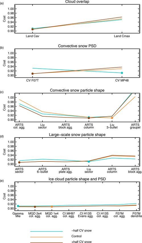
5372                     A. J. Geer: Physical characteristics of frozen hydrometeors inferred with parameter estimation

standardise the treatment with the convection fluxes, all six
hydrometeors (rain, snow, cloud ice, and cloud water from
the large-scale scheme; rain and snow from the convection
scheme) are extracted from the model as fluxes (kg m−2 s−1 )
and then converted to mass mixing ratios (kg kg−1 ) before
input to RTTOV-SCATT (see Geer et al., 2007, Appendix
B). Strictly, this ratio is defined as the mass of the hydrome-
teor with respect the mass of moist air. However, due to the
lack of a widely used terminology to specify whether hy-
drometeor mixing ratios are based on dry or moist air, this       Figure 1. Number of SSMIS F-17 observations (superobs) selected
quantity is referred to throughout as just “mixing ratio”. The    in the 13–22 June 2019 study period per 10◦ by 10◦ latitude–
assumptions involved in obtaining the mixing ratio from the       longitude bin. The colour scale is logarithmic to highlight data-poor
flux make the convective mixing ratio particularly uncertain      areas. White areas have no observations. A total of 916 258 obser-
(Geer et al., 2017a), but rather than adjust the assumptions in   vations are included.
the model, here the parameter estimation is used to estimate
a scaling factor to adjust the convective snow mixing ratio
                                                                  onto an 80 km by 80 km grid (Geer and Bauer, 2010) which
directly – further details in Sect. 3.
                                                                  averages together at least nine original SSMIS observations.
   In the IFS, RTTOV-SCATT has been used in a four-
                                                                  This standardises the resolution across frequencies and helps
hydrometeor configuration until now (rain, snow, cloud wa-
                                                                  match the effective resolution of cloud in the forecast model
ter, cloud ice) with the convective rain and snow mixing ra-
                                                                  (note the simulations are made using the model grid point
tios added together with the large-scale rain and snow re-
                                                                  nearest to the centre of the superob).
spectively; this provides the control setup. Going forward,
                                                                     For the parameter estimation, SSMIS observations are
the aim is a five-hydrometeor configuration, adding a new
                                                                  taken from the F-17 satellite over a 10 d study period from
hydrometeor type specifically for convective snow, which
                                                                  13–22 June 2019 inclusive. The selection of observations
is no longer combined with the large-scale snow. Within
                                                                  aims to include as much data as possible, even in situations
RTTOV-SCATT this hydrometeor is loosely referred to as
                                                                  where the observations are not well-enough represented to be
“graupel”, but strictly it is for convective snow, making no
                                                                  used in active assimilation. The philosophy is that unless dif-
assumptions on the particle habit. The most important causes
                                                                  ficult situations are included as a constraint in the parameter
of uncertainty in the radiative transfer are these microphys-
                                                                  estimation, the quality of radiative transfer in those situations
ical assumptions, along with the representation of sub-grid
                                                                  will never become good enough to allow them to be used.
heterogeneity (Bennartz and Greenwald, 2011; Barlakas and
                                                                  This accepts the risk that unrelated systematic errors, such as
Eriksson, 2020) – hence the attempt to improve these aspects
                                                                  poor surface emissivity, will lead to compensating biases in
through parameter estimation.
                                                                  the parameter estimation.
                                                                     Figure 1 illustrates the number of observations available
2.3    Observations
                                                                  in the study period, using a logarithmic colour scale. These
                                                                  are accumulated in the same 10◦ by 10◦ latitude–longitude
This study uses observations from the Special Sensor Mi-
                                                                  bins that will be used in the cost function for the parameter
crowave Imager/Sounder (SSMIS, Kunkee et al., 2008). This
                                                                  estimation (Sect. 4). Observations are only excluded in areas
is a conical-scanning microwave sensor, meaning that it has
                                                                  of orography higher than 800 m, areas of sea ice, in mixed
an approximately fixed zenith angle and polarisation across
                                                                  scenes where the grid point land–water mask is neither com-
its swath. There are 24 channels on the instrument, of which
                                                                  pletely land or completely ocean, and over land where both
13 have been selected for use in this study (Table 1). Al-
                                                                  the dynamic emissivity retrieval and the atlas backup failed.
though SSMIS has additional calibration issues (e.g. Bell
                                                                  In any one bin, observations must be all ocean or all land,
et al., 2008) compared to later microwave imagers such as the
                                                                  favouring the larger number. Typically around 3000 observa-
GPM microwave imager (GMI, Draper et al., 2015), these are
                                                                  tions are available per bin over ice-free oceans and around
mostly corrected by bias correction, which has been exten-
                                                                  1000 observations over land areas; an approximate total of
sively used at ECMWF for all-sky assimilation and parame-
                                                                  1 million observations is used. The main losses are due to
ter estimation (Geer et al., 2017b; Geer and Baordo, 2014).
                                                                  sea ice, the orography check, and the restriction on mixed
The advantage of using SSMIS is that, with its temperature
                                                                  scenes.
sounding channels around 50 GHz, it is a single instrument
that covers the majority of frequencies currently in use or
planned for use in all-sky assimilation (Geer et al., 2018),      3   Microphysical and macrophysical options
with the main exception being frequencies above 190 GHz,
which will not be available from space until the launch of        This section will outline the six dimensions of the parame-
ICI in 2024. For the IFS, the observations are superobbed         ter search, summarised in Table 2. This is a search among

Atmos. Meas. Tech., 14, 5369–5395, 2021                                             https://doi.org/10.5194/amt-14-5369-2021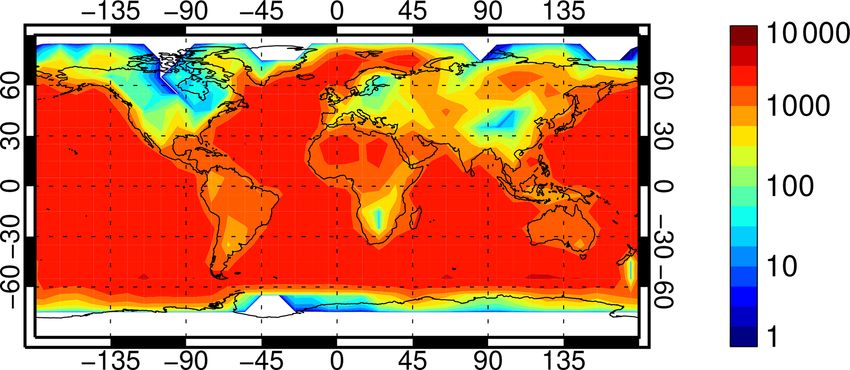
A. J. Geer: Physical characteristics of frozen hydrometeors inferred with parameter estimation 5373
Table 1. SSMIS channels used in this study, ordered by frequency and polarisation.
ID Channel Frequency (GHz) Polarisation Main atmospheric sensitivity
number
19v 13 19.35 v rain
19h 12 19.35 h rain
22v 14 22.235 v TCWV
37v 16 37.0 v TCWV, water cloud, rain
37h 15 37.0 h TCWV, water cloud, rain
50h 1 50.3 h TCWV, water cloud
53h 2 52.8 h LT temperature
92v 17 91.655 v TCWV, water cloud, rain, snow
92h 18 91.655 h TCWV, water cloud, rain, snow
150h 8 150.0 h LT humidity, snow
183 ± 7h 9 183.31 ± 6.6 h MT humidity, snow, ice cloud
183 ± 3h 10 183.31 ± 3.0 h MT humidity, snow, ice cloud
183 ± 1h 11 183.31 ± 1.0 h UT humidity, snow, ice cloud
Pol.: polarisation; v: vertical polarisation; h: horizontal polarisation; TCWV: total column water vapour; LT: lower
troposphere; MT: mid-troposphere; UT: upper troposphere.
discrete possibilities, so the total number of possible config- weighted vertical average of the hydrometeor fractions (Cav ),
urations is the product of the dimension sizes: 2 × 3 × 2 × which is a reasonable approximation to more accurate
6 × 6 × 8 = 3456. Along each dimension, Table 2 orders the multiple-independent column models (Geer et al., 2009a, b);
options according to the all-channel global mean change in this remains fixed in the parameter estimation. But over land
simulated brightness temperature when that parameter is var- surfaces, C has previously been set to the maximum cloud
ied. The main impact of frozen hydrometeors at microwave fraction in the profile, Cmax , not because this is the most
frequencies is to scatter radiation, which generally leads to physically correct approach but to counter systematic errors:
lower brightness temperatures at the top of the atmosphere. Geer and Baordo (2014) took advantage of the fact that Cmax
Hence the dimensions are ordered from the least-scattering generates artificially high scattering TB depressions to com-
options (which increase brightness temperatures compared pensate for the apparent lack of convective cloud and precip-
to the control) to the most scattering (which decrease them). itation over land in the IFS, as seen at frequencies from the
The biggest increase in scattering of any of the options is the microwave to the infrared (e.g. Geer et al., 2019). The hope is
move to a convective graupel particle shape, which reduces that the parameter search can find a configuration that does
brightness temperatures globally by 0.187 K. Such global not require a physically unjustified representation of cloud
mean changes are obviously small, but this is because cloud overlap over land.
and precipitation are localised processes. In heavy precipita- The choice of effective cloud fraction over land affects
tion there are still changes of up to around 100 K, as will be mainly deep convective situations. In the IFS, convective lo-
illustrated later; see also e.g. Geer et al. (2021) for further cations are represented by a convective core occupying 5 %
illustration of the very strong sensitivity of simulated bright- of the model grid box; the anvil is represented by detrainment
ness temperatures to microphysical assumptions. into the large-scale cloud scheme, which typically results in
Although it would be tempting to add more dimensions a thin capping ice cloud with a cloud fraction that is close to
to the parameter search, it soon becomes cumbersome and 1. In the computation of Cav , the convective core typically
would ultimately become impossible due to the curse of di- dominates the mass-weighted average, and hence Cav can
mensionality. The range of options already encompasses re- be as low as 0.05 in convection. By contrast the maximum
search that will take many pages to summarise. More dimen- cloud fraction Cmax is typically found in the anvil cloud and
sions could have been included, particularly in the forecast is typically closer to 1. Hence, using Cmax in Eq. (1) gives
model physics, but that is out of scope of the current study. more weighting to the cloudy column and generates much
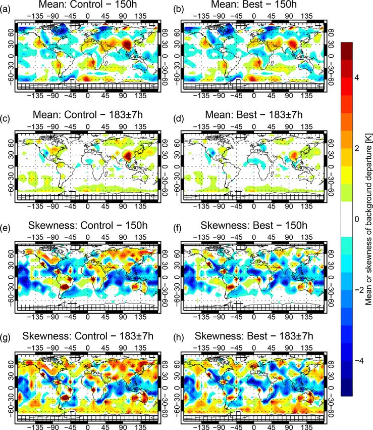
deeper TB depressions. Figure 2b shows that going to Cav in-
3.1 Cloud overlap over land creases the mean simulated brightness temperature in many
land-surface areas. These locations are similar to those af-
As described in Sect. 2.2, sub-grid variability of cloud and fected by increasing convective snow amount (Fig. 2c, d; see
precipitation has a huge effect on the simulated brightness next section), confirming that it is mainly convective situa-
temperatures. This is represented by the effective cloud frac- tions affected.
tion C in the two-column approach used by RTTOV-SCATT
(Eq. 1). Over ocean, C is computed as a hydrometeor-
https://doi.org/10.5194/amt-14-5369-2021 Atmos. Meas. Tech., 14, 5369–5395, 2021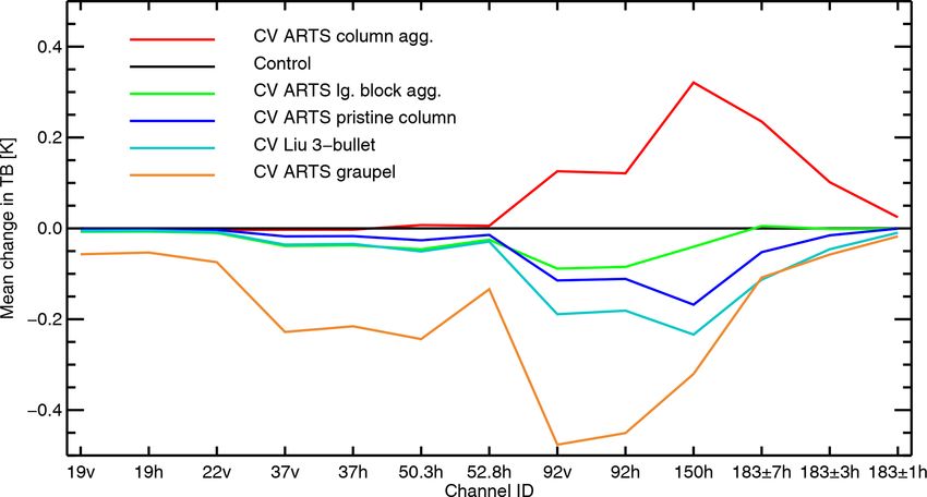
5374                        A. J. Geer: Physical characteristics of frozen hydrometeors inferred with parameter estimation

Table 2. Possible microphysical and macrophysical changes. For details, see text.

         Dimension               Index    Short name                 Description or dimension name                   Mean change
                                                                                                                       in TB (K)
         1. Cloud overlap            1    Land Cav                   Cav effective cloud fraction over land                0.046
                                     2    Control (Land Cmax )       Cmax effective cloud fraction over land                   0
         2. Convective snow          1    −half CV snow              Convective snow mixing ratio scaled by 0.5           0.057
         mixing ratio                2    Control                    Convective snow mixing ratio not scaled                  0
                                     3    +half CV snow              Convective snow mixing ratio scaled by 1.5          −0.046
         3. Convective snow          1    Control (CV F07 T)         Field et al. (2007) tropical PSD for all snow            0
         PSD                         2    CV MP48                    Marshall and Palmer (1948)                          −0.067
         4. Convective snow          1    CV ARTS column agg.        ARTS large column aggregate                          0.071
         particle shape              2    Control (CV Liu sector)    Liu (2008) sector snowflake for all snow                 0
                                     3    CV ARTS block agg.         ARTS large block aggregate                          −0.029
                                     4    CV ARTS column             ARTS column type 1                                  −0.042
                                     5    CV Liu 3-bullet            Liu (2008) 3-bullet rosette                         −0.072
                                     6    CV ARTS graupel            ARTS gem graupel                                    −0.187
         5. Large-scale snow         1    LS ARTS sector             ARTS sector snowflake                                0.054
         particle shape              2    LS ARTS 6-bullet           ARTS 6-bullet rosette                                0.043
                                     3    LS ARTS plate agg.         ARTS large plate aggregate                           0.032
                                     4    Control (LS Liu sector)    Liu (2008) sector snowflake for all snow                 0
                                     5    LS ARTS column             ARTS column type 1                                  −0.065
                                     6    LS ARTS block agg.         ARTS large block aggregate                          −0.090
         6. Ice cloud particle       1    See Table 3
         shape and PSD              ...
                                     8

3.2    Options for convective snow                                      impact on mean brightness temperatures and reveal the loca-
                                                                        tions where significant convection occurred during the 10 d
                                                                        study period: around the ITCZ, in the SH storm tracks, and at
The physical parameters of convective snow are not well                 midlatitudes over land surfaces. Adding the convective mix-
known and may explain many of the largest errors in the ob-             ing ratio as a parameter is not intended to provide a scaling
servation operator. In addition, the model-derived convective           factor to be included in a future observation operator but in-
snow mixing ratio is quite uncertain. One source of uncer-              stead to explore the robustness of the results to one of the
tainty already mentioned (Sect. 2.2) is the conversion from             biggest uncertainties and to point to areas needing future im-
convective mass flux to mixing ratio, which makes assump-               provement.
tions on the PSD and the fall-speed distribution. The assumed              Turning to the other convection-related parameters, large
fall speeds are suspected of being too low for convective               hail particles are important in the generation of extreme
particles (Geer et al., 2017a, Sect. 3.3). This could lead to           brightness temperature depressions (e.g. Zipser et al., 2006).
convective snow mixing ratios being overestimated by about              Intense convection can generate hail in excess of 127 mm in
50 %. However, as discussed in the previous subsection, the             size (Allen et al., 2017); direct observations from within se-
observational evidence from all-sky infrared assimilation is            vere convection are difficult, but an armoured research air-
consistent with the convective mixing ratio being too low,              craft has been able to sample PSDs of hail up to 50 mm in
particularly over land (Geer et al., 2019). This could come             size (Field et al., 2019). Hence, dimension 3 of the parameter
from known deficiencies in the convection scheme, such as               search (Table 2) explores the convective snow PSD. The con-
insufficient convection at night over land (Bechtold et al.,            trol uses the Field et al. (2007, F07) tropical (T) PSD for all
2014). To simplify the current parameter estimation, it was             frozen precipitation. However, this was derived from in situ
not attempted to address these uncertainties at their physical          measurements of tropical anvils and midlatitude stratiform
source but to treat the convective mixing ratio as an uncertain         clouds, so it may not be appropriate for the large frozen par-
parameter. Dimension 2 of the parameter search (Table 2)                ticles within the convective cores. The Marshall and Palmer
allows the model-derived convective snow mixing ratio to                (1948) PSD is provided as an alternative in the parameter
be increased or decreased by 50 %. This scaling is applied              search; as implemented here this boosts the number of large
across the whole vertical profile. Figure 2c and d show the

Atmos. Meas. Tech., 14, 5369–5395, 2021                                                    https://doi.org/10.5194/amt-14-5369-2021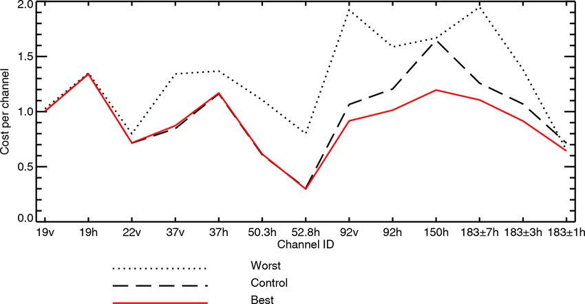
A. J. Geer: Physical characteristics of frozen hydrometeors inferred with parameter estimation                                       5375

Figure 2. Mean change in simulated brightness temperatures when using some of the options from Table 2, compared to the control. Statistics
are based on a 10 d period and shown for SSMIS channel 150h, which is generally the channel with the largest impact from changes in the
physical assumptions for frozen hydrometeors.

particles (≥ 10 mm) by at least 2 orders of magnitude com-                 Another potential adjustment for convective snow is the
pared to the F07 PSD and hence gives more scattering (see               particle shape. Note that the particle shape also implies a
Geer et al., 2021, for more details). The effects of this are           mass–size relation, and hence this affects the bulk scatter-
not illustrated as they are broadly similar to increasing the           ing properties through adjustments to both the size distribu-
convective snow mixing ratio by 50 %.                                   tion and the single-scattering characteristics (Eriksson et al.,
                                                                        2015; Geer et al., 2021). The Liu (2008) sector snowflake is

https://doi.org/10.5194/amt-14-5369-2021                                                   Atmos. Meas. Tech., 14, 5369–5395, 2021
5376 A. J. Geer: Physical characteristics of frozen hydrometeors inferred with parameter estimation
used in the control, since this was the best particle to repre- ARTS block aggregate generate more scattering and lead to
sent the sum of convective and large-scale snow in the pa- colder brightness temperatures.
rameter search of Geer and Baordo (2014). However it is an Figure 2g and h show the geographical effect of changing
idealised smooth and solid particle that will be inadequate the large-scale snow particle shape. This highlights areas of
to represent scattering in future sub-mm applications (Fox significant large-scale precipitation during the 10 d study pe-
et al., 2019). The ARTS database offers new options of ice riod, including the SH storm tracks, the western Pacific and
aggregates and graupel, and these may be more physically the Atlantic coast of North America. Although there is some
representative (Eriksson et al., 2018). Hence in the fourth overlap with the spatial pattern of convection seen in Fig. 2c
dimension of the search, particle types have been chosen and d, there are also distinct differences – for example in
to sample different levels of scattering and also some very North America, convection dominates over the midwest and
different physical representations: the ARTS column aggre- large-scale precipitation over the Atlantic coast. This sug-
gate4 generates less scattering than the Liu sector, whereas gests that the convective and large-scale physical parameters
the ARTS block aggregate, column, and gem graupel gen- should be independently identifiable through their spatial sig-
erate increasingly more scattering. The options also include natures. And as with the convective snow particle choices,
the Liu (2008) 3-bullet rosette, which was found by Geer and there is also spectral differentiation between the large-scale
Baordo (2014) to give the best results when convective snow snow shapes that should further improve identifiability (see
was represented separately to large-scale snow. It is striking Geer et al., 2021).
that the particle shape assumptions illustrated in Fig. 2e and f
have a larger impact on the simulated TB than a 50 % change 3.4 Options for cloud ice
in the mass mixing ratio (as seen in Fig. 2c and d).
Figure 3 illustrates the frequency-resolved global mean The current representation of ice cloud in RTTOV-SCATT
change in brightness temperature coming from changes in uses a Mie sphere combined with a gamma PSD and is phys-
convective particle shape. Graupel generates significantly in- ically unrealistic (Geer and Baordo, 2014). Ice cloud is ex-
creased scattering down to 19 GHz and has its biggest effect pected to have a small effect on radiances at 183 GHz (e.g.
around 92 GHz. The other chosen particles do not change the Hong et al., 2005; Doherty et al., 2007), but in the control
results so much at frequencies below 92 GHz, but there is configuration it has almost no effect (not shown). However
plenty of variability in the higher frequencies. For example, there is sensitivity at 183 GHz and below (Geer et al., 2021),
the ARTS column and ARTS block aggregate would reduce so it is hoped to find a baseline representation of ice cloud
TBs by similar amounts at 92 GHz, but they have different that can be further improved once ICI has been launched.
effects at 150 GHz. Hence there is a spectral signature asso- Table 3 summarises the ice cloud options in the param-
ciated with the snow particle shape that should help resolve eter search, and further details can be found in Geer et al.
any ambiguity with changes in mixing ratio. For further il- (2021). The highest-scattering option is the combination of
lustration of the spectral signatures of these particles, see the Field et al. (2007) PSD and Liu (2008) dendrite, simi-
Geer et al. (2021); in heavy cloud situations these choices lar to the configuration which gave the best results for ice
can change the simulated brightness temperature by up to cloud in the fine search of Geer and Baordo (2014) but us-
150 K. ing the F07 PSD midlatitude option (M), rather than tropi-
cal option, to reduce the number of large particles. Figure 2j
3.3 Options for large-scale snow shows this configuration decreases brightness temperatures
in many areas compared to the control. However, preliminary
The representation of large-scale snow is not perfect but experimentation suggested there was too much scattering in
probably better than that of convection. Hence only a sin- this configuration. It is only with the new particle shapes and
gle dimension is explored – that of particle shape, as shown PSDs in RTTOV-SCATT that lower-scattering options have
in Table 2. The Field et al. (2007) tropical PSD was retained become available (Geer et al., 2021). From the ARTS parti-
for large-scale snow in all experiments, mainly to reduce the cle database, the ARTS column aggregate and the Evans ag-
search space, but also because this PSD is well established in gregate generate less scattering. Also a range of alternative
this context (e.g. Fox et al., 2019). Among the particle shape PSDs help reduce the number of large particles and hence
options, the ARTS sector snowflake is a separate option to reduce the overall amount of scattering. As shown in the ta-
the Liu sector snowflake from the control, and it generates ble, progressively less scattering can be generated using the
warmer mean brightness temperatures (see Geer et al., 2021; McFarquhar and Heymsfield (1997, MH97) and Heymsfield
this is due to differing mass–size relations; the single-particle et al. (2013, H2013) PSDs. Early attempts at the parame-
optical properties are near identical). The ARTS column and ter search suggested that even less-scattering options might
be required, so two ad hoc PSDs were created using the
4 The ARTS aggregates here are based on the “large” pris- all-purpose modified gamma distribution (MGD; Petty and
tine particles, but since there are no “small” versions available in Huang, 2011); these are known as the MGD 2e4 and MGD
RTTOV-SCATT, the distinction is not always made. 1e4 PSDs, with the number referring to the lambda parame-
Atmos. Meas. Tech., 14, 5369–5395, 2021 https://doi.org/10.5194/amt-14-5369-2021A. J. Geer: Physical characteristics of frozen hydrometeors inferred with parameter estimation 5377
Figure 3. Global mean change in simulated brightness temperature when using different options for the shape of convective snow, compared
to the control in which the Liu sector snowflake is used for all snow.
Table 3. Possible microphysical changes for cloud ice.
Index Short name Particle shape PSD Mean change
in TB (K)
1 Control (gamma Mie) Mie sphere with ρ = 900 kg m−1 MGD with µ = 2, 3 = 2.05 ×10⁵ m−1 , γ = 1 0
2 CI MGD 2e4 ARTS large column aggregate MGD with µ = 0, 3 = 2.0 × 10⁴ m−1 , γ = 1 −0.004
3 CI MGD 1e4 ARTS large column aggregate MGD with µ = 0, 3 = 1.0 × 10⁴ m−1 , γ = 1 −0.019
4 CI MH97 ARTS large column aggregate McFarquhar and Heymsfield (1997) −0.030
5 CI H13 Evans ARTS Evans aggregate Heymsfield et al. (2013) stratiform −0.032
6 CI H13 col. agg. ARTS large column aggregate Heymsfield et al. (2013) stratiform −0.035
7 CI F07 M col. agg. ARTS large column aggregate Field et al. (2007) midlatitude −0.044
8 CI F07 M dendrite Liu (2008) dendrite Field et al. (2007) midlatitude −0.070
ter in the MGD. The configurations using these PSDs make justified a posteriori. This meant that only one experiment
only small changes compared to the control (e.g. Fig. 2i). needed to be run for each of the parameter options described
Figure 2j shows that ice cloud effects can be seen in con- in Sect. 3, in addition to the control – a total of 22 exper-
vective and large-scale areas alike, so ice cloud has its own iments. An alternative to running the full IFS would have
distinct spatial signature; there are also some frequency sig- been to archive the necessary geophysical inputs to RTTOV-
natures (such as differences between the MH97 and H2013 SCATT for around 106 observations, but significant storage
options, thought to be due to different temperature depen- and computation resources would still have been needed.
dences in the PSDs, not shown). Hence there is hope that ice The assumption of linearly additive perturbations is ex-
cloud parameters will be identifiable in this work. pressed mathematically as
X
Ti,j,v ' Tcontrol + Ti,j,vk − Tcontrol . (2)
k
4 Parameter estimation method
Here, T is the simulated brightness temperature, i the index
4.1 Search across the approximately 106 observations, and j the index
across the 13 selected channels of SSMIS. k is the index
There are 3456 different parameter combinations available, across six search dimensions and vk the index within each
and it was not feasible to evaluate every combination directly, search dimension. v is a vector containing the six vk indices.
since each would require a passive monitoring run of the Tcontrol is the brightness temperature simulated in the control
IFS. Instead the cost function was evaluated approximately experiment. As an example, the “intermediate” configuration
at each point in the search space. This was done using an from Sect. 5.4 is
assumption of linearly additive perturbations, which will be
https://doi.org/10.5194/amt-14-5369-2021 Atmos. Meas. Tech., 14, 5369–5395, 20215378 A. J. Geer: Physical characteristics of frozen hydrometeors inferred with parameter estimation
1 Land Cav
2
Control
1 Control
v intermediate = = . (3)
5
CV Liu 3-bullet
1 LS ARTS sector
6 CI H13 col. agg.
In the parameter search, the effect of these choices on
the brightness temperature was estimated as follows, using
Eq. (2):
Tv intermediate ' TLand Cav + TCI H13 + TLS ARTS sector
+ TCV Liu 3-bullet − 3 × TControl . (4)
Note that for simplicity the i and j indices have been dropped
here. Figure 4. Scatter plot of change in channel 92v brightness temper-
Figure 4 illustrates the validity of the linear assumption for ature, relative to control, when going to the “intermediate” physical
the intermediate configuration. This is a scatter plot based on configuration from Sect. 5.4 (Land Cav , CV Liu 3-bullet, LS ARTS
the left and right sides of Eq. (4) after subtracting TControl . sector, CI H13). On the y axis this is estimated using the assump-
The estimate falls around 30 % below the 1 : 1 line for the tion of linearly additive perturbations, by subtracting TControl from
largest perturbations (≥ 10 K); these points are located in Eq. (4). On the x axis the intermediate configuration has been eval-
uated by running an experiment with exactly that configuration.
convective land areas (not shown), suggesting that the two
convection-related changes (Land Cav and CV Liu 3-bullet)
do not combine linearly, which can hardly be expected. How-
of the departure normalised by the observation error, follow-
ever, the estimate has errors mostly less than 2 K for smaller
ing an assumption of Gaussian errors (see e.g. Geer, 2021).
perturbations. The standard deviation of the difference be-
The best fit to observations, known as the analysis, is ob-
tween the estimated and actual perturbation is 0.96 K, sug-
tained where the cost function has a minimum.
gesting that the assumption is valid to reasonable accuracy in
The square of the departure is a poor choice of cost met-
most situations. On maps, the linear-estimated and nonlinear-
ric when it comes to cloud and precipitation. One reason
computed results are surprisingly difficult to tell apart by eye
is that modelled and observed clouds are not always in the
(not shown; this applies both to the brightness temperatures
same place, so it is often possible to reduce the squared
and the binned statistics like those used in the cost function,
error by removing the simulated cloud or precipitation –
Sect. 4.2). Similar levels of accuracy have been seen with
this is known as the double-penalty effect. As explored by
other configurations. However, for the same reason the as-
Geer and Baordo (2014), more appropriate cost functions
sumption is needed in the first place, it is hard to test it ex-
for cloud and precipitation parameter estimation could in-
haustively; possible future improvements are discussed in the
clude the mean and skewness of departures, or measures of
conclusion.
fit between the observed and simulated probability distribu-
4.2 Cost function tion function (PDF) of brightness temperatures, using mea-
sures similar to the Kullback–Leibler divergence (Kullback
In order to choose a unique “best” configuration, there must and Leibler, 1951). The PDF divergence approach was not
be a single objective way to measure the fit between the pursued here because it is hard to combine with geographi-
model and the observations. Following the data assimilation cal binning (see below) which is used to help make the pa-
approach, this is provided by a cost function based on the de- rameters more identifiable. A vastly larger dataset would be
parture d between the observation and the simulated equiva- needed to ensure good sampling of the brightness tempera-
lent: ture PDFs in each geographical bin.
In order to have a single cost function to minimise, a com-
observed simulated bination of the mean and skewness of the departures was cho-
di,j,v = Ti,j − bi,j − Ti,j,v . (5)
sen for the current parameter estimation. Section 5.2 explores
Here bi,j is an observation bias correction estimated using alternative choices. The mean and skewness are computed in
variational bias correction (VarBC, Dee, 2004; Auligné et al., 10◦ by 10◦ latitude–longitude bins (Fig. 1). Then the abso-
2007) within the weather forecasting framework, which will lute value in each geographical bin is combined, giving the
be discussed shortly. In a data assimilation cost function, the following cost function:
equivalent “observation term” is usually based on the square
Atmos. Meas. Tech., 14, 5369–5395, 2021 https://doi.org/10.5194/amt-14-5369-2021A. J. Geer: Physical characteristics of frozen hydrometeors inferred with parameter estimation 5379
the total column water vapour (TCWV), skin temperature,
and surface wind speed. For sounding channels, they include
1X 1X functions of the layer thickness (an average temperature, es-
J (v) = 0.5 Mean Binl di,j,v
m j n l sentially). None of the predictors is directly correlated with
! cloud-related biases, so these do not map directly onto the
1X VarBC bias correction. In some channels the bias correction
+0.5 Skew Binl di,j,v . (6)
n l aliases some of the latitude-dependent biases, such as dif-
ferences between tropical and midlatitude cloud simulations,
Here l is an index over all n geographical bins that con- but the effect is generally small. Ideally VarBC would be al-
tain data (bins with 10 or fewer observations are ignored), lowed to vary, but as a first approximation it is held constant.
|·| computes the absolute value, Binl (·) represents the geo-
graphical subset of observations in bin l, Mean(·) computes
the mean of a set of departures, and Skew(·) computes the 5 Results
skewness (with zero being a perfectly symmetric PDF of de-
partures). The inner sum is over geographical bins, and the 5.1 Global parameter search
outer sum is over the m selected SSMIS channels j . The aim
of the parameter search is to find the set of physical choices The first application of the parameter search is to find a sin-
v that minimises the cost function J (v). gle set of physical parameters that would provide the best fit
The form of cost function in Eq. (6) has a number of ad- globally, a one-shape-fits-all approach. Figure 5 helps to vi-
vantages. A single global mean is of little use, since it allows sualise the six-dimensional cost function by showing slices
different situation-dependent biases to be summed together. along its dimensions at the control configuration and at the
A set of physical choices leading to compensating system- best configuration. At the control configuration, perturba-
atic errors could score as well as a set with smaller system- tions in most directions would increase cost: for example, all
atic error. As illustrated in Fig. 7, geographical separation other choices of convective snow particle would make things
helps to implement an approximate regime-based separation worse. This indicates that the configuration provided by Geer
– for example the errors over tropical land surfaces are sepa- and Baordo (2014) was already at a reasonably stable local
rated from those in frontal cloud in the storm tracks and can- minimum.
not compensate for each other. It is also helpful to compute The best configuration is summarised in Table 4. Here,
the skewness in geographical bins, as this measure can oth- the shape of the cost function is very different (Fig. 5). The
erwise be dominated by the large departures in the vicinity largest difference is the reversal in the gradient of the cost
of tropical convection. As will be seen later, this is a signif- function with respect to cloud overlap. Cav overlap over land
icant advance on the use of a global skewness by Geer and is now clearly better than the Cmax overlap used in the con-
Baordo (2014) because it helps identify problems with the trol. Another big difference is that the choice of convec-
use of Cmax over higher-latitude land surfaces, an issue that tive snow particle is now well bounded at the extremes: at
was missed in the earlier work. low-scattering the ARTS column aggregate has high cost
Unlike a typical data assimilation cost function, the er- and is clearly inappropriate; at the high-scattering end the
ror in the observations is not considered in Eq. (6). It is as- ARTS graupel also gives a high cost. The ARTS column is
sumed that given the large numbers of observations in most marginally the best, but the ARTS block aggregate or Liu
bins (Fig. 1), the mean or skewness of the binned sample is 3-bullet would be a reasonable alternative. A final big differ-
mostly insensitive to observation error. Normal data assimi- ence is the change in the gradient of the cost function with
lation also includes a background term measuring the devia- respect to convective snow mixing ratio. At the best configu-
tion from prior knowledge, and also serving to regularise the ration, the mixing ratio should be increased by 50 %, whereas
problem. Section 6.2 discusses the issue of prior knowledge the control configuration could have been improved by re-
further, and regularisation is not needed as the problem is ducing the mixing ratio by the same amount.
likely to be well determined, with six unknowns and around There are smaller changes in the other dimensions in
106 observations. Fig. 5. For the large-scale snow, a small improvement is
The VarBC bias correction, bi,j in Eq. (5), is fixed found going to the ARTS sector, although the ARTS 6-bullet,
throughout the passive monitoring experiments conducted ARTS plate aggregate, or Liu sector (the control configu-
here. A large part of the modelled bias, especially for SS- ration) would produce similar results. The lower-scattering
MIS, is thought to come from the instrument calibration, end is not bounded, so it might be possible to further im-
so it is necessary to include a bias correction. VarBC esti- prove the simulations with a less-scattering configuration for
mates the bias as a linear combination of a globally constant large-scale snow. The least constrained dimension is the ice
offset, a number of polynomial terms based on the instru- cloud microphysics: all configurations produce similar cost,
ment’s scan angle, and a number of model-based predictors. with the MGD 1e4 PSD being only marginally better than
For surface-sensitive observations over ocean, these include the others. Only the F07M PSD with the Liu dendrite shows
https://doi.org/10.5194/amt-14-5369-2021 Atmos. Meas. Tech., 14, 5369–5395, 20215380 A. J. Geer: Physical characteristics of frozen hydrometeors inferred with parameter estimation Figure 5. Slices through the six-dimensional cost function around the control configuration (dashed) and around the best configuration (solid; see also Table 4). The dimensions are ordered from least-scattering to most-scattering options. The dots indicate the parameter settings for the control and for the very best (lowest cost) configuration. Atmos. Meas. Tech., 14, 5369–5395, 2021 https://doi.org/10.5194/amt-14-5369-2021
A. J. Geer: Physical characteristics of frozen hydrometeors inferred with parameter estimation                               5381

Table 4. Results of parameter search.                              ative skewness in the ITCZ over central Africa at 150 GHz
                                                                   and 183 ± 3 GHz and slightly more positive skewness over
      Dimension/metric                   Best                      the Southern Ocean at 183 GHz. To better understand these
      Cloud overlap                      Land Cav
                                                                   changes, Fig. 8 shows the histograms of brightness tempera-
      Convective snow mixing ratio       +half CV snow             tures at 150 GHz over land, separated into broadly extratrop-
      Convective snow PSD                Control                   ical and tropical areas using a TCWV threshold. In extratrop-
      Convective snow particle shape     CV ARTS column            ical locations the control has an order of magnitude too many
      Large-scale snow particle shape    LS ARTS sector            occurrences of strong scattering (TBs less than 210 K) com-
      Ice cloud particle shape and PSD   CI gamma 2e4              pared to observations, and the “best” configuration provides
      Cost function (control = 0.925)    0.908
                                                                   a much better distribution. This change is consistent with the
                                                                   move from positive to neutral skewness in extratropical land
                                                                   areas in Fig. 7. It is mainly the result of changing from Cmax
                                                                   to hydrometeor-weighted Cav cloud overlap over land sur-
a visibly increased cost; as previously mentioned this was         faces.
identified in initial work as having too much scattering. Ta-         In contrast to the improvements over extratropical land
ble 4 summarises the best global configuration: overall this       surfaces, Fig. 8b shows that in tropical areas an overestimate
reduces cost to 0.908, compared to 0.925 at the control. This      of strong scattering events has been replaced by a more se-
is only a small improvement, despite major adjustments to          vere underestimation, consistent with the move to negative
the parameters. As will be seen, these adjustments bring a         skewness in tropical convective areas. This exposes the prob-
mix of improvements and degradations that is overall just          lem of missing convection that the Cmax overlap had previ-
slightly better according to the cost function. Section 5.2 will   ously helped to hide. The best configuration (Table 4) also
show that bigger improvements can only come about by mak-          includes an increased convective mixing ratio and the move
ing the parameters situation-dependent.                            to ARTS column to represent convective snow, both of which
   Figure 6 examines the cost function broken down by SS-          significantly increase scattering (Table 2, Fig. 7); however,
MIS channel. The best option improves the fit to observa-          this is not enough to fully compensate. This worsening of re-
tions (reduced cost compared to control) in channels from          sults over tropical land surfaces illustrates the trade-offs re-
92v to 183 ± 1h. This can be contrasted with the worst pos-        quired by a global parameter estimation and helps explain
sible option in the parameter search (the dotted line) which       why the overall cost has not decreased by much.
makes the cost higher in channels down to 22v. The worst              Figure 9 illustrates the changes to the simulated SSMIS
possible option chooses all the most-scattering options avail-     150h brightness temperatures over Africa, Europe, and the
able, such as the ARTS gem graupel particle for convective         Atlantic, on a day with a broad variety of cloud and precip-
snow, and generates significantly increased scattering at low      itation features across these areas. Brightness temperatures
frequencies (20 to 50 GHz; see also Fig. 3), which does not        below 240 K over land surfaces typically indicate scattering
agree with observations; this was also one of the problems         from convective snow. Simulated brightness temperatures in
with the Mie sphere snow representation rejected by Geer           panels (c) and (d) are similar to the observations in panel (b),
and Baordo (2014). The high-scattering options, including          but with the exact placement of convection often in different
the ARTS graupel and the Mie sphere, tend to put deep TB           locations – hence the need for a cost function that is resis-
depressions everywhere there is convection. But in the ob-         tant to the double-penalty effect. Over land, simulated TBs
servations, deep scattering TB depressions are seen at these       have increased by up to 100 K (panel a, where the changes
frequencies only in the very most intense convection (e.g.         are off scale), corresponding to the changes in the TB his-
Zipser et al., 2006). The new search continues to constrain        tograms discussed in previous paragraphs. Over the ocean,
the choices to those that have relatively low scattering at the    there is a general slight decrease in brightness temperatures
lower frequencies, while still being able to produce signifi-      and hence an increase in scattering. Here, the cloud overlap
cant scattering at higher frequencies. This illustrates the im-    is not changed, but the other four changes in the best config-
portance of including the lower frequencies in the cost func-      uration (Table 4) decrease brightness temperatures by up to
tion.                                                              5 to 10 K in cloud and precipitation areas, such as convec-
   Figure 7 shows maps of the mean and skewness of depar-          tion in the ITCZ around 8◦ N, and in an extratropical cyclone
tures in the geographical bins that make up the cost function      in the North Atlantic. These changes are also present in the
(Eq. 6). The best option improves the mean of binned de-           southern extratropics and are likely responsible for the re-
partures over extratropical land surfaces, particularly in the     duction in mean departures over the Southern Ocean in the
NH at 183 ± 3 GHz. The skewness of binned departures in            183 ± 7 GHz channel (Fig. 7c and d).
the control is around +3 in many of these areas; the best
option reduces skewness mostly to the range −1 to +1, at
both 150 GHz and 183 ± 3 GHz. However, some areas show
worse levels of skewness. For example, there is more neg-

https://doi.org/10.5194/amt-14-5369-2021                                             Atmos. Meas. Tech., 14, 5369–5395, 2021
You can also read