The importance of antecedent vegetation and drought conditions as global drivers of burnt area
←
→
Page content transcription
If your browser does not render page correctly, please read the page content below
Biogeosciences, 18, 3861–3879, 2021
https://doi.org/10.5194/bg-18-3861-2021
© Author(s) 2021. This work is distributed under
the Creative Commons Attribution 4.0 License.

The importance of antecedent vegetation and drought conditions
as global drivers of burnt area
Alexander Kuhn-Régnier1,2 , Apostolos Voulgarakis1,2,3 , Peer Nowack2,4,5 , Matthias Forkel6 , I. Colin Prentice1,7 , and
Sandy P. Harrison1,8
1 Leverhulme  Centre for Wildfires, Environment, and Society, London, SW7 2AZ, UK
2 Department  of Physics, Imperial College London, London, SW7 2AZ, UK
3 School of Environmental Engineering, Technical University of Crete, Chania, Kounoupidiana,

Akrotiri, 73100 Chania, Greece
4 Grantham Institute and the Data Science Institute, Imperial College London, London, SW7 2AZ, UK
5 Climatic Research Unit, School of Environmental Sciences, University of East Anglia, Norwich, NR4 7TJ, UK
6 Environmental Remote Sensing Group, TU Dresden, Dresden, Germany
7 Department of Life Sciences, Imperial College London, London, SW7 2AZ, UK
8 Geography and Environmental Science, University of Reading, Reading, RG6 6AB, UK

Correspondence: Alexander Kuhn-Régnier (alexander.kuhn-regnier14@imperial.ac.uk)

Received: 5 November 2020 – Discussion started: 11 November 2020
Revised: 6 May 2021 – Accepted: 18 May 2021 – Published: 29 June 2021

Abstract. The seasonal and longer-term dynamics of fuel ac-     ing. The length of the period which needs to be considered
cumulation affect fire seasonality and the occurrence of ex-    varies across biomes; fuel-limited regions are sensitive to an-
treme wildfires. Failure to account for their influence may     tecedent conditions that determine fuel build-up over longer
help to explain why state-of-the-art fire models do not sim-    time periods (∼ 4 months), while moisture-limited regions
ulate the length and timing of the fire season or interan-      are more sensitive to current conditions that regulate fuel dry-
nual variability in burnt area well. We investigated the im-    ing.
pact of accounting for different timescales of fuel produc-
tion and accumulation on burnt area using a suite of ran-
dom forest regression models that included the immediate
impact of climate, vegetation, and human influences in a        1   Introduction
given month and tested the impact of various combinations
of antecedent conditions in four productivity-related vege-     Wildfires are an important natural disturbance of the Earth
tation indices and in antecedent moisture conditions. Anal-     system. They have extensive socio-economic impacts as well
yses were conducted for the period from 2010 to 2015 in-        as profound effects on vegetation, atmospheric composi-
clusive. Inclusion of antecedent vegetation conditions rep-     tion, and climate (Bowman et al., 2011; Voulgarakis and
resenting fuel build-up led to an improvement of the global,    Field, 2015; Andela et al., 2017; Lasslop et al., 2019). How
climatological out-of-sample R 2 from 0.579 to 0.701, but the   fire regimes may change in the future and how fire-related
inclusion of antecedent vegetation conditions on timescales     feedbacks may influence climate and global environmental
≥ 1 year had no impact on simulated burnt area. Current         changes are growing concerns.
moisture levels were the dominant influence on fuel dry-           The factors that influence the occurrence and intensity of
ing. Additionally, antecedent moisture levels were important    fire are well known: the presence of an ignition source, veg-
for fuel build-up. The models also enabled the visualisation    etation properties that determine the availability of fuel, and
of interactions between variables, such as the importance       weather conditions that promote fuel drying and thereby the
of antecedent productivity coupled with instantaneous dry-      rate of fire spread. However, these factors are strongly cou-
                                                                pled to one another. Climate conditions influence the inci-

Published by Copernicus Publications on behalf of the European Geosciences Union.
3862                                                A. Kuhn-Régnier et al.: Importance of fuel-related vegetation properties

dence of lightning and the nature of the vegetation, while          et al. (2019a) and Hantson et al. (2020) argued for a bet-
wind strength and the impact of atmospheric conditions on           ter understanding of how vegetation properties control fuel
drying are modulated by vegetation cover. Furthermore, the          build-up and therefore fire occurrence and intensity.
relationships among ignitions, vegetation, and climate may             Fuel is organic matter that is available for ignition (Keane
depend on the timescales involved; short-term drought pro-          et al., 2001). The type, amount, and spatial arrangement of
motes fuel drying and hence increases fire risk, but in the         fuel affect its tendency to burn (Archibald et al., 2009). These
longer term, drought conditions reduce vegetation cover and         properties, dictated by vegetation, in turn affect fuel connec-
fuel loads. This complexity makes it challenging to disentan-       tivity and hence fire spread in addition to how rapidly fuel
gle the causes of observed changes in fire activity.                dries out and becomes combustible. Antecedent weather con-
   Furthermore, recent declines in burnt area (BA) in some          ditions in the weeks to years before fire events can determine
regions have been explained as a consequence of human               fuel availability (van Oldenborgh et al., 2021) and hence fire
activity, through indirect and direct intervention (Martínez        occurrence. The effect of antecedent weather conditions on
et al., 2009; Andela et al., 2017), albeit modulated by cli-        BA may depend on the types of vegetation present (which
mate and vegetation (Forkel et al., 2019b). Such human in-          influences whether fuel drying or accumulation is most im-
tervention can promote or suppress fire through ignitions,          portant): antecedent precipitation will increase BA in fuel-
fuel management, and landscape modification. A mainly-              limited regions, for example, but decrease BA in regions
temperature-driven increase in conditions conducive to wild-        where fuel drying is the major control (Alvarado et al., 2020;
fires was suggested by a number of regional studies (e.g.           Abatzoglou and Kolden, 2013; Littell et al., 2009).
Westerling, 2006; van Oldenborgh et al., 2021; Goss et al.,            A number of regional and global studies have indicated the
2020; Barbero et al., 2015). At the global scale, Abatzoglou        importance of antecedent fuel build-up for BA. For exam-
et al. (2019) showed that anthropogenic climate change had          ple, links between fire activity and antecedent productivity
led to an increase in fire weather over 22 % of the global          have been found in South Africa (Van Wilgen et al., 2000),
burnable area by 2019, while Jolly et al. (2015) found that         central Australia (Griffin et al., 1983), grass and shrublands
anthropogenic climate change has led to a lengthening of            in the western United States (Littell et al., 2009; Westerling
the fire season across more than a quarter of global vege-          et al., 2003; Swetnam and Betancourt, 1998), New South
tated land in recent decades. Increases in fire weather are         Wales, Australia, for bushfire fuel (Jenkins et al., 2020), and
predicted under different assumptions about levels of future        southern Africa (Archibald et al., 2009). Global studies have
warming (e.g. Burton et al., 2018; Turco et al., 2018; Bedia        identified similar relationships (a positive relationship be-
et al., 2015).                                                      tween pre-season productivity and fire activity in the follow-
   Understanding the interplay among the different present-         ing dry season) in some dry areas. By studying the correla-
day controls of fire is also a key requirement for the predic-      tion between growing period (i.e. antecedent) soil moisture
tion of future fire-regime shifts and impacts on the land bio-      and fire activity, Krawchuk and Moritz (2011) found fire ac-
sphere and human activities. Coupled fire–vegetation models         tivity in dry regions to be related to antecedent productivity.
can be used to predict changes in large-scale fire regimes in       Similarly, van der Werf et al. (2008) found a similar rela-
response to future climate change scenarios (see e.g. Knorr         tionship for arid ecosystem (e.g. northern Australia), where
et al., 2016; Kloster et al., 2012) and to explore how these        antecedent wet conditions coupled with instantaneous dry-
changes are affected by and will affect regional vegetation         ing were found to be important. Other global studies have
patterns and climate. Although these models are reasonably          also identified northern Australia as obeying this relation-
good at simulating modern geographical fire patterns in BA,         ship (Randerson et al., 2005; Spessa et al., 2005). In a more
they are poor at reproducing observed fire-season length            recent global analysis, O et al. (2020) found that for arid re-
and inter-annual variability (IAV) in BA (Hantson et al.,           gions, wet anomalies (soil moisture) led to increased fire later
2020). Furthermore, there are large differences in their pre-       in the year by increasing fuel loads and biomass. Thus, it is
dictions of both historical (Teckentrup et al., 2019) and fu-       clear that a better understanding of the timescales of fuel ac-
ture (Kloster and Lasslop, 2017; Sanderson and Fisher, 2020)        cumulation, the interaction between biophysical drivers and
trends.                                                             fuel build-up, and the effects of antecedent weather condi-
   Studies have pinpointed the relationship between sim-            tions on both fuel loads and fuel drying is needed in order to
ulated vegetation properties and BA as a cause for con-             improve predictions of BA.
cern (e.g. Forkel et al., 2019a; Kelley et al., 2019; Tecken-          While other studies have used machine learning to ex-
trup et al., 2019; Hantson et al., 2020). Forkel et al. (2019a)     plore fire drivers including the effect of antecedent productiv-
analysed satellite data to show that while state-of-the-art fire–   ity (e.g. Archibald et al., 2009; Forkel et al., 2017; Joshi and
vegetation models reproduce the emergent relationships with         Sukumar, 2021), they have not explored the relationship be-
climatic variables, they do not correctly represent the rela-       tween antecedent conditions (fuel load and drying) and fire in
tionship between vegetation and BA. Hantson et al. (2020)           detail. Here we quantify the roles that antecedent vegetation
highlighted the need for improved understanding of vegeta-          productivity and aridity play relative to instantaneous condi-
tion drivers of fire-season length and IAV of BA. Both Forkel       tions, the critical number of months that are most important

Biogeosciences, 18, 3861–3879, 2021                                                    https://doi.org/10.5194/bg-18-3861-2021
A. Kuhn-Régnier et al.: Importance of fuel-related vegetation properties                                                     3863

for each, the shape of their relationships to BA, and the inter-     et al., 1999). We used the WGLC dataset (Kaplan and Lau,
actions between them. While the (relative) importance of an-         2019), which provides counts of monthly lightning strikes.
tecedent variables has been investigated before (Bessie and          It is based on the World Wide Lightning Location Network
Johnson, 1995), we aim to quantify this on a global scale.           (WWLLN) dataset, which mainly detects cloud-to-ground
Since other climate factors, ignitions, and human activities         strikes (Rodger et al., 2004; Abarca et al., 2010), as opposed
also influence BA, we necessarily include these factors in           to LIS lightning data (Bürgesser, 2017).
our analysis. The use of a machine-learning approach en-                Land cover was shown in previous studies to be another
ables us to identify non-linear relationships and interactions       important influence on BA. We included several alternative
between the drivers. This is then combined with analysis and         representations of land cover including above-ground tree
visualisation techniques that provide insights into the mod-         biomass (AGB) and the fractional cover of trees (TREE),
elled relationships while mitigating the effects of correlations     shrubs (SHRUB), herbaceous vegetation (HERB), and crops
among variables. Such insights include the effect of a par-          (CROP) in our predictor set. AGB was obtained by mosaick-
ticular driver on BA and the interactions between pairs of           ing AGB datasets for the tropics (Avitabile et al., 2016, 1 km
drivers.                                                             resolution) and northern forests (Thurner et al., 2014, 0.01◦
                                                                     resolution) using the mean after resampling each to a com-
                                                                     mon spatial resolution of 0.25◦ . Yearly land cover values
2     Methods                                                        were obtained from the ESA CCI Land Cover dataset (Li
                                                                     et al., 2018). Land cover types were converted to fractional
2.1    Data                                                          cover according to Poulter et al. (2015) using the conver-
                                                                     sion table as in Forkel et al. (2017). Global population den-
The predictor and BA datasets are available for different            sity (POPD) from an updated version of the HYDE 3.2
but overlapping time periods (Table 1). We pre-processed             dataset (Klein Goldewijk, 2017, Kees Klein Goldewijk, per-
each dataset separately and conducted random forest anal-            sonal communication, February 2021) was used as a measure
yses based on the common period from January 2010 to                 of human influence on vegetation and fire regimes.
April 2015. Monthly fractional BA for this period was                   Field data on fuel loads are sparse, and the only global
obtained from the GFED4 dataset (Giglio et al., 2013)                dataset (Pettinari and Chuvieco, 2016) is based on extrapo-
(data were retrieved from https://www.globalfiredata.org/            lating scattered field measurements by biome. We therefore
data.html, last access: 1 February 2021). A longer time pe-          used four remotely sensed vegetation properties related to to-
riod from November 2000 to December 2019 was also con-               tal biomass or leaf cover that could be regarded as indices
sidered in an analysis using fewer variables.                        for fuel load in our predictor set: solar-induced fluorescence
   Diurnal temperature range (DTR), maximum temperature              (SIF), vegetation optical depth (VOD), fraction of absorbed
(MaxT), dry-day period (DD), and soil moisture are impor-            photosynthetically active radiation (FAPAR), and leaf area
tant climate factors influencing BA (Archibald et al., 2009;         index (LAI). All four properties have previously been used as
Bistinas et al., 2014; Forkel et al., 2017, 2019a; Abatzoglou        productivity indices (e.g. Mohammed et al., 2019; Ryu et al.,
et al., 2018; Kelley et al., 2019) and are thus considered as        2019; Teubner et al., 2018; Ogutu et al., 2014), and we use
predictors in our analyses. DTR was calculated by taking the         all four because it is uncertain which would be most closely
monthly average of the difference between the daily maxi-            related to fuel loads. Monthly SIF was obtained from the
mum and minimum ERA5 (Copernicus Climate Change Ser-                 GlobFluo SIF dataset (Köhler et al., 2015). Ku-band VOD
vice (C3S), 2017) 2 m temperatures.                                  was obtained from the VODCA dataset (Moesinger et al.,
   The dry-day period was defined as the longest contiguous          2020). FAPAR and LAI were obtained from the MOD15A2H
period of ERA5 mean daily precipitation below 0.1 mm d−1             dataset (Myneni et al., 2015). To pre-process data for the pe-
(wetting rainfall; Harris et al., 2014; Jolly et al., 2015) within   riod from January 2010 to April 2015, we used data from
each month. A period contiguous with the previous month’s            January 2008 to April 2015, for which period all four datasets
dry-day period was concatenated such that the sum of both            are available. Similarly, relevant data from February 2000 to
(number of days) was used to determine the longest period.           December 2019 were pre-processed to enable analysis of the
For example, consider a 30 d long month with a 10 d long             period from November 2000 to December 2019.
dry-day period at the beginning of the month, followed by a
wetting precipitation event on day 11, and then a dry-day pe-        2.2     Data processing
riod for the following 19 d. This month has a dry-day period
of 19 d. However, if the previous month were to terminate            2.2.1    Gap filling
in a 10 d long dry-day period, these 10 d would be added to
the initial 10 d dry-day period of the current month, thereby        There are gaps in the SWI, FAPAR, LAI, SIF, and VOD
making this combined dry-day period the longest.                     datasets in winter months at latitudes above ∼ 60◦ N and in
   Soil moisture was taken from the Copernicus soil wa-              the austral winter for southern South America, due to high
ter index (SWI) dataset (Albergel et al., 2008; Wagner               solar zenith angles for FAPAR, LAI, and SIF and because

https://doi.org/10.5194/bg-18-3861-2021                                                     Biogeosciences, 18, 3861–3879, 2021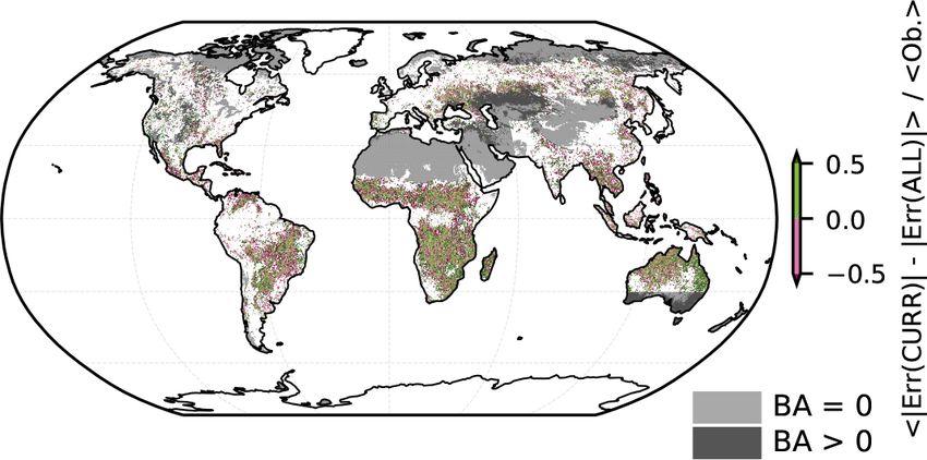
A. Kuhn-Régnier et al.: Importance of fuel-related vegetation properties
https://doi.org/10.5194/bg-18-3861-2021
Table 1. Characteristics of the datasets. End times as applicable to the processed data are indicated in brackets.
Variable Abbreviation Dataset Start End Time Reference
(mm-yyyy) (mm-yyyy)
Burnt area BA GFED4 06-1995 12-2016 monthly Giglio et al. (2013)
Diurnal temperature DTR ERA5 1950 present monthly Copernicus Climate Change Service (C3S)
range (12-2020) (2017)
Maximum temperature MaxT ERA5 1950 present monthly Copernicus Climate Change Service (C3S)
(12-2020) (2017)
Dry-day period DD ERA5 1950 present monthly Copernicus Climate Change Service (C3S)
(11-2020) (2017)
Soil moisture SWI Copernicus SWI 01-2007 11-2018 monthly Albergel et al. (2008); Wagner et al. (1999)
Lightning Lightning WGLC Lightning 01-2010 12-2018 monthly Kaplan and Lau (2019)
Above-ground tree AGB Tropical AGB: static static static Avitabile et al. (2016); Thurner et al. (2014)
biomass Avitabile, Northern
AGB: Thurner
Land cover (fractional CROP, SHRUB, ESA CCI Land Cover 1992 present yearly Li et al. (2018)
cover per grid cell) TREE, HERB (2019)
Solar-induced SIF GlobFluo SIF 01-2007 04-2015 monthly Köhler et al. (2015)
fluorescence
Vegetation optical VOD VODCA (Ku-band) 12-1997 12-2018 monthly Moesinger et al. (2019)
depth
Fraction of absorbed FAPAR MOD15A2H 02-2000 present monthly Myneni et al. (2015)
Biogeosciences, 18, 3861–3879, 2021
photosynthetically (03-2021)
active radiation
Leaf area index LAI MOD15A2H 02-2000 present monthly Myneni et al. (2015)
(11-2018)
Population density POPD HYDE 3.2 (updated) 2000 present yearly Klein Goldewijk (2017),
(2020) Kees Klein Goldewijk,
personal communication, February 2021
MCD64CMQ burnt MCD64 BA MCD64CMQ 11-2000 present monthly Giglio et al. (2018)
area (06-2020)
3864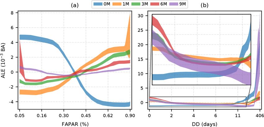
A. Kuhn-Régnier et al.: Importance of fuel-related vegetation properties                                                    3865

of snow cover and frozen soil for SWI and VOD (see e.g.            ticipate fires during the winter, having (by necessity of gap
Moesinger et al., 2020). There are also sporadic missing val-      filling) potentially unphysical values of SWI in the winter
ues in these datasets caused by for example cloud cover. Un-       should not affect results where relevant for our analysis.
fortunately, simple exclusion of the times lacking data is not
possible for our analysis because we commonly rely on an-          2.2.2    Interpolation
tecedent samples throughout. Thus, data gaps were filled us-
ing a two-step approach as in Forkel et al. (2017) in order to     All datasets were interpolated to a common 0.25◦ spa-
allow analysis of summer months at the affected locations.         tial grid. Datasets where the original spatial resolution was
This approach differentiates between two gap types based on        higher than this were averaged; the other datasets were
the amount of missing information for a specific month at          interpolated using nearest-neighbour interpolation to avoid
each location.                                                     smoothing local extrema (Forkel et al., 2017). Datasets that
    First, “persistent” gaps, defined as months for which 50 %     were only available at yearly time resolution (i.e. land cover,
or more of the observations across all years are missing, were     POPD) were linearly interpolated to monthly intervals. Tem-
filled using the minimum value observed at that location for       porally static data (i.e. AGB) were recycled. Processing was
the given predictor variable. We assume that this indicates        carried out before averaging to provide monthly climatolog-
missing data during the winter, since other causes for data        ical time series where applicable.
gaps (e.g. cloud cover) are predominantly “transient”. For ex-
                                                                   2.2.3    Antecedent predictor variables
ample, if a certain grid cell was missing data for more than
50 % of all Decembers in the record, these gaps in Decem-          The influence of antecedent conditions that might affect fuel
ber would be treated as persistent and therefore filled using      loads or fuel dryness, specifically vegetation properties and
minima.                                                            DD, on BA was investigated by using antecedent FAPAR,
    Second, the remaining transient gaps were filled using         LAI, VOD, SIF, and DD data from up to 2 years before
season-trend regression models with four harmonic terms            any given month (1, 3, 6, 9, 12, 18, 24 M, where M denotes
(k = 4) and without breakpoints. These models were fitted          months). The large autocorrelation between predictor vari-
using ordinary least squares regression to the entire time         ables could impede the visual interpretation of the impacts
series obtained during the first step, as mentioned before         of antecedent periods ≥ 1 year. Thus, anomalies were com-
using data from January 2008 to April 2015 (or Febru-              puted by subtracting the seasonal cycle relative to the desig-
ary 2000 to December 2019 for the monthly analysis). Cloud         nated month, resulting in the following transformations:
cover, which also affects detection in tropical and subtropi-
cal regions, is usually transient and therefore filled using the         (X 12 M) − (X 0 M) → X 112 M,
regression models. Locations where no observations were                  (X 18 M) − (X 6 M) → X 118 M,
available for > 52 months out of the total 88 months (re-
gardless of whether such data gaps always occurred in the          and (X 24 M) − (X 0 M) → X 124 M,
same month, as for persistent gaps, or at any point through-       where X ∈ {FAPAR, LAI, VOD, SIF, DD} and X 0 M refers
out the year) were discarded in a trade-off between data qual-     to the variable X in the current month. For example, the 12-
ity and geographic extent. For the monthly analysis, loca-         month antecedent X 12 M was transformed by subtracting
tions were discarded given > 138 unavailable months (out of        the instantaneous (month 0) value of X, thereby yielding the
239 months).                                                       anomaly in X, X 112 M, which may be easier to interpret.
    Use of a different gap-filling mechanism (Fig. S1b; tempo-
ral nearest-neighbour gap filling) yielded very similar results.   2.3     Machine-learning experiments
This simple nearest-neighbour gap-filling approach used for
the eventual ALL_NN model processes time series at a given         We used random forest (RF) regression to model the rela-
location, filling gaps by using the temporally closest avail-      tionships between BA and the driver variables (predictors).
able samples at that location. Of the two approaches, we de-       RF is an ensemble learning approach in which multiple de-
cided to use the season-trend model with minima filling be-        cision trees are constructed using a randomly sampled sub-
cause it represents a more physical solution; it is based on an    set of training observations. The final model is the aver-
approach previously used for vegetation variables (see Beck        age result from all of the individual decision trees. RF re-
et al., 2006), for which one would expect minima to occur          gression is highly suited to investigating the emergent con-
during winter. Indeed, as can be seen in Fig. S2, virtually        trols on fire because it is able to learn non-linear relation-
no samples are being filled with minima outside of winter          ships in high-dimensional space (Archibald et al., 2009).
and predominantly in the northern extreme latitudes. While         By averaging over multiple decision trees, RFs also miti-
our gap-filling methodology may yield unphysical values for        gate overfitting (Breiman, 2001). We used the scikit-learn
non-vegetation variables like SWI, we do not expect the fill-      version 0.24.1 (Pedregosa et al., 2011) RF regression im-
ing of SWI to have a big influence on the final results because    plementation in Python, with hyperparameters determined
we do not use antecedent values of SWI. Since we do not an-        using 5-fold random cross-validation (CV) of the eventual

https://doi.org/10.5194/bg-18-3861-2021                                                     Biogeosciences, 18, 3861–3879, 2021
3866 A. Kuhn-Régnier et al.: Importance of fuel-related vegetation properties
ALL model – n_estimators: 500, max_depth: 18 – We trained a number of different RF regression models to
and default values for all other parameters. The number test explicit hypotheses about the importance of antecedent
of estimators (n_estimators) determines the number of conditions on BA (see Table 2) using the defined hyperpa-
trees whose predictions are averaged. The maximum depth rameters on the climatological time series. The initial exper-
(max_depth) limits the number of split levels, which can iment (ALL) was run using the basic set of 15 predictor vari-
reduce overfitting. We also found that a limited number of ables related to climate, vegetation, and human influences on
split levels was necessary for the computation of SHapley fire (Table 1) and included both current and antecedent val-
Additive exPlanations (SHAP) values, although we expect ues of the four vegetation indices and DD, giving 50 predic-
this to be a limitation of the specific software we used as op- tor variables. A second experiment (TOP15) used only the 15
posed to the SHAP method itself. The hyperparameters were most important predictors from the ALL model, as a way of
only estimated once for the model containing all variables testing whether all the predictors were necessary and whether
due to computational constraints. including so many predictors resulted in overfitting.
The validation dataset was randomly sampled across space The choice of 15 predictors was heuristically based on the
and time and comprised 30 % of the data. To estimate how the slope of the feature importance plots (see Fig. S3), where, by
model will perform on unseen data, the out-of-bag (OOB) R 2 inspection, the importance change is minimal after 15 vari-
for the training dataset can be used (Fox et al., 2017). How- ables. Thereafter, no additional information was being con-
ever, since these data still belong to the training dataset, the veyed, so we decided to use this as our threshold. While use
R 2 for the validation dataset, which has not been used for of the more rigorous recursive feature elimination with cross-
variable selection or hyperparameter tuning, is also used to validation (RFECV) would be possible in principle, this com-
provide an alternative, independent, measure of the general- monly makes use of the Gini importance owing to its ease
isability of a given model. of calculation, as it only considers data already seen during
However, this is only valid if there is no autocorrelation be- training. Unfortunately, this also means that RFECV fails to
tween the samples. We investigated the degree of spatial au- account for overfitting, as it only considers the training data
tocorrelation using a variogram of global GFED4 BA, which when calculating feature importance (Meyer et al., 2019). In
informed a buffered leave-one-out (B-LOO) CV procedure contrast, the different approaches we jointly utilised to calcu-
following Ploton et al. (2020). This was carried out to deter- late a more robust feature importance metric are much more
mine how much the autocorrelation that may be present influ- computationally demanding, making RFECV infeasible.
ences the amount of potential overfitting. We did not employ All of the remaining experiments used combinations of
the extrapolation-prevention procedure used in Ploton et al. 15 predictor variables. The CURR experiment only used
(2020) because it led to the exclusion of significant areas like current-month values of each predictor. Therefore, compar-
northern Australia and west Africa. The B-LOO CV was ex- ison of the CURR and ALL experiments allowed the im-
ecuted as follows, where rmax = 50 pixels and Nt was chosen pact of including antecedent vegetation and moisture con-
such that the number of potential training samples was guar- ditions to be evaluated. However, some of the vegetation
anteed to be equal to or above Nt for all r ≤ rmax . predictors are highly correlated with one another, which
could artificially decrease their importance. To test this, we
1. Randomly choose a single location. The 12 monthly ran four further experiments (15VEG_FAPAR, 15VEG_LAI,
samples at this test location constitute the test set. 15VEG_VOD, 15VEG_SIF) that included the 10 most im-
2. Exclude samples from the potential training set in a cir- portant non-vegetation predictors from the ALL model, po-
cular region of radius r pixels around the test location, tentially including current and antecedent values of DD.
such that no potential training sample is closer than r In addition, each of these experiments contained one of
pixels to the test location. This limits the influence of the four vegetation predictors represented by both current
spatial autocorrelation. (month 0) and antecedent values (1, 3, 6, and 9 months).
To disentangle the effects of antecedent DD and antecedent
3. Randomly choose Nt training samples from all remain- vegetation properties, we ran a second set of vegetation
ing potential training samples. experiments (CURRDD_FAPAR, CURRDD_LAI, CUR-
RDD_VOD, CURRDD_SIF) where each vegetation predic-
4. Using a model trained on the above training samples, tor was represented by both current (month 0) and antecedent
predict BA for the test location. values (1, 3, 6, and 9 months) but only using current DD and
5. Increment r and repeat steps 1–4 until r has reached the next nine most important non-vegetation factors from the
rmax . CURR model. Finally, 5-fold random CV was used to iso-
late the best combination of the vegetation predictors under
This process was repeated 4000 times for each of the eight the constraint that each of the five states (0–9 months) must
linearly spaced investigated radii, with the lowest radius be- be represented exactly once (using any of the four vegetation
ing equal to 0. Due to computational constraints, the B-LOO predictors), resulting in the BEST15 model.
CV was only carried out for a single set of variables.
Biogeosciences, 18, 3861–3879, 2021 https://doi.org/10.5194/bg-18-3861-2021A. Kuhn-Régnier et al.: Importance of fuel-related vegetation properties 3867
In addition to the above climatological experiments, variable may be transferred to the correlated variables during
we also investigated monthly data for the time period the re-training process. The SHAP value (Lundberg and Lee,
November 2000–December 2029 (230 months) using the 2017; Lundberg et al., 2020) is the average of the marginal
15VEG_FAPAR_MON model. To avoid the temporal lim- contributions from a series of perturbations of the predictor
its of the GFED4 dataset (see Table 1) the MODIS variables. In a similar way to the PFI, this method shares
MCD64CMQ (Giglio et al., 2018) BA dataset was used. the importance amongst correlated predictor variables, which
Otherwise, this experiment uses the same variables as the may make them appear less significant than if they were in-
15VEG_FAPAR experiment with the exception of lightning, cluded on their own. SHAP values were computed for all val-
which was replaced with the similarly significant variable idation samples. In order to create a robust composite impor-
AGB (see Fig. S3) in order to enable processing of a longer tance metric for each predictor variable, we divided the Gini,
time period. In addition to 5-fold random CV as for the other PFI, LOCO, and SHAP metrics by the sum of their absolute
models, the performance and generalisability of this model values and then summed them.
was also measured using temporal CV. Here, the model was Maximally significant timescales were calculated by
trained on all samples excluding either all months within the weighting antecedent months using the largest SHAP value
years 2009–2012 (including 2012) or 2016–2019 (includ- magnitude out of all 12 months in the climatological data.
ing 2019). Thereafter, the R 2 was measured on whichever The maximum SHAP value magnitudes were calculated for
years were excluded for training. Note that unless explic- a predictor variable x at location ` on the latitude–longitude
itly specified, all following methodological descriptions will grid as follows:
relate to the climatological experiments as opposed to the
monthly 15VEG_FAPAR_MON experiment. SHAPx,` = SHAPx,`,mmax ,
where mmax = arg maxm∈{1,2,...,12} SHAPx,`,m . (1)
2.4 Measuring predictor importance and relationships
These were then used to calculate the maximally significant
Our goal is to determine the contribution of individual pre-
timescales for the basis predictor variable X (e.g. FAPAR)
dictors (including antecedent states of these predictors) to
using an average over antecedent months, a, weighted by
model skill at predicting BA and to examine the relation-
maximum SHAP value magnitudes:
ships between predictors and BA. There is no unique way
to measure the importance of a given predictor on model P
a,x a SHAPx,`
skill in predicting BA, and it is particularly difficult to as-
tmax,X,` = P
sign importance to individual predictors when there is a high
a,x SHAPx,`
degree of collinearity between them (Dormann et al., 2013; n
Nowack et al., 2018; Mansfield et al., 2020). We use four for a, x ∈ (0, X 0 M), (1, X 1 M), (3, X 3 M),
techniques to infer the importance of individual predictors: o
Gini impurity, permutation feature importance (PFI), leave- (6, X 6 M), (9, X 9 M) . (2)
one-column-out (LOCO), and SHAP values. The Gini impor-
tance aggregates the decrease in mean squared error (MSE) Locations with too many significant antecedent months
for each split involving a given predictor variable over the in- were ignored in order to visualise resulting relation-
dividual decision trees making up the RF. The PFI was calcu- ships more reliably; for example, if both the current
lated from five permutations of each predictor variable (val- (|SHAPX 0 M,` |) and 9-month antecedent (|SHAPX 9 M,` |)
idation set) using the ELI5 0.11.0 Permutation Importance magnitudes are dominant, the weighted mean month (accord-
(https://eli5.readthedocs.io/en/latest/index.html, last access: ing to Eq. 2) would lie in between, which is physically mean-
4 March 2021). While this provides an alternative assess- ingless. We designed an algorithm to detect SHAP values
ment of the prediction score, the permutations may result in that differ significantly from the baseline in order to miti-
unlikely or impossible combinations of predictors, and thus gate this. Additionally, we also applied a range-based thresh-
the PFI approach has a known tendency to overemphasise old, whereby locations were ignored if the variability of the
the importance of individual variables (Hooker and Mentch, SHAP values at location ` was below a threshold heuristi-
2019). The LOCO importance measure is estimated by re- cally related to the mean BA, BA` (based on all BA samples):
peatedly retraining the RF models, each time without one
particular predictor variable. The relative importance of this max SHAPx,` − min SHAPx,` < 0.12 × BA` . (3)
x x
predictor variable is then measured as the change in MSE
on the validation dataset, where a larger drop in MSE signi- We further used accumulated local effect (ALE) plots (Ap-
fies a larger significance for the variable within the dataset. ley and Zhu, 2020) to examine and interpret the coupled re-
The importance of correlated predictor variables may be un- lationships fitted by the RF models. ALE plots are a more
deremphasised in this approach since the model is retrained, robust alternative to partial dependence plots (PDPs) or indi-
and thus some of the importance associated with the removed vidual conditional expectation (ICE) plots (Apley and Zhu,
https://doi.org/10.5194/bg-18-3861-2021 Biogeosciences, 18, 3861–3879, 20213868 A. Kuhn-Régnier et al.: Importance of fuel-related vegetation properties
Table 2. The modelling experiments. Except for the ALL experiments, the other experiments included 15 predictor variables for compara-
bility. Differences in number of antecedent variables included in each experiment meant that different numbers of variables from the basic
set were used in these experiments. For the TOP15, 15VEG_X(_MON), and BEST15 models we used the most important variables from the
ALL experiment up to the required number of 15. For the CURRDD_X models, we used the most important non-vegetation variables from
the CURR model. Table S1 provides a detailed list of the variables included in each experiment.
Name No. Variables
ALL and ALL_NN 50 Basic set of current variables + current month and antecedent (1, 3, 6, 12, 18,
24 months) values for dry days and vegetation indices (FAPAR, LAI, VOD, SIF)
TOP15 15 Top 15 predictors from the ALL model
CURR 15 Only current values of the basic set of 15 variables
15VEG_X (e.g. 15VEG_FAPAR) 15 Top 10 non-vegetation variables from the ALL experiment, plus current and an-
tecedent (1, 3, 6, 9 months) vegetation index X (e.g. FAPAR)
CURRDD_X (e.g. CURRDD_FAPAR ) 15 Current and antecedent (1, 3, 6, 9 months) versions of the vegetation index X (e.g.
FAPAR), current DD, top nine other variables from the CURR experiment
BEST15 15 Current and antecedent DD, one current, 1, 3, 6, 9 months vegetation index (drawn
from the four potential vegetation indices) and five most important other variables
from the basic set
15VEG_FAPAR_MON 15 Same as the 15VEG_FAPAR experiment with monthly data instead of climatolog-
ical data and lightning data replaced by the next-most important non-vegetation
variable
2020; Molnar, 2020). We assessed the impact of each of
the predictor variables on BA in isolation using first-order
ALEs which take into account the effect of all other predic-
tor variables. However, underlying inhomogeneities may ap-
pear when the model fits different relationships for different
locations or times. We therefore tested for inhomogeneities
by subsampling the dataset prior to ALE plotting to enable
the visualisation of underlying relationships for a subset of
locations and times. The causes of these inhomogeneities
were explored using second-order ALE plots, which show
the combined effect of two predictor variables on BA.
3 Results and discussion Figure 1. Global climatological R 2 scores for the different ex-
periments. The CURR model is the only model that does not in-
In general, all models are able to predict BA using the given clude antecedent conditions, and it performs much worse as a re-
biophysical predictors. However, the inclusion of antecedent sult. Despite the fact that the ALL model contains 50 predictors,
predictors significantly improves model performance. Below, while all other models contain just 15, it does not perform signifi-
cantly better than the best models containing just 15 predictors (e.g.
we discuss the performance of the different models, the im-
15VEG_FAPAR). Note that although train R 2 scores are shown
portance of the different predictor variables, and their rela-
here, they are not indicative of model performance on unseen data,
tionships with BA. for which the shown train OOB scores should be used instead.
3.1 Model performance
The ALL model, which includes all 50 variables, achieves ative to observed BA is more widespread than underpredic-
an in-the-bag R 2 of 0.919 and out-of-bag (OOB) R 2 of tion (Fig. 2c). Nonetheless, there is no bias; the ALL model
0.701 for the training dataset and an R 2 of 0.701 for the predicts a mean out-of-sample BA of 2.54 × 10⁻³ compared
validation dataset (Fig. 1). Predictions on the validation set to the expected 2.48 × 10⁻³ . The apparent overprediction is
(Fig. 2b) show a similar geographic pattern to observed BA the result of plotting relative (as opposed to absolute) errors,
(Fig. 2a). However, overprediction in the validation set rel- which amplifies the fact that the ALL model does not predict
Biogeosciences, 18, 3861–3879, 2021 https://doi.org/10.5194/bg-18-3861-2021A. Kuhn-Régnier et al.: Importance of fuel-related vegetation properties 3869
not appear to occur given the stochastic nature of the training
process. Failure to capture extreme events well is likely due
to their rarity, resulting in the absence of comparable training
data (see also e.g. Joshi and Sukumar, 2021).
Using a combination of regional neural networks trained
on fewer variables at a coarser spatial resolution of 1◦ × 1◦ ,
Joshi and Sukumar (2021) found a global R 2 score for BA
prediction of 0.36. An earlier study by Thomas et al. (2014)
considered an R 2 score of 0.6 as indicating a robust pre-
diction. Our results compare favourably to both. To further
ensure model robustness, we also compared the PFI impor-
tances computed separately on the training and validation
sets in Fig. S6. There is no appreciable difference between
the two, which is indicative of a lack of overfitting, since
the model training has not unduly prioritised certain vari-
ables based on the training set (Dankers and Pfisterer, 2020).
Additionally, using the variogram shown in Fig. S7, we car-
ried out the B-LOO CV as detailed in Sect. 2.3 in order
to investigate the influence of spatial autocorrelation on the
15VEG_FAPAR model (see Fig. S8). The performance of
the model drops as a larger region around the test samples
is excluded (with 30 pixels corresponding to ∼ 900 km at
the Equator, which is the scale of autocorrelation identified
using Fig. S7). However, as opposed to the case study in Plo-
ton et al. (2020), the R 2 score plateaus at around 0.1–0.4
beyond ∼ 900 km instead of dropping to 0, thereby indicat-
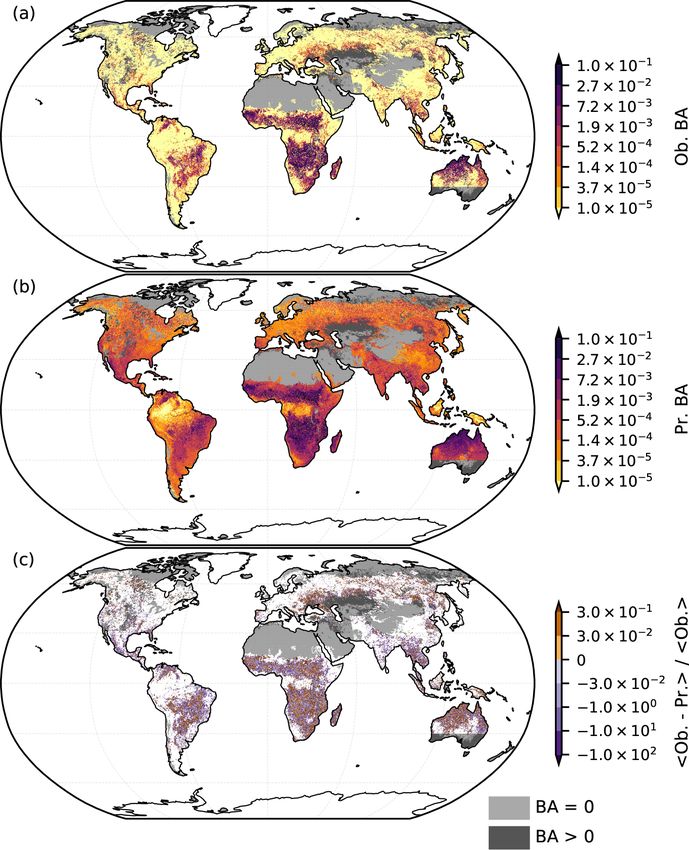
Figure 2. (a) Average observed (Ob.) BA derived from the GFED4 ing the robustness of our model. Certain regions and extreme
BA dataset (Giglio et al., 2013). (b) Out-of-sample predictions (Pr.) events are poorly captured by the model, accounting for the
by the ALL model on the validation dataset. (c) Relative prediction lower end of this range. Furthermore, the model is potentially
error of the ALL model calculated by taking the mean of the differ-
forced to extrapolate to a larger extent as the exclusion radius
ence between observations and predictions divided by the mean ob-
is increased, leading to an overly pessimistic performance
servations. While the predictions in panel (b) are qualitatively very
similar to the observations in panel (a), there is an overestimation of estimate. The extrapolation-prevention procedure in Ploton
low BA. Areas with very low or 0 observed BA (a) are omitted from et al. (2020) was not used here because it led to the exclusion
panel (c) to avoid division by (nearly) 0. Despite the visual exag- of certain key regions.
geration of the errors, which are generally small, there is no overall
pattern. Note that sharp data availability boundaries (e.g. in western 3.2 Importance of predictors
Asia, southern Australia) are introduced by the AGB dataset. Grey
shading indicates regions with fire data availability, but where one Climate variables and fuel-related vegetation indices have
or more of the other datasets is not available. Light grey indicates the strongest influence on BA in the ALL model (Table S2).
regions where mean BA is 0, with dark grey representing regions Both current and antecedent conditions are important. Cur-
with non-zero mean BA.
rent DD and MaxT are ranked first and fifth respectively,
but antecedent DD also has a moderate influence (DD 1 M
and DD 3 M are ranked 10th and 13th in importance, respec-
very low BA accurately; out-of-sample BA predictions are tively). Similarly, although current FAPAR is the most im-
no lower than 7.39 × 10⁻⁷ , while the observed BA is 0 for portant vegetation index (second), with both current SIF and
85.7 % of samples. Generally, the model captures intermedi- VOD occurring in the top 15 predictors, antecedent vegeta-
ate BA better than extreme BA, leading to overprediction at tion state also has a strong influence on BA. However, an-
low and underprediction at high BA values. Thus, more sam- tecedent conditions > 9 months are unimportant in the ALL
ples are over-predicted because there are more values with model. Vegetation characteristics such as the cover of spe-
low BA than high BA, leading to many instances of slight cific plant types (TREE, SHRUB, HERB) and AGB are only
overprediction balanced by few instances of comparatively moderately important in determining BA (all ranked below
large underprediction (Figs. S4, S5). The model may strug- the top 15 predictors). Human impacts, as represented by
gle to predict 0 BA because the random forest model consists CROP and POPD, are also only moderately important glob-
of many smaller decision trees. All 500 individual models ally for BA, ranked respectively 8th and 15th. Natural igni-
would have to predict 0 to yield this value overall, which does tions as represented by lightning are only ranked 21st, sug-
https://doi.org/10.5194/bg-18-3861-2021 Biogeosciences, 18, 3861–3879, 20213870 A. Kuhn-Régnier et al.: Importance of fuel-related vegetation properties
gesting that at a global climatological scale burning is not
limited by lightning.
The finding that fuel build-up on timescales longer than
a year is not an important predictor of BA may initially be
surprising given that fuel build-up as a result of fire suppres-
sion has been linked to large and catastrophic fires (e.g. in
the USA; Marlon et al., 2012; Parks et al., 2015; Higuera
et al., 2015). The failure to detect an influence of longer-
term fuel build-up on BA probably reflects the short time
interval (1–2 years) considered for antecedent fuel build-
up, far shorter than the timescales of coarse fuel build-up
in these ecosystems. The seasonal differences captured by Figure 3. Mean change in out-of-sample prediction error be-
our analyses may also be unimportant in regions where long tween the CURR and ALL models, relative to mean observations
fire-return times (or fire suppression) allow fuel build-up (). Green regions have decreased prediction error using the
over longer periods. Wetter forests with long fire-return in- ALL model compared to the CURR model, and vice versa for the
tervals may also be more affected by longer-term moisture purple regions. Areas with high BA (see Fig. 2a) tend to experience
lower changes in relative prediction error. Areas with very low or 0
deficits (Abatzoglou and Kolden, 2013) that are not captured
observed BA (see Fig. 2a) are omitted to avoid division by (nearly)
in the limited time period analysed. However, van der Werf 0. Note that sharp data availability boundaries (e.g. in western Asia,
et al. (2008) used 13 months of fuel accumulation before southern Australia) are introduced by the AGB dataset. Grey shad-
the peak of the fire season to investigate herbaceous fuels, ing indicates regions with fire data availability, but where one or
which supports our findings somewhat. It would be worth- more of the other datasets is not available. Light grey indicates re-
while to re-examine the influence of longer timescales on gions where mean BA is 0, with dark grey representing regions with
BA when longer datasets are available, as, even when con- non-zero mean BA.
sidering the ∼ 20-year long MODIS record (which we do
using the 15VEG_FAPAR_MON model), we are strongly
limited by the data available to us. Predictability in boreal olutions, the lack of accurate, reliable fire statistics at finer
ecosystems is expected to remain very limited because the scales (Abatzoglou and Kolden, 2013) limits the temporal
return times are many times longer than the time series, so and spatial resolution that can usefully be achieved.
there is a very large stochastic component. The lower perfor- Although the limitation of the spatial (and temporal) res-
mance of our monthly 15VEG_FAPAR_MON model with olution of the observations could impact the realism of
over 19 years of data, presented further below, in addition our models, as could the omission of variables that affect
to the limited predictability of boreal regions found by Joshi fuel build-up, the consistency of the vegetation relationships
and Sukumar (2021) despite their use of 14 years of data, shown by all the models (as detailed below) including an-
both support this. tecedent conditions indicates that processes related to fuel
Our analyses are also impacted by the influence of previ- build-up are adequately represented by the chosen set of pre-
ous fires on current vegetation conditions. Burnt grid cells dictors. The different importance metrics used are also in
could have a lower FAPAR, for example, as a result of prior broad agreement, especially regarding the most important
burning within the current month. This is a problem because predictors like FAPAR and DD (see Fig. S1).
we are solely interested in how pre-fire vegetation conditions
affect BA. The temporal and spatial scales of the analysis are 3.3 Models with fewer predictors
responsible for this: a monthly analysis cannot resolve pro-
cesses that occur on the order of days. Further, the impact The model using the top 15 predictors from the ALL model
of previous fires on spatially averaged vegetation properties (TOP15) performs only marginally worse than the ALL
is expected to be proportional to the burnt fraction of the af- model, with an in-the-bag R 2 of 0.919 and out-of-bag (OOB)
fected grid cell. In savannah regions of Africa and northern R 2 of 0.688 for the training dataset and an R 2 of 0.685 for
Australia, where on the order of 10 % of a 0.25◦ grid cell the validation dataset. This nearly equivalent performance re-
may burn in a given month, this could have a significant ef- flects the fact that there is a high degree of correlation be-
fect on the averaged values of vegetation properties used in tween several of the variables (Fig. S9) included in the ALL
our analyses. Analysis using a finer spatial scale would coun- model, while also implying that the inclusion of extra predic-
teract this spatial smoothing by allowing burnt pixels to be tors in the ALL model does not improve predictive capabil-
ignored so that predictor values may be estimated only from ity. Therefore, this shows that it is not necessary to include
unburnt cells. Using a finer temporal resolution would al- multiple fuel-related vegetation variables in order to predict
low the calculation of predictor variables only up to the time BA, provided that both current and antecedent conditions are
of burning. In practice, however, while many variables (e.g. taken into consideration. The removal of predictor variables
MODIS-based vegetation variables) are available at finer res- is however likely to reduce overfitting in the TOP15 model
Biogeosciences, 18, 3861–3879, 2021 https://doi.org/10.5194/bg-18-3861-2021A. Kuhn-Régnier et al.: Importance of fuel-related vegetation properties 3871
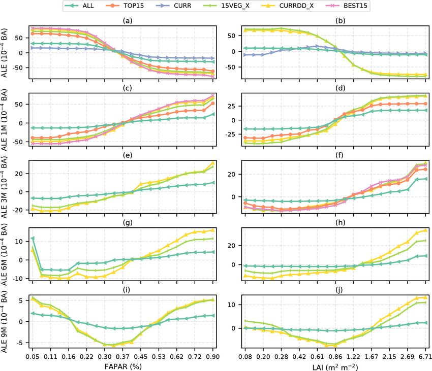
Figure 4. First-order ALEs for different antecedent (0 M, 1 M, 3 M, 6 M, and 9 M, where M denotes months) relationships with (a) FAPAR
and (b) DD in the 15VEG_FAPAR model, showing the underlying relationships with BA after accounting for all other variables. The shaded
regions represent the standard deviation around the mean of 100 ALEs each using 122 567 random samples of the training data (∼ 10 %).
Evenly spaced quantiles were used in the construction of the plots. Labels were calculated using the averaged quantiles of all the variables
used. A clear difference between instantaneous and antecedent relationships can be seen in both cases, with instantaneous FAPAR limiting
BA while antecedent FAPAR promotes BA, and vice versa for the dry-day period. Note that the enhancement of BA due to extreme droughts
(extreme dry-day period) is apparent across time periods.
compared to the ALL model (Runge et al., 2019; Nowack CURR model (Fig. 1), only the 15VEG_FAPAR model per-
et al., 2020; Joshi and Sukumar, 2021). forms similarly to the TOP15, BEST15, and ALL models.
Thus, considered on its own, FAPAR is the best fuel-related
3.3.1 Importance of antecedent fuel-related predictors vegetation predictor, followed by LAI, SIF, and then VOD
(Fig. 1). However, all four fuel-related vegetation predictors
The importance of antecedent fuel-related vegetation indices produce reasonable results, and other predictors (e.g. VOD)
for predicting BA is corroborated by the results from the have been found to be important in other studies (e.g. Forkel
model that only includes predictors for the current month et al., 2017).
(CURR), where there is a large decrease in the R 2 for the The importance of including antecedent DD is borne out
validation dataset compared to either the ALL (−0.123) or by the comparison of these four experiments and the experi-
TOP15 (−0.107) model. The decrease in the R 2 for the ments which only included current DD (CURRDD_FAPAR,
training dataset is smaller (−0.042) than for the validation CURRDD_LAI, CURRDD_VOD, CURRDD_SIF). In each
dataset, indicating that overfitting may be more of a prob- case, the predictions for the same vegetation predictor vari-
lem in the CURR model than the ALL model. Analysis of able are worse (Fig. 1).
the mean out-of-sample prediction error shows that 54.7 % The BEST15 model contains the best combination of the
of grid cells are better predicted in the ALL model compared fuel-related vegetation predictors (current FAPAR, FAPAR
to the CURR model (Fig. 3). The performance improvements 1 M, LAI 3 M, SIF 6 M, SIF 9 M), determined by optimising
(from the CURR to the ALL model) also tend to have a larger their timescales. This suggests that FAPAR is most important
magnitude than the performance decreases, contributing to on short timescales (current, 1 month) with the other vegeta-
the improvement in the global R 2 score. Compared to the tion properties appearing to be more useful on longer time
ALL model, fuel-related vegetation properties are less im- frames. The performance of this model, with a training R 2 of
portant in the CURR model: VOD is the highest-ranked veg- 0.925 and a validation R 2 of 0.691, is only bettered by the
etation variable but is only fourth in importance (Table S2). ALL model. The good performance of models including FA-
The four fuel-related vegetation variables included in the PAR is due to the fact that the parts of the world responding
TOP15 model are correlated with one another (Fig. S9), es- most strongly to FAPAR 0 M and FAPAR 1 M tend to be fuel-
pecially on specific antecedent timescales. This suggests it limited, dry biomes accounting for the majority of global
may be unnecessary to include all these variables to cap- BA (Giglio et al., 2013). Therefore, globally averaged model
ture the influence of fuel build-up on BA. Comparison of the performance metrics will tend to favour predictor variables
models which only include current and antecedent conditions which best represent these dominant fire regimes. This is sup-
for one fuel-related vegetation variable (15VEG_FAPAR, ported by previous analyses which have found predictability
15VEG_LAI, 15VEG_VOD, 15VEG_SIF) confirms this. in regions with infrequent fires like boreal regions or Europe
However, while all these models perform better than the
https://doi.org/10.5194/bg-18-3861-2021 Biogeosciences, 18, 3861–3879, 20213872 A. Kuhn-Régnier et al.: Importance of fuel-related vegetation properties
Figure 5. First-order ALEs for different lags (< 1 year) from all relevant modelling experiments for the relationships between BA and
FAPAR (left-hand column) and LAI (right-hand column). Evenly spaced quantiles were used in the construction of the plots. Notably, the
relationship between LAI and BA is not modelled consistently by the CURR model (b), but relationships with BA are generally consistent
across models otherwise.
to be poor in contrast to regions with more frequent fires (e.g. Current DD has a positive effect on BA (Fig. 4b), while
Joshi and Sukumar, 2021). antecedent DD has a generally negative effect except if DD
is very high when the effect becomes positive again. Whereas
the positive antecedent effect of FAPAR on BA is strongest
3.4 Current and antecedent relationships with BA for the preceding 1-month relationship and then gets weaker,
the negative impact of antecedent DD becomes gradually
Current and antecedent states of both fuel-related vegetation stronger up to 9 months. In contrast to FAPAR, dry condi-
properties and DD have different impacts on BA (Fig. 4). tions in the current month promote fire, whereas dry con-
Current FAPAR has a negative effect on BA, while an- ditions in preceding months reduce vegetation growth and
tecedent FAPAR has a positive effect on BA (Fig. 4a). The hence fuel build-up. Although prolonged droughts might be
importance of current FAPAR changes most rapidly at in- expected to reduce the availability of fuel, the (on average)
termediate levels of FAPAR. The impact of antecedent FA- positive relationship between BA and DD at very high lev-
PAR is strongest for the preceding 1 month but persists for els of DD across all antecedent states does not support this
up to 6 months; longer lags tend to produce results more sim- expectation. The positive impact of drought in the current
ilar to the current relationship because of autocorrelation at month becomes apparent for dry days >∼ 10 d, whereas the
the yearly scale. These relationships make intuitive sense: threshold is higher for antecedent months: BA only increases
whereas high antecedent levels of FAPAR suggest that fuel when the number of dry days is >∼ 20 d for the preceding
availability is not a limiting factor, high FAPAR in the current month (DD 1 M) and requires >∼ 40 d for DD 9 M. This
month indicates that the vegetation has sufficient moisture to suggests that positive large antecedent DD may reflect pro-
be actively growing and is therefore less likely to burn.
Biogeosciences, 18, 3861–3879, 2021 https://doi.org/10.5194/bg-18-3861-2021You can also read