PHD THESIS JAN KREMER - ACTIVE AND ADAPTIVE LEARNING FROM BIASED DATA WITH APPLICATIONS IN ASTRONOMY
←
→
Page content transcription
If your browser does not render page correctly, please read the page content below
UNIVERSITY OF COPENHAGEN
FACULTY OF SCIENCE

 PhD thesis
 Jan Kremer

 Active and Adaptive Learning from Biased
 Data with Applications in Astronomy

 Supervisor: Christian Igel

 Submitted: 10/06/2016
Summary

    This thesis addresses the problem of machine learning from biased
datasets in the context of astronomical applications. In astronomy there are
many cases in which the training sample does not follow the true distribution.
The thesis examines different types of biases and proposes algorithms to
handle them.
    During learning and when applying the predictive model, active learning
enables algorithms to select training examples from a pool of unlabeled
data and to request the labels. This allows for selecting examples that
maximize the algorithm’s accuracy despite an initial bias in the training set.
Against this background, the thesis begins with a survey of active learning
algorithms for the support vector machine.
    If the cost of additional labeling is prohibitive, unlabeled data can
often be utilized instead and the sample selection bias can be overcome
through domain adaptation, that is, minimizing the discrepancy between
training sample and the true distribution. A simple method consists of
weighting the elements of the training sample such that the empirical risk
becomes an unbiased estimator of the true distribution’s risk. The respective
weights can be computed as the probability density ratio of training and test
distribution. A model selection criterion—which is known in the context
of kernel-based weight estimators—is proposed to be combined with a
nearest neighbor density ratio estimator. It is shown to compare favorably
to alternative approaches when applied to large-scale problems with low-
dimensional feature spaces: a common setting in astronomical applications
such as photometric redshift estimation.
    Another form of bias stems from label noise. This thesis considers the
scenario in which unreliable labels can be replaced by highly accurate labels
at a certain cost. This is, for example, the case in crowd-sourcing, where
unreliable labelers can be corrected by experts, or in astronomy, where
a labeling based on photometric data can be improved by spectroscopic
observations. An algorithm to actively select objects for correction under a
limited re-labeling budget is presented. It is shown empirically to converge
faster to the maximally attainable accuracy than the state-of-the-art.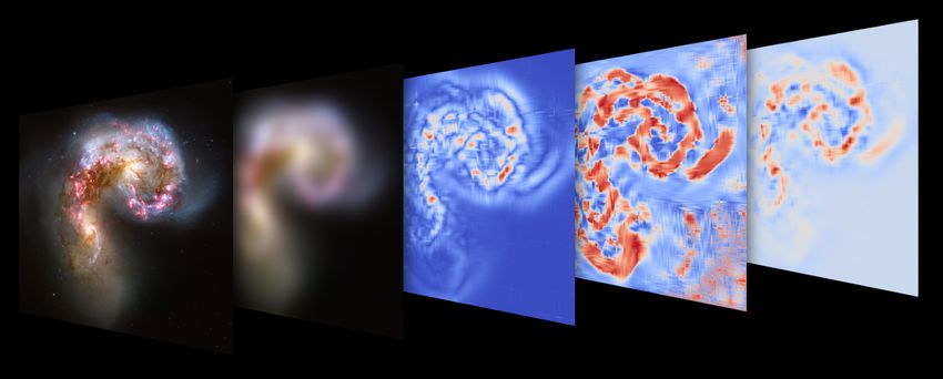
Acknowledgments

This thesis would not have been possible without the help of many people, the
most important of whom I would like to mention here. First and foremost, I
thank my supervisor Christian Igel. He was always available for stimulating
discussions and encouraged me when things failed. The diverse collection of pens
he forgot on my desk bears witness to his constant support. I would also like
to thank Kim Steenstrup Pedersen for serving as my second supervisor and for
helping me whenever I needed it.
    I thank Fei Sha for hosting me in his group at UCLA and for the great
discussions we had. His enthusiasm for science is truly inspiring. Furthermore, I
would like to thank my colleague Fabian Gieseke for his constant encouragement,
and helping me especially in the beginning of this endeavor.
    I thank my colleagues and office mates Niels Dalum Hansen, Oswin Krause
and Kristoffer Stensbo-Smidt for great scientific and non-scientific discussions,
blackboard sessions and comedy. Many thanks to Susan Nasirumbi Ipsen for
helping me with administrative matters and the rest of the image section for
making this a nice place to work at.
    I thank my parents Otto and Margret for always supporting any of my
interests. Last but not least, I would like to thank my girlfriend Adriana Ion for
putting things into perspective and for being there for me.
    I would also like to acknowledge the Danish Council for Independent Research
for supporting this work through the project “SkyML”.

                                        3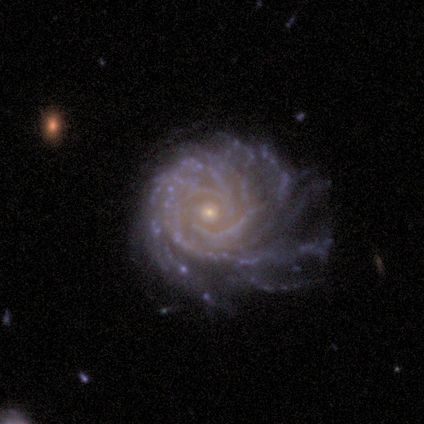
Contents

Contents                                                                                               4

1 Introduction                                                                                         7
  1.1 Active Learning . . . . . . . . . . . . . . . . .   .   .   .   .   .   .   .   .   .   .   .    9
  1.2 Domain Adaptation . . . . . . . . . . . . . .       .   .   .   .   .   .   .   .   .   .   .   10
  1.3 Learning with Noisy Labels . . . . . . . . . .      .   .   .   .   .   .   .   .   .   .   .   11
  1.4 Active Label Correction . . . . . . . . . . . .     .   .   .   .   .   .   .   .   .   .   .   11
  1.5 Outline of the Thesis . . . . . . . . . . . . . .   .   .   .   .   .   .   .   .   .   .   .   12
  1.6 Included Manuscripts and Published Articles         .   .   .   .   .   .   .   .   .   .   .   12

2 Big Universe, Big Data: Machine Learning and Image                              Analy-
  sis for Astronomy                                                                                   13
  2.1 Introduction . . . . . . . . . . . . . . . . . . . . . . . . .              .   .   .   .   .   13
  2.2 Ever-Larger Sky Surveys . . . . . . . . . . . . . . . . . .                 .   .   .   .   .   14
  2.3 Big Data Analysis in Astronomy . . . . . . . . . . . . .                    .   .   .   .   .   17
  2.4 Astronomy Driving Data Science . . . . . . . . . . . . .                    .   .   .   .   .   18
  2.5 Physical Models vs. Machine Learning Models . . . . .                       .   .   .   .   .   22
  2.6 A Peek into the Future . . . . . . . . . . . . . . . . . . .                .   .   .   .   .   23

3 Active Learning with Support Vector Machines                                                        25
  3.1 Introduction . . . . . . . . . . . . . . . . . . . . . .        .   .   .   .   .   .   .   .   25
  3.2 Active Learning . . . . . . . . . . . . . . . . . . . .         .   .   .   .   .   .   .   .   26
  3.3 Support Vector Machine . . . . . . . . . . . . . . .            .   .   .   .   .   .   .   .   27
  3.4 Uncertainty Sampling . . . . . . . . . . . . . . . .            .   .   .   .   .   .   .   .   29
  3.5 Combining Informativeness and Representativeness                .   .   .   .   .   .   .   .   35
  3.6 Multi-Class Active Learning . . . . . . . . . . . . .           .   .   .   .   .   .   .   .   40
  3.7 Efficient Active Learning . . . . . . . . . . . . . . .         .   .   .   .   .   .   .   .   42
  3.8 Conclusion . . . . . . . . . . . . . . . . . . . . . .          .   .   .   .   .   .   .   .   43

4 Nearest Neighbor Density Ratio Estimation for Large-Scale
  Applications in Astronomy                                                                           45
  4.1 Introduction . . . . . . . . . . . . . . . . . . . . . . . . . . . . . .                        46
  4.2 Kernel-based Density Ratio Estimation . . . . . . . . . . . . . .                               47
  4.3 Nearest Neighbor Density Ratio Estimation Revisited . . . . . .                                 48
  4.4 Experiments . . . . . . . . . . . . . . . . . . . . . . . . . . . . . .                         51
  4.5 Conclusion . . . . . . . . . . . . . . . . . . . . . . . . . . . . . .                          54

                                         4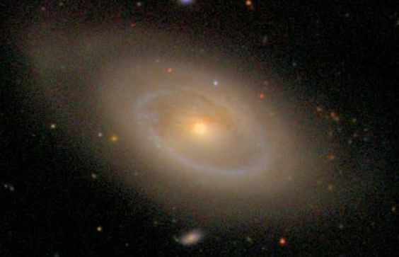
Contents                                                                            5

5 Active Label Correction for Class-Conditional Noise                              57
  5.1 Introduction . . . . . . . . . . . . . . . . . . . . . . . . .   . . . . .   57
  5.2 Active Label Correction by Maximizing Expected Model             Change      59
  5.3 Active Label Correction with Logistic Regression . . . .         . . . . .   61
  5.4 Active Label Correction with Softmax Regression . . . .          . . . . .   65
  5.5 Estimating the Noise Rates . . . . . . . . . . . . . . . .       . . . . .   67
  5.6 Experiments . . . . . . . . . . . . . . . . . . . . . . . . .    . . . . .   68
  5.7 Conclusion . . . . . . . . . . . . . . . . . . . . . . . . .     . . . . .   70
  5.8 Additional Experiments . . . . . . . . . . . . . . . . . .       . . . . .   71

6 Conclusion and Future Work                                                       79

Bibliography                                                                       81
Chapter 1

Introduction

In many application areas the available datasets violate a basic assumption
underlying most supervised machine learning algorithms: Training and test data
are not drawn from the same distribution, that is, we have a sample Strain of
labeled examples (x, y) drawn from a distribution ptrain , which is different from
the test distribution ptest . We aim at learning a hypothesis h from Strain which
minimizes the generalization error over ptest . In general, if ptrain and ptest are
unrelated, this is not possible. In this thesis, we will consider scenarios in which
this difference is caused by a biased sample selection or by noisy labeling. We
show that if we make certain assumptions on the type of bias or label noise, or
have the possibility to obtain additional labels, we can still learn from biased
training data.
    In astronomy, biased datasets are common. High-quality measurements that
provide ground-truth labels are costly and only available for certain regions of
the input space. This creates a sample selection bias. Furthermore, certain
annotations have to be performed by human labelers who are often unreliable or
make systematic errors. Learning algorithms which fail to address these biases
will in many cases perform sub-optimally.
    Suitable bias correction strategies depend on the type of bias and on the
acquisition costs. If we can afford to take additional measurements, we can select
candidates for observation by active learning—a learning method which chooses
the examples it finds most useful to learn from. This has two advantages. First,
we may need to only examine a fraction of examples in comparison to sampling
uniformly at random from Strain . Second, we can compensate for a selection bias
by selecting examples that are under-represented in the current training set Strain
with respect to ptest .
    Often, however, it is not possible to label additional examples, for instance,
because annotation costs are prohibitive. Each example might have to be exam-
ined by an expert or additional expensive measurements are needed to derive
the correct label. An example from astronomy is redshift estimation. The red-
shift of a galaxy measures how much its observed wavelength is shifted towards
longer wavelengths. We can use spectroscopy, which measures the photon count
over a wide range of wavelengths, to determine the redshift with high precision.
Spectroscopy, however, is very time-consuming, it can only measure few objects

                                         7
8 Chapter 1. Introduction
at the same time, and its depth is limited. It is therefore very costly and the
measurements are biased towards observations closer to the observer.
Photometric measurements, which measure an object’s intensity in a few
bands, provide an inexpensive alternative to spectroscopy. As they only require
an image of the sky, many objects can be observed at the same time. Photometric
data is also available for objects at great distance to the observer, but has the
drawback of providing less information in comparison to spectroscopic data.
Building a photometric redshift model based on known photometry-spectroscopy
correspondences remains a challenge in astronomy. It is complicated by the
selection bias caused by spectroscopic observations.
If an unlabeled sample drawn from ptest is available at training time, we can
minimize the discrepancy between training and test set by importance-weighting.
This is a simple strategy that re-weights training examples so that the empirical
risk of h on Strain becomes an unbiased estimator of the risk over the test
distribution ptest . The respective weights can be computed as the probability
density ratio between ptrain and ptest .
In some cases, expert annotations can be replaced by crowd-sourcing the
labeling process. A successful example in the astronomical domain is the Galaxy
Zoo project.1 It collected millions of labels from volunteers who classified images
observed by the Sloan Digital Sky Survey (SDSS) telescope and the Hubble Space
Telescope. The task was to determine the galaxy’s morphology which describes
its visual appearance, for instance, whether it looks elliptical or spiral.
While crowd-sourcing provides an inexpensive mechanism to collect a large
number of labels, the accuracy may suffer due to missing knowledge or low
motivation of the annotators. But even when experts obtain the labels, the
quality of the annotation is ultimately limited by the quality of the observation.
Figure 1.1 shows an example of a galaxy observed by the ground-based SDSS
telescope and by the space-based Hubble telescope. While an annotator might
label this galaxy as elliptical based on the left image, it is clear from the right
image, that it is in fact a spiral. When a new telescope becomes available, simply
using a label which is based on an old measurement would not provide the
most accurate annotation given the new observation. Both crowd-sourcing and
low-quality measurements thus can lead to label noise.
The effect of label noise can be mitigated by minimizing a surrogate loss
which takes into account a noise model. A simple and well-studied noise model
is class-conditional label noise. It assumes that the probability of observing the
wrong label is independent of the observed example given the true label. While
this assumption is most likely violated in many real-world classification tasks, it
has the advantage that the number of model parameters only depends on the
number of classes. This makes it easier to learn than sample-dependent noise
models.
In addition to using a label-noise robust model, one way to mitigate label noise
is simply to correct false labels manually. In practice the number of corrections is
usually limited by annotation costs. Active label correction aims at correcting the
1
Visit http://www.galaxyzoo.org to classify a few galaxies yourself.1.1. Active Learning 9
(a) Ground-based SDSS telescope (b) Hubble Space Telescope
Figure 1.1: A spiral galaxy as imaged by the Sloan Digital Sky Survey (SDSS)
ground-based telescope on the left and by the Hubble Space Telescope on the
right. Due to the lack of atmospheric distortion, the Hubble image is much better
resolved and reveals the spiral character of the galaxy. An annotator would label
this galaxy most likely as an elliptical if they based their annotation on the left
image [Galaxy Zoo, 2012].
label which increases the accuracy of the classifier the most to lessen annotation
costs. In the following we will present the background of the aforementioned
concepts in more detail.
1.1 Active Learning
Active learning aims at optimally utilizing a limited budget for acquiring labeled
data for supervised learning [Hanneke, 2009, Settles, 2012]. In many practical
applications data are not scarce, but labels are. Acquiring them is costly, and,
thus, the limited budget should be spent on labels that provide the maximum
insight to the learning algorithm. It has been shown empirically and theoretically
that in many cases one can do better than passive learning, that is, sampling
uniformly at random from the training set [Beygelzimer et al., 2010].
Another case in which active learning can be beneficial is large-scale learning.
Even if large amounts of labeled data are available, running time constraints
may not allow for training on the entire set. By exploiting informative regions
of the input space, performance gains over passive learning can be achieved. In
addition, active learning can mitigate the effects of a sample selection bias by
choosing examples that balance misrepresentation in the training set [Richards
et al., 2012].
Any active learning strategy necessarily has the drawback that the acquired
sample is not independent and identically distributed (i.i.d), an assumption which10 Chapter 1. Introduction
underlies most supervised learning algorithms. Luckily, this bias is introduced by
the learner itself and can thus be controlled, for instance, by importance-weighting
[Sugiyama, 2005, Bach, 2006, Beygelzimer et al., 2009]: If an example is selected
with too high probability it receives a small weight and vice versa, if it is sampled
with too small probability it receives a large weight.
Support vector machines exhibit excellent empirical performance while being
well-understood theoretically [Cortes and Vapnik, 1995, Steinwart and Christ-
mann, 2008]. Due to their limited scalability to large datasets they can benefit
greatly from active learning. Moreover, they can inform active learning strategies
by providing a distance to the separating hyperplane as a measure of how infor-
mative an example is [Lewis and Gale, 1994b, Tong and Chang, 2001]. To correct
a selection bias, sample weights can be introduced easily [Zadrozny et al., 2003].
1.2 Domain Adaptation
If there is no budget available to acquire additional labels, we can instead utilize
unlabeled data. If we have access to a large sample of unlabeled data that follows
the distribution of the test sample ptest , we can apply unsupervised domain
adaptation techniques [Daume III and Marcu, 2006, Jiang, 2008]. These aim
at minimizing the discrepancy between the marginal distributions ptrain (x) and
ptest (x) of training and test data [Ben-David et al., 2006].
As in active learning, importance weights can be used to alleviate the selection
bias [Huang et al., 2007, Cortes et al., 2008]. By weighting examples in the training
set by the probability density ratio of ptest to ptrain , an unbiased estimate of the
true risk can be computed. As in this case the weights are solely determined by
the data and not controlled by the algorithm as in active learning, the variance
of the estimator has to be controlled with care [Cortes et al., 2010].
The naive solution is estimating the probability densities separately before
computing their ratio. Sugiyama et al. [2010b] show empirically that this leads
to sub-optimal results. This might be because a small error in the estimation of
the denominator density can lead to a large error in the estimated ratio. Several
authors have proposed to use a one-step procedure to estimate the importance
weights directly [Sugiyama et al., 2008, Bickel et al., 2009]. Most estimators in
the literature rely on kernel-based methods [Huang et al., 2007, Kanamori et al.,
2012, Izbicki et al., 2014]. When applied to large-scale datasets these require
sub-sampling or approximations.
Nearest neighbor-based algorithms constitute a conceptually simple alternative
to kernel-based estimators [Lima et al., 2008, Loog, 2012]. They perform well
when the dimensionality of the input space is low and sample sizes are large,
a scenario which is common in astronomical applications such as photometric
redshift estimation [Lima et al., 2008]. They rely on counting test examples
within a radius that is defined by the Kth neighbor in the training sample,
thereby flexibly handling sparse regions in the input space.1.3. Learning with Noisy Labels 11
1.3 Learning with Noisy Labels
Apart from sample selection bias, datasets may be affected by label noise [Frenay
and Verleysen, 2014]. For instance, labels which are annotated by non-experts
through crowd-sourcing are often unreliable [Raykar et al., 2010]. Even though
these effects can be mitigated by a weighted averaging or by modeling the labelers,
a certain amount of data will remain labeled incorrectly. Furthermore, even
expert labelers may have difficulties annotating examples which are not well
resolved, or belong to a class that is easily confused with another. For example,
in astronomy the quality of observations is influenced by weather conditions,
resolution and other factors. In the case of galaxy morphology classification,
an object that has been identified in an astronomical survey as an elliptical
galaxy might in fact be a spiral. The particular details that would have helped
identifying the object could have been lost due to a limited resolution of the
imaging telescope.
Label noise can be addressed by robust surrogate losses that assume a certain
label noise model. This model can, for instance, depend on the true class
[Bootkrajang and Kabán, 2012, Natarajan et al., 2013], the examples [Xiao et al.,
2015], or the distance to an assumed true hyperplane separating the data [Du
and Cai, 2015]. Class-conditional noise models work well when the label noise is
asymmetric, that is, one class is mistaken more easily for another than vice versa.
These models may make strong assumptions about the label noise, but require
fewer parameters in comparison to sample-dependent models. Azadi et al. [2015]
show that the impact of label noise can also be mitigated by regularization. Their
regularizer, however, depends on the accuracy of a prior model pre-trained on
well-labeled data. Filtering noisy examples is another approach [Boser et al., 1992].
It has the drawback that it might reduce the training sample size significantly.
1.4 Active Label Correction
Even when label-noise robust loss functions are minimized, these can only lessen
the influence of label noise. It can be advantageous to correct as many labels as
possible with the help of an expert [Zeng and Martinez, 2001]. In practice, any
re-labeling budget will be limited and this raises the question of how it can be
spent effectively.
Active label correction is similar in spirit to active learning [Rebbapragada
et al., 2012]. The difference is that the queried examples are not unlabeled;
their labels are given, but are not trustworthy. This scenario is also known as
learning from weak teachers [Urner et al., 2012]. In contrast to the crowd-sourcing
literature, the label noise is assumed to be inherent, not the result of a distribution
of labels from different labelers [Sheng et al., 2008, Zhao et al., 2011].
Previous works have considered active learning strategies like uncertainty
sampling to pick examples for correction without employing a label noise model
[Rebbapragada et al., 2012]. In their purely theoretical work, Urner et al. [2012]
considered label noise, where the noise depends on the labels of examples in the
neighborhood.12 Chapter 1. Introduction
1.5 Outline of the Thesis
First, the thesis discusses the problem of sample selection bias with an emphasis
on astronomical applications. Chapter 2 gives an overview of machine learning
and image analysis algorithms in astronomy. Then active learning is discussed,
which can be used to mitigate the problem of sample selection bias by actively
picking examples minimizing it. As the support vector machine has several
advantageous theoretical properties and works well in practice, in chapter 3
existing methods that make use of this classifier in active learning scenarios are
surveyed.
In chapter 4 a nearest neighbor-based algorithm to estimate probability density
ratios is discussed. These estimates can be used as importance weights in domain
adaptation. The algorithm can be combined with a model selection criterion,
which originated from the kernel literature [Sugiyama et al., 2007], to select the
optimal number of neighbors. It is shown that it empirically outperforms kernel-
based methods in photometric redshift estimation, an astronomical application
where sample sizes are large, but the input dimensionality is often small.
Then in chapter 5 the thesis examines the problem of label noise. Active
label correction utilizes the current model to select examples for re-labeling by an
expert. We develop an algorithmic framework in which examples that maximize
the expected model change are chosen for correction. Within this framework we
derive three active label correction algorithms and show that an algorithm which
employs a label-robust maximum likelihood estimator performs best among these.
Furthermore, we demonstrate empirically that in the case of class-conditional
noise it outperforms algorithms that do not take into account the underlying
label noise distribution. Chapter 6 concludes the thesis and gives an outlook on
possible future work.
1.6 Included Manuscripts and Published Articles
The main contributions of this thesis are the following manuscripts and published
articles:
• J. Kremer, K. Steenstrup Pedersen, and C. Igel. Active learning with
support vector machines. Wiley Interdisciplinary Reviews. Data Mining
and Knowledge Discovery, 4(4):313–326, 2014
• J. Kremer, F. Gieseke, K. Steenstrup Pedersen, and C. Igel. Nearest
neighbor density ratio estimation for large-scale applications in astronomy.
Astronomy and Computing, 12:67–72, 2015
• J. Kremer, F. Sha, and C. Igel. Active label correction for class-conditional
noise. Submitted, 2016a
• J. Kremer, K. Stensbo-Smidt, F. Gieseke, K. Steenstrup Pedersen, and
C. Igel. Big universe, big data: Machine learning and image analysis for
astronomy. Submitted, 2016bChapter 2
Big Universe, Big Data:
Machine Learning and Image
Analysis for Astronomy
This chapter is based on the manuscript J. Kremer, K. Stensbo-Smidt, F. Gieseke,
K. Steenstrup Pedersen, and C. Igel. Big universe, big data: Machine learning
and image analysis for astronomy. Submitted, 2016b
Abstract
Astrophysics and cosmology are rich with data. The advent of wide-area
digital cameras on large aperture telescopes has led to ever more ambitious
surveys of the sky. The data volume of an entire survey from a decade
ago can now be acquired in a single night and real-time analysis is often
desired. Thus, modern astronomy requires big data know-how, in particular
it demands highly efficient machine learning and image analysis algorithms.
But scalability is not the only challenge: Astronomy applications touch
several current machine learning research questions, such as learning from
biased data and dealing with label and measurement noise. We argue that
this makes astronomy a great domain for computer science research, as it
pushes the boundaries of data analysis. We present this exciting application
area for data scientists. The article focuses on exemplary results, discusses
main challenges, and highlights some recent methodological advancements in
machine learning and image analysis triggered by astronomical applications.
2.1 Introduction
Astrophysics and cosmology are rich with data. The advent of wide-area digital
cameras on large aperture telescopes has led to ever more ambitious surveys of the
sky. The data volume of an entire survey from a decade ago can now be acquired
in a single night and real-time analysis is often desired. Thus, modern astronomy
requires big data know-how, in particular it demands highly efficient machine
1314 Chapter 2. Machine Learning and Image Analysis for Astronomy
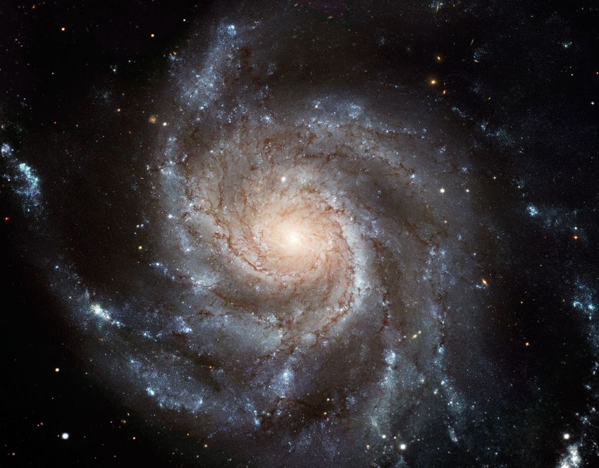
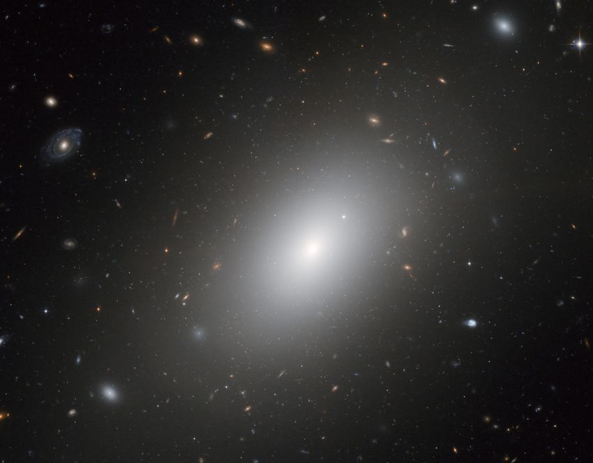
Figure 2.1: An example of two morphology categories: on the left, the spiral
galaxy M101; on the right, the elliptical galaxy NGC 1132 (credit: NASA, ESA,
and the Hubble Heritage Team (STScI/AURA)-ESA/Hubble Collaboration).
learning and image analysis algorithms. But scalability is not the only challenge:
Astronomy applications touch several current machine learning research questions,
such as learning from biased data and dealing with label and measurement noise.
We argue that this makes astronomy a great domain for computer science research,
as it pushes the boundaries of data analysis. In the following, we will present this
exciting application area for data scientists. We will focus on exemplary results,
discuss main challenges, and highlight some recent methodological advancements
in machine learning and image analysis triggered by astronomical applications.
2.2 Ever-Larger Sky Surveys
One of the largest astronomical surveys to date is the Sloan Digital Sky Survey
(SDSS). Each night, the SDSS telescope produces 200 GB of data and now provides
close to a million field images, in which more than 200 million galaxies, and even
more stars, have been detected. A subset of the most visible galaxies formed
the foundation for the crowd-sourced Galaxy Zoo project, in which volunteers
classified more than 900,000 galaxies into one of six morphology categories (see
Figure 2.1). The project was followed by Galaxy Zoo 2, which focused on the
300,000 brightest and largest of the original Galaxy Zoo galaxies [Willett et al.,
2013]. Here, volunteers measured more detailed morphological features of the
galaxies, resulting in 16 million classifications. The images and classifications are
all publicly available, making this a highly valuable dataset for the development
of image analysis and machine learning algorithms.
Upcoming surveys will provide even larger data volumes. Euclid is a space-
based telescope selected by the European Space Agency (ESA) for launch in
2019, which will survey the sky for galaxies and map the large-scale structure
of the Universe. It will generate about 300 GB of image data per night, each
image with a resolution comparable to that of the Hubble Space Telescope. This
will enable precision measurements of the large-scale structure and the expansion
of the Universe, which can help solving some of the hardest and most exciting2.2. Ever-Larger Sky Surveys 15
10 15
10 14 90 TB
Data rate (bytes/night)
30 TB
10 13
10 12
315 GB
200 GB
10 11
10 10 10 GB
VLT SDSS VISTA LSST TMT
(1998) (2000) (2009) (2019) (2022)
Figure 2.2: Increasing data volumes of existing and upcoming telescopes: Very
Large Telescope (VLT), Sloan Digital Sky Survey (SDSS), Visible and Infrared
Telescope for Astronomy (VISTA), Large Synoptic Survey Telescope (LSST) and
Thirty Meter Telescope (TMT).
challenges faced by physicists today, for example explaining dark matter and
dark energy.
Another promising future survey is the Large Synoptic Survey Telescope
(LSST). It will deliver wide-field images of the sky, exposing galaxies that are too
faint to be seen today. One of the main objectives of LSST is to discover transients,
objects that change brightness over time-scales of seconds to months. These
changes are due to a plethora of reasons; some may be regarded as uninteresting
while others will be extremely rare events, which cannot be missed. LSST is
expected to see millions of transients per night, which need to be detected in real-
time to allow for follow-up observations. With staggering 30 TB of images being
produced per night, efficient and accurate detection will be a major challenge.
Figure 2.2 shows how the data rates have increased and will continue to increase as
new surveys are initiated. Future missions will collect hundreds of measurements
for each of more than a billion objects.
What do these measurements look like? Surveys usually take either spectro-
scopic or photometric observations, see Figure 2.3. Spectroscopy measures the
photon count at thousands of wavelengths. The resulting spectrum allows for
identifying the chemical components of the observed object and thus enables
determining many interesting properties. Photometry takes images using a CCD,
and these are typically acquired through only a handful of broad-band filters,
making photometry much less informative than spectroscopy.
While spectroscopy provides measurements of high precision, it has two
drawbacks: First, it is not as sensitive as photometry, meaning that distant or
otherwise faint objects cannot be measured. Second, only few objects can be
captured at the same time, making it more expensive than photometry, which
allows for acquiring images of thousands of objects in a single image. Photometry16 Chapter 2. Machine Learning and Image Analysis for Astronomy
0.5 400
350
0.4
300
Normalized flux
Filter response
0.3 250
200
0.2 150
100
0.1
50
u g r i z
3000 4000 5000 6000 7000 8000 9000 10000 11000
Wavelength (Angstroms)
Figure 2.3: The spectrum of galaxy NGC 5750 (black line), as seen by SDSS,
with the survey’s five photometric broad-band filters u, g, r, i, and z, ranging
from ultraviolet (u) to near-infrared (z ). For each band the galaxy’s brightness
is captured in an image.
can capture objects that may be ten times fainter than what can be measured
with spectroscopy. A faint galaxy is often more distant than a bright one—not
just in space, but also in time. Discovering faint objects therefore offers the
potential of looking further back into the history of the universe, over time-scales
of billions of years. Thus, photometric observations are invaluable to cosmologists,
as they help understanding the early universe.
Once these raw observations have been acquired, a pipeline of algorithms
needs to extract information from them. Much image-based astronomy currently
relies to some extent on visual inspection. A wide range of measurements is still
carried out by humans, but needs to be addressed by automatic image analysis
in light of growing data volumes. Examples are 3D orientation and chirality
of galaxies, and the detection of large-scale features, such as jets and streams.
Challenges in these tasks include image artifacts, spurious effects, and discerning
between merging galaxy pairs and galaxies that happen to overlap along the line
of sight. Current survey pipelines often have trouble correctly identifying these
types of problems, which then propagate into the databases.
A particular challenge is that cosmology relies on scientific analyses of long-
exposure images. As such, the interest in image analysis techniques for prepro-
cessing and de-noising is naturally great. This is particularly important for the
detection of faint objects with very low signal-to-noise ratios. Automatic object
detection is vital to any survey pipeline, with reliability and completeness being
essential metrics. Completeness refers to the amount of detected objects, whereas
reliability measures how many of the detections are actual objects. Maximizing
these metrics requires advanced image analysis and machine learning techniques.
Therefore, data science for astronomy is a quickly evolving field gaining more
and more interest. In the following, we will highlight some of its success stories.2.3. Big Data Analysis in Astronomy 17
2.3 Big Data Analysis in Astronomy
Machine learning methods are able to uncover the relation between input data
(e.g., galaxy images) and outputs (e.g., physical properties of galaxies) based on
input-output samples, and they have already proved successful in astrophysical
contexts. For example, Mortlock et al. [2011] use Bayesian analysis to find the
most distant quasar to date. These are extremely bright objects forming at the
center of large galaxies and thus, are still visible from great distances. They
are, however, also extremely rare. In this case, Bayesian model comparison has
helped the scientists to select a few most likely objects for re-observation from
thousands of plausible candidates.
Another astrophysical application is photometric redshift estimation. Redshift
is caused by the Doppler effect, which shifts the spectrum of an object towards
longer wavelengths when it moves away from the observer. As the universe
is expanding uniformly, we can infer the velocity of a galaxy by its redshift
and, thus, its distance to Earth. Hence, redshift estimation is a useful tool for
determining the geometry of the universe. Redshift can be determined with
high precision by taking a spectroscopic measurement. An important question
in astronomy is, whether it can also be inferred from photometric observations,
since these are easier to acquire. We can build a training set from photometric
measurements whose redshifts are spectroscopically confirmed and subsequently
use, for instance, a neural network to learn a model for predicting the redshifts
[Collister and Lahav, 2004].
With easy access to the publicly available large databases containing data
from astronomical surveys, like SDSS, most big data-oriented work in astronomy
naturally use these as the starting point. Most quantities in these databases are
derived from images taken by the survey telescope(s). The derivation is usually
carried out by the survey consortia, and offered freely to the entire scientific
community with a delay of a year or less. The survey images themselves are,
however, often also freely available online, and offer an enormous potential for
image analysis to enable novel discoveries.
The measurement of galaxy morphologies from images is of major interest
to cosmologists. Morphology can tell astronomers about a galaxy’s formation
and history, which are valuable pieces of information when trying to understand
the Universe as a whole. While the majority of science on galaxy morphology
traditionally involves visual inspection, image analysis algorithms are gaining
momentum. In particular, convolutional neural networks (CNNs) have seen a
growing use in astronomy in the past years. As an example, Galaxy Zoo 2 has
been used to train a CNN to predict galaxy morphologies [Dieleman et al., 2015].
Image analysis is also widely applied in solar physics. The Sun is continuously
being monitored in high resolution by multiple satellites. Image analysis plays a
vital part in detection and classification of both sunspots and the solar eruptions,
such as flares and coronal mass ejections, which they may produce. Eruptions can
have serious consequences for the Earth, as millions of tons of charged particles
are accelerated out from the Sun. An eruption can short-circuit satellites around
the Earth, including the International Space Station, and, if large enough, electric18 Chapter 2. Machine Learning and Image Analysis for Astronomy
systems on the ground. This can knock out power grids for long periods of time,
and especially navigation systems on planes crossing the polar regions are at risk
during high solar activity. Solar eruptions are therefore monitored constantly by
automated software; but not all events are detected [Robbrecht and Berghmans,
2004]. Continuous alert systems using advanced image analysis techniques hold
the potential to increase safety world-wide.
This glimpse of success stories of big data analysis in astronomy is by no
means exhaustive. An overview of machine learning methods that find application
in astronomy can be found in the survey by Ball and Brunner [2010].
2.4 Astronomy Driving Data Science
In the following, we present three examples from our own work showing how
astronomical data analysis can trigger methodological advancements in machine
learning and image analysis.
Describing the Shape of a Galaxy
A galaxy’s morphology is difficult to quantize in a concise manner. It is a
reasonable choice to assign a galaxy a class based on its appearance. Indeed, such
a classification approach has been used since galaxies were first discovered: in a
subjective way by manual inspection. More objective measures of morphology
have been studied, but none have conveyed the same amount of information as
the century-old classification scheme.
Image analysis does not only allow for automatic classification, but can also
inspire new ways to look at morphology [Pedersen et al., 2013, Polsterer et al.,
2015]. For instance, we examined how well one of the most fundamental measures
of galaxy evolution, the star-formation rate, could be predicted from the shape
index. The shape index measures the local structure around a pixel going from
dark blobs over valley-, saddle point- and ridge-like structures to white blobs. It
can thus be used as a measure of the local morphology on a per-pixel scale, see
Figure 2.4. The study showed that the shape index does indeed capture some
fundamental information about galaxies, which is missed by traditional methods.
Dealing with Sample Selection Bias
A challenging theoretical and practical problem in machine learning is caused
by sample selection bias. In supervised machine learning, the models are con-
structed based on labeled examples, that is, observations (e.g., images, spectra,
photometric features) together with their outputs (also referred to as labels, e.g.,
the corresponding redshift or galaxy type). Most machine learning algorithms
are built on the assumption that the training set has been sampled uniformly
at random from the population of interest (i.e., training and future test data
follow the same distribution). This allows for generalization, enabling the model
built from labeled examples in the training set to accurately predict the target
variables in an unlabeled test set. In real-life applications this assumption is2.4. Astronomy Driving Data Science 19
Figure 2.4: From left to right: The original image of a galaxy merger, the
scale-space image of the galaxies, the curvedness (a measure of how pronounced
the local structure is), the shape index, and finally the shape index weighted
by the curvedness. The image shows the Antennae galaxies as seen by the
Hubble Space Telescope (credit: NASA, ESA, and the Hubble Heritage Team
(STScI/AURA)-ESA/Hubble Collaboration).
often violated—we refer to this as sample selection bias. Certain examples are
more likely to be labeled than others due to factors like availability or acquisition
cost regardless of their representation in the population. Sample selection bias
can be very pronounced in astronomical data sets, and machine learning methods
have to address this bias to achieve good generalization.
In astronomy, the mismatch between training and testing data can arise
for several reasons. Often only training data sets from old surveys are initially
available, while upcoming missions will probe never-before-seen regions in the
astrophysical parameter space. Crowd-sourcing efforts like the Galaxy Zoo project
are susceptible to a selection bias, too. As objects have to be recognizable to the
citizen scientists, candidates to be labeled are restricted to a limited depth in
space. Thus, again, certain regions of the input space will be underrepresented
in the training sample.
Fortunately, acquiring large datasets without labels is typically not a problem
anymore. Often we can obtain some labels, for example, by letting an expert
annotate some data or by taking spectroscopic measurements, which are both
costly procedures. This offers a remedy to the sample selection bias problem. We
can either utilize unlabeled examples to improve our model, or we can obtain the
labels of some unlabeled data points. As the latter is costly, we must try to find
the observations that would improve our model the most after labeling.
When the learning algorithm is allowed to choose the examples that maximally
improve the model, we speak of active learning. In the context of sample selection
bias, we can then choose examples that minimize the difference between training
and test distribution. Richards et al. [2012] have demonstrated how active
learning helps to compensate sample selection bias when classifying variable stars
(i.e., different types of stars that change their brightness over time).20 Chapter 2. Machine Learning and Image Analysis for Astronomy
When we do not have the budget or even the possibility to label additional
examples, we can resort to domain adaptation algorithms. These methods assume
that we not only have access to a labeled training set that may be subject to a
selection bias, but also to an unlabeled test set that follows the distribution of the
population, and the latter is used to correct for the bias. Importance-weighting
is a simple, yet effective domain adaptation algorithm. The idea is to give more
weight to examples in the training sample which lie in regions of the feature space
that are underrepresented in the test sample and, likewise, give less weights to
examples whose location in the feature space is overrepresented in the test set. If
these weights are estimated correctly, the model we learn from the training data
is an unbiased estimate of the model we would learn from a sample that follows
the population’s distribution. The challenge lies in estimating these weights
reliably and efficiently. Given a sufficiently large sample, a simple strategy can
be followed: Using a nearest neighbor-based approach, we can count the number
of test examples that fall within a hypersphere whose radius is defined by the
distance to the Kth neighbor of a training example. The weight is then the ratio
of the number of these test examples over K. This flexibly handles regions which
are sparse in the training sample. In the case of redshift estimation, we could
alleviate a selection bias by utilizing a large sample of photometric observations
to determine the weights for the spectroscopically confirmed training set [Kremer
et al., 2015].
Scaling-up Nearest Neighbor Search
Nearest neighbor methods are not only useful to address the sample selection
bias, they have proven to provide excellent prediction results in astrophysics and
cosmology. For example, they are used to generate candidates for quasars at
high redshift [Polsterer et al., 2013]. Nearest neighbor methods work particularly
well when the number of training examples is high and the input space is low-
dimensional. This makes them a good choice for analyzing large sky surveys
where the objects are described by photometric features (e.g., the five intensities
in the frequency bands shown in Figure 2.3). However, searching the nearest
neighbors becomes a computational bottleneck in this big data setting.
In general, powerful compute servers can be employed to reduce the running
time of machine learning algorithms, where the individual nodes conduct parts
of the overall task. However, making use of supercomputers might become
very expensive and parallelizing the work may not be straight-forward. There
are several ways to address this issue, namely the application of special data
structures, the approximation of the underlying problem, or the development of
algorithms that allow for a massively-parallel implementation.
To compute the nearest neighbors for a given query object, spatial search
structures such as k-d trees are an established way to reduce the computational
requirements. If the input space dimensionality is moderate (say, up to 30), the
running time can often be reduced by several orders of magnitude. One could
also apply approximate nearest neighbor search [Arya et al., 1994]. However, we
are interested in the exact solutions for our astronomical data analysis. Thus, we2.4. Astronomy Driving Data Science 21
(host) (host)
top tree
(device)
buffers
(host)
leaf structure
(device)
Figure 2.5: The buffer k-d tree data structure depicts an extension of classical
k-d trees and can be used to efficiently process huge amounts of nearest neighbor
queries using GPUs. The gray components (top tree and leaf structure) are
stored on the device (GPU); the remaining ones (input/reinsert queue and
buffers) are stored on the host CPU system. Nearest neighbor queries are
repeatedly distributed to appropriate leaves and large chunks of queries are
processed together in a massively-parallel manner on the GPU [Gieseke et al.,
2014].
resort to inexpensive massively-parallel devices, graphics processing units (GPUs),
to accelerate the involved computations. Unfortunately, nearest neighbor search
based on spatial data structures cannot be parallelized in an obvious way. To
this end, we developed a new algorithm that allows for efficient massively-parallel
traversal of spatial search structures as sketched in Figure 2.5, which can achieve
a significant running time reduction at a much lower cost compared to traditional
parallel computing architectures. The corresponding framework can be used to
efficiently search for nearest neighbors given large training and test sets with
hundreds of millions of data points [Gieseke et al., 2014]. Such variants of classical
approaches that can handle massive amounts of data efficiently and at low cost
will be crucial for the upcoming data-intensive analyses in astronomy.22 Chapter 2. Machine Learning and Image Analysis for Astronomy
2.5 Physical Models vs. Machine Learning Models
The biggest concern data scientists meet when bringing forward data-driven
machine learning models in astrophysics and cosmology is arguably lack of in-
terpretability. There are two different approaches to predictive modeling in
astronomy: physical modeling and data-driven modeling. The traditional one
is to build physical models, which can incorporate all necessary astrophysical
background knowledge. These models can be used for prediction, for example,
by running Monte Carlo simulations. Ideally, this approach ensures that the
predictions are physically plausible. In contrast, there may be the risk that
extrapolations by a purely data-driven machine learning model violate physical
laws. The decisive feature of physical models is that they also provide an under-
standing of why certain observations could have been made. This interpretability
of predictions is typically not provided when using a machine learning approach.
Physical models have the drawbacks that they are difficult to construct and
that inference may take a long time (e.g., in the case of Monte Carlo simulations).
Most importantly, the quality of the predictions depends on the quality of
the physical model, which is typically limited by necessary simplifications and
incomplete scientific knowledge. In our experience, data-driven models typically
outperform physical models in terms of prediction accuracy [Stensbo-Smidt
et al., 2013, 2015]. Thus, we strongly advocate data-driven models when we
are mainly interested in accurate predictions. And this is indeed often the case,
for example, if we want to estimate properties of objects in the sky for quickly
identifying observations worth a follow-up investigation or for conducting large-
scale statistical analyses. Generic machine learning methods are not meant to
replace physical modeling, because they typically do not provide scientific insights
beyond the predicted values. Still, we argue that if prediction accuracy is what
matters, one should favor the more accurate model, whether it is interpretable or
not. Having said this, while the black-and-white portrayal of the two approaches
may help to illustrate common misunderstandings between data scientists and
physicists, it is of course shortsighted. Physical and machine learning modeling are
not mutually exclusive: Physical models can inform machine learning algorithms,
and machine learning can support physical modeling. A simple example for the
latter is using machine learning to estimate the error residuals of a physical model
[Pedersen et al., 2013].
Dealing with uncertainties is a major issue in astronomical data analysis.
Data scientists are asked to provide error bars for their predictions and have to
think about how to deal with input noise. In astronomy, both input and output
data have (non-Gaussian) errors attached to them. Often these measurement
errors have been quantified (e.g., by incorporating the weather conditions at the
day the data was obtained), and it is desirable to consider these errors in the
prediction. Bayesian modeling and Monte Carlo methods simulating physical
models offer solutions, however, often they do not scale for big data. Alternatively,
one can modify machine learning methods to process error bars, as attempted for
nearest neighbor regression by modifying the distance function [Polsterer et al.,
2013].2.6. A Peek into the Future 23
2.6 A Peek into the Future
The future looks bright for data science in astronomy. Within the next few years,
image analysis and machine learning systems that can process terabytes of data
in near real-time with high accuracy will be essential.
There are great opportunities for making novel discoveries, even in databases
that have been available for decades. The volunteers of Galaxy Zoo have demon-
strated this multiple times by discovering structures in the SDSS images that
have later been confirmed to be new types of objects. These volunteers are not
trained scientists, yet they make new scientific discoveries.
Even today, only a fraction of the images of SDSS have been inspected by
humans. Without doubt, the data still hold many surprises, and upcoming
surveys, such as LSST, are bound to image previously unknown objects. It will
not be possible to manually inspect all images produced by these surveys, making
advanced image analysis and machine learning algorithms of vital importance.
One may use such systems to answer questions like how many types of
galaxies there are, what distinguishes the different classes, whether the current
classification scheme is good enough, and whether there are important sub-classes
or undiscovered classes. These questions require data science knowledge rather
than astrophysical knowledge, yet the discoveries will still help astrophysics
tremendously.
In this new data-rich era, astronomy and computer science can benefit greatly
from each other. There are new problems to be tackled, novel discoveries to be
made, and above all, new knowledge to be gained in both fields.Chapter 3
Active Learning with Support
Vector Machines
This chapter is based on the article J. Kremer, K. Steenstrup Pedersen, and
C. Igel. Active learning with support vector machines. Wiley Interdisciplinary
Reviews. Data Mining and Knowledge Discovery, 4(4):313–326, 2014
Abstract
In machine learning, active learning refers to algorithms that autonomously
select the data points from which they will learn. There are many data
mining applications in which large amounts of unlabeled data are readily
available, but labels (e.g., human annotations or results from complex exper-
iments) are costly to obtain. In such scenarios, an active learning algorithm
aims at identifying data points that, if labeled and used for training, would
most improve the learned model. Labels are then obtained only for the
most promising data points. This speeds up learning and reduces labeling
costs. Support vector machine (SVM) classifiers are particularly well-suited
for active learning due to their convenient mathematical properties. They
perform linear classification, typically in a kernel-induced feature space,
which makes measuring the distance of a data point from the decision
boundary straightforward. Furthermore, heuristics can efficiently estimate
how strongly learning from a data point influences the current model. This
information can be used to actively select training samples. After a brief
introduction to the active learning problem, we discuss different query strate-
gies for selecting informative data points and review how these strategies
give rise to different variants of active learning with SVMs.
3.1 Introduction
In many applications of supervised learning in data mining, huge amounts of
unlabeled data samples are cheaply available while obtaining their labels for
training a classifier is costly. To minimize labeling costs, we want to request labels
only for potentially informative samples. These are usually the ones that we
2526 Chapter 3. Active Learning with Support Vector Machines
expect to improve the accuracy of the classifier to the greatest extent when used
for training. Another consideration is the reduction of training time. Even when
all samples are labeled, we may want to consider only a subset of the available data
because training the classifier of choice using all the data might be computationally
too demanding. Instead of sampling a subset uniformly at random, which is
referred to as passive learning, we would like to select informative samples to
maximize accuracy with less training data. Active learning denotes the process of
autonomously selecting promising data points to learn from. By choosing samples
actively, we introduce a selection bias. This violates the assumption underlying
most learning algorithms that training and test data are identically distributed:
an issue we have to address to avoid detrimental effects on the generalization
performance.
In theory, active learning is possible with any classifier that is capable of passive
learning. This review focuses on the support vector machine (SVM) classifier.
It is a state-of-the-art method, which has proven to give highly accurate results
in the passive learning scenario and which has some favorable properties that
make it especially suitable for active learning: (i) SVMs learn a linear decision
boundary, typically in a kernel-induced feature space. Measuring the distance
of a sample to this boundary is straightforward and provides an estimate of
its informativeness. (ii) Efficient online learning algorithms make it possible to
obtain a sufficiently accurate approximation of the optimal SVM solution without
retraining on the whole dataset. (iii) The SVM can weight the influence of single
samples in a simple manner. This allows for compensating the selection bias that
active learning introduces.
3.2 Active Learning
In the following we focus on supervised learning for classification. There also
exists a body of work on active learning with SVMs in other settings such as
regression [Demir and Bruzzone, 2012] and ranking [Brinker, 2004, Yu, 2005]. A
discussion of these settings is, however, beyond the scope of this article.
The training set is given by L = {(x1 , y1 ), ..., (x` , y` )} ⊂ X × Y. It consists of
` labeled samples that are drawn independently from an unknown distribution
D. This distribution is defined over X × Y, the cross product of a feature space
X and a label space Y, with Y = {−1, 1} in the binary case. We try to infer a
hypothesis f : X → Z mapping inputs to a prediction space Z for predicting the
labels of samples drawn from D. To measure the quality of our prediction, we
define a loss function L : Z × X × Y → R+ . Thus, our learning goal is minimizing
the expected loss h i
R(f ) = E(x,y)∼D L(f (x), x, y) , (3.1)
which is called the risk of f . We call the average loss over a finite sample L the
training error or empirical risk. If a loss function does not depend on the second
argument, we simply omit it.
In sampling-based active learning, there are two scenarios: stream-based
and pool-based. In stream-based active learning, we analyze incoming unlabeled3.3. Support Vector Machine 27
samples sequentially, one sample at a time. Contrary, in pool-based active learning
we have access to a pool of unlabeled samples at once. In this case, we can
rank samples based on a selection criterion and query the most informative ones.
Although, some of the methods in this review are also applicable to stream-based
learning, most of them consider the pool-based scenario. In the case of pool-based
active learning, we have, in addition to the labeled set L, access to a set of m
unlabeled samples U = {x`+1 , ..., x`+m }. We assume that there exists a way to
provide us with a label for any sample from this set (the probability of the label
is given by D conditioned on the sample). This may involve labeling costs, and
the number of queries we are allowed to make may be restricted by a budget.
After labeling a sample, we simply add it to our training set.
In general, we aim at achieving a minimum risk by requesting as few labels
as possible. We can estimate this risk by computing the average error over an
independent test set not used in the training process. Ultimately, we hope to
require less labeled samples for inferring a hypothesis performing as well as a
hypothesis generated by passive learning on L and completely labeled U.
In practice, one can profit from an active learner if only few labeled samples
are available and labeling is costly, or when learning has to be restricted to
a subset of the available data to render the computation feasible. A list of
real-world applications is given in the general active learning survey [Settles,
2012] and in a review paper which considers active learning for natural language
processing [Olsson, 2009].
Active learning can also be employed in the context of transfer learning [Shi
et al., 2008]. In this setting, samples from the unlabeled target domain are
selected for labeling and included in the source domain. A classifier trained on
the augmented source dataset can then exploit the additional samples to increase
its accuracy in the target domain. This technique has been used successfully,
for example, in an astronomy application [Richards et al., 2012] to address a
sample selection bias, which causes source and target probability distributions to
mismatch [Quionero-Candela et al., 2009].
3.3 Support Vector Machine
Support vector machines (SVMs) are state-of-the-art classifiers [Boser et al.,
1992, Cortes and Vapnik, 1995, Mammone et al., 2009, Salcedo-Sanz et al., 2014,
Schölkopf and Smola, 2002, Shawe-Taylor and Cristianini, 2004]. They have
proven to provide well-generalizing solutions in practice and are well understood
theoretically [Steinwart and Christmann, 2008]. The kernel trick [Schölkopf and
Smola, 2002] allows for an easy handling of diverse data representations (e.g.,
biological sequences or multimodal data). Support vector machines perform
linear discrimination in a kernel-induced feature space and are based on the
idea of large margin separation: they try to maximize the distance between the
decision boundary and the correctly classified points closest to this boundary. In
the following, we formalize SVMs to fix our notation, for a detailed introduction
we refer to the recent WIREs articles [Mammone et al., 2009, Salcedo-Sanz et al.,
2014].You can also read