Particles in Loop Quantum Gravity formalism: a thermodynamical description
←
→
Page content transcription
If your browser does not render page correctly, please read the page content below
Particles in Loop Quantum Gravity formalism: a
                                                                          thermodynamical description

                                                                                       A. A. Araújo Filho1, ∗
                                                           1
                                                               Universidade Federal do Ceará (UFC), Departamento de Fı́sica,
                                                           Campus do Pici, Fortaleza - CE, C.P. 6030, 60455-760 - Brazil.
                                                                                       (Dated: March 1, 2022)
arXiv:2202.13907v1 [gr-qc] 28 Feb 2022

                                                                                             Abstract
                                              In this work, we analyse the thermodynamical behavior of massive and massless particles within
                                         Loop Quantum Gravity formalism. We investigate a modified dispersion relation which suffices to
                                         derive all our results of interest in an analytical manner. Initially, we study the massive case where,
                                         in essence, we examine how the mass modifies the thermodynamical properties of the system. On
                                         the other hand, to the massless case, the thermodynamical system turns out to rely only on a
                                         specific thermal state quantity, the temperature. More so, the analysis of the spectral radiation,
                                         the equation of states, the mean energy, the entropy, and the heat capacity are provided as well for
                                         both cases. Finally, the thermodynamical properties of our particles under consideration depends
                                         on the Riemann zeta function ξ(s).

                                         ∗
                                             Electronic address: dilto@fisica.ufc.br

                                                                                                1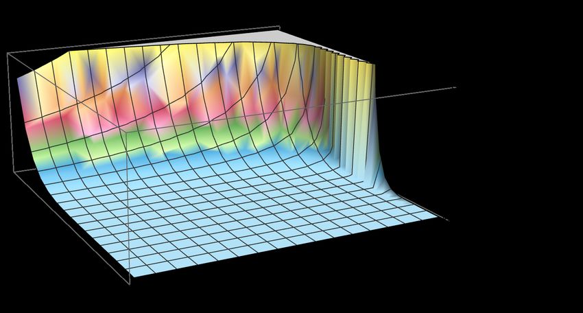
I.    INTRODUCTION

     The insight that the entropy of a black hole should be proportional to its horizon area has
notably contributed to guide quantum gravity research [1–5]. Particularly, in agreement with
Bekenstein [6], the contribution to black hole entropy may be acquired by taking into account
mainly basic elements. Moreover, the correlation involving entropy and event horizon area
established notable constraint in the investigation of quantum gravity formalism.
     Many attempts to reproduce the linearity of the entropy area result utilizing straightfor-
ward quantum properties of black holes failed at the initial stages. Nevertheless, in the last
decades string theory and loop quantum gravity gave rise to some remarkable techniques
that facilitated progress in evaluating entropy when quantum properties of black holes were
considered [7–16]. The essential results are not restricted to the surface area contribution;
they go beyond. Primarily, it is determined that the corrections in the leading order must
be a log-type one. In addition, it is assumed that the relation between the entropy of a black
hole and its respective event horizon takes the form:

                                      A
                                S=       + ρ ln[A/lP2 ] + O(lP2 /A).                        (1)
                                     4lP

     On the other hand, within the context of Loop Quantum Gravity formalism, there does
not exist a consensus on the logarithmic corrections controlled by ρ. Despite this, it is
proposed that the correction terms, superior than the logarithimic dependence on the area,
are absent [10, 11]. In this sense, the comprehension of entropy, i.e., up to the leading log
correction, could be employed to ensure the Planck scale modifications of the components
within the Bekenstein study. It seems to offer a chance to set the viability of working
on some scenarios emerging from Loop Quantum Gravity, e.g., as it is shown in Ref. [5],
where one particular modified dispersion relation is proposed– involving a term with a linear
dependence on the Planck length lP .
     Undoubtedly, a prominent aspect when one deals with a modified dispersion relation is
certainly its respective thermodynamical properties ascribed to a given theory. Investigations
involving thermal aspects in the context of Lorentz violation could supply further knowledge
about primordial stages of expansion of the Universe. In other words, this corroborates the
fact that the size at these stages are consistent with the characteristic scales of Lorentz
violation [17]. The thermal properties within the context of Lorentz symmetry breaking

                                               2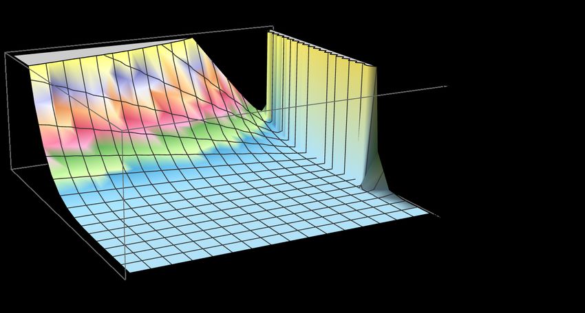
has been initially proposed by Ref. [18]. After that, recently many works have been made
in various distinct scenarios, such as, graviton [19], Pospelov [20] and Myers-Pospelov [21]
electrodynamics, CPT-even and CPT-odd violations [22–24], higher-dimensional operators
[25], bouncing universe [26, 27], and Einstein-eather theory [28].
      Although traditionally many indefinite studies begin with the investigation based on
the action associated with a particular theory, in the literature, there exists a prominent
alternative manner of addressing physical results starting exclusively from its respective
dispersion relation instead [29]. Also, in this context, there are a lack of studies examining
the thermodynamic properties in the context of Loop Quantum Gravity up to now. In
this sense, we follow the methodology developed in Ref. [18] in order to accomplish a
thermodynamic description of the system. We take into account two kinds of particles: the
massive and the massless ones. For all of them, we perform the analysis of the following
respective state thermodynamic physical quantities: the equation of states, the mean energy,
the spectral radiance, the entropy, and the heat capacity.

II.     THE MASSIVE CASE

      The possibility of Planck-scale modifications of the dispersion relation has been exten-
sively considered in the quantum gravity literature [30–45] and, specifically, in Loop Quan-
tum Gravity scenario [46–53]. Although customarily many examinations begin theirs in-
vestigations with the action associated with a particular theory, there exists a prominent
alternative manner in the literature of addressing physical results from its dispersion relation
only [29]. Here, such procedure is invoked seeking to provide the development of the ther-
modynamic properties. This section is devoted to study massive particles within the context
of Loop Quantum Gravity formalism proposed by Ref. [5]. In this one, based on the black
hole area-entropy law, it is proposed several constraints concerning Loop Quantum Grav-
ity energy-momentum dispersion relation. Likewise, we start with the following dispersion
relation in order to develop a procedure to acquire the thermodynamic state functions:

                                              m2
                                     E 'k+       + αlP E 2 ,                                (2)
                                              2k

where, E is the energy, k is the momentum, m is the mass, α is an arbitrary constant, and
     √
lP = 8πG. Notice that the relation between energy and momentum has a different form

                                              3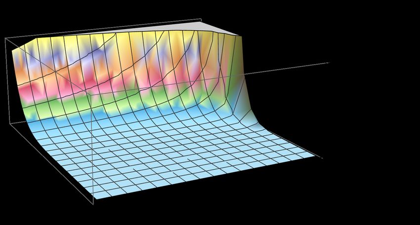
from the usual one, as we could naturally expect. In other words, this aspect indicates that
the Lorentz symmetry is no longer preserved [54, 55] in such a context. Moreover, from the
above expression, we can clearly obtain two solutions; nevertheless, accomplishing a Wick-
like rotation in the mass term, only one of them is in agreement with our purpose, i.e., of
having a real positive definite values, which is
                            1     p
                      k=       2E + (2E − 2E 2 lP ) 2 + 8m2 − 2E 2 lP ,                         (3)
                            4
where we have considered α = 1, and, naturally, we can derive its infinitesimal quantity dk
as follows:                                                                        !
                                                                2
                            1   (2 − 4ElP ) (2E − 2E lP )
                     dk =       p                          − 4ElP + 2 dE.                       (4)
                            4      (2E − 2E 2 lP ) 2 + 8m2
With these above expressions, we are able to perform the integration over the momenta
space in order to acquire the accessible states of the system
                                               ˆ
                                            Γ ∞
                                   Ω(E) = 2         dk|k|2 ,                                    (5)
                                            π 0
where Γ is regarded as the volume of the thermal reservoir. Thereby, Eq. (5) reads
                          ˆ                                              !
                        Γ ∞ 1 (2 − 4ElP ) (2E − 2E 2 lP )
                Ω(E) = 2            p                         − 4ElP + 2
                        π 0 64        (2E − 2E 2 lP ) 2 + 8m2                                   (6)
                               p                                 2
                        × 2E + (2E − 2E 2 lP ) 2 + 8m2 − 2E 2 lP dE.

It is worthy to be mentioned that all calculation present in this manuscript will be ac-
complished in a “per volume” approach. Seeking a better comprehension to the reader, we
provide the most general definition of the partition function considering an indistinguishable
spinless gas [56]:
                                       ˆ                                    ˆ
                                 1                        3N −βH(q,p)
                Z(T, Γ, N ) =              dq   3N
                                                     dp     e           ≡       dE Ω(E)e−βE ,   (7)
                              N !h3N
where, here, we have h being the Planck’s constant, H being the Hamiltonian of the system,
p being the generalized momenta, q being the generalized coordinates, and N being the
number of particles. However, notice that Eq. (7) does not suffice to categorize the spin
of the respective particles under consideration. For our study, such a feature has to be
implemented in the following manner [57–61]
                                    ˆ
                             ln[Z] = dE Ω(E)ln[1 − e−βE ],                                      (8)

                                                     4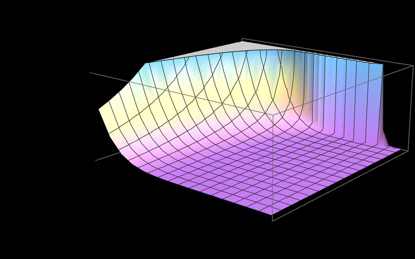
where the factor ln[1 − e−βE ] accounts for the Bose-Einstein statistics. Thereby, we are able
to derive the partition function in a straightforward way:
                           ˆ                                               !
                        Γ ∞ 1 (2 − 4ElP ) (2E − 2E 2 lP )
   ln[Z(lP , m, β)] = − 2            p                          − 4ElP + 2
                        π 0 64          (2E − 2E 2 lP ) 2 + 8m2                             (9)
                                 p                                 2
                        × 2E + (2E − 2E 2 lP ) 2 + 8m2 − 2E 2 lP ln(1 − e−βE ) dE.
In possession with above expression, we are capable of inferring all thermal quantities of
interest that we shall investigate in the following sections. As we shall see, in their totally,
the expressions are much complicated to be solved in an analytical way, i.e., they have
numerical solutions only. However, under a certain limit, they can properly be provided in
an exact form. The definitions of the thermodynamic functions are given by
                                           1
                             F (β, m) = − ln [Z(β, m)] ,
                                           β
                                            ∂
                             U (β, m) = − ln [Z(β, m)] ,
                                           ∂β
                                                                                           (10)
                                               ∂
                             S(β, m) = kB β 2 F (β, m),
                                              ∂β
                                                  ∂
                             CV (β, m) = −kB β 2 U (β, m),
                                                 ∂β
where F (β, m) is the Helmholtz free energy, U (β, m) is the mean energy, S(β, m) is the
entropy, and CV (β, m) is the heat capacity. Furthermore, at the begging, we initiate with the
examination of the equation of states of the system, which is present in the next subsection.

   A.    Equation of states

   This subsection is devoted to explore the consequences of the equation of states of a
system composed exclusively by massive particles; to step toward to the calculation, we
write:
                                         dF = −S dT − p dV,                                (11)

which, straightforwardly, it gives rise to

                                       ˆ ∞                                          !
                                           1 (2 − 4ElP ) (2E − 2E 2 lP )

                        ∂F         1
 p(lP , m, β) = −                = 2         p                           − 4ElP + 2
                        ∂V   T    βπ 0 64       (2E − 2E 2 lP ) 2 + 8m2
                                          p                                2
                                  × 2E + (2E − 2E 2 lP ) 2 + 8m2 − 2E 2 lP ln(1 − e−βE ) dE.
                                                                                           (12)

                                                 5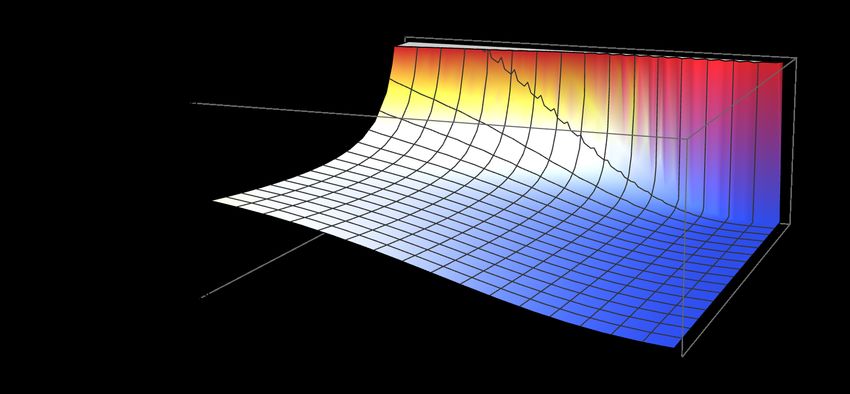
Since there is no exact solution to the above expression, we shall consider the limit where
(2E − 2E 2 lP ) 2
1. The usage of this limit is totally reasonable since parameters which
control the Lorentz symmetry breaking are expect to be very small [17]. With it, we obtain
an analytical solution to Eq. (12) as follows
1 h √ √
2 2 6 2 2
p(lP , m, β) = √ 2
60β lP 2π β m + 189 2 β m ζ(5) + 15ζ(7)
2520 m2 β 9
√ √ √
−β 3 lP 63π 4 2β 2 m2 + 1260β m2 β 2 m2 ζ(3) + 18ζ(5) + 20π 6 2
√ (13)
√ √
−84βlP3 2700β m2 ζ(7) + π 8 2 + 1587600 2ζ(9)lP4
√ √ i
4 2 3 2 3/2 4 2 2
+21β 5π β m 2
+ π β m + 45 2 β m ζ(3) + ζ(5) ,
where ζ(s) is the Riemann zeta function given by
∞ ˆ ∞ s−1 ˆ ∞
X 1 1 x
ζ(s) = s
= dx, Γ(s) = xs−1 e−x dx. (14)
n=1
n Γ(s) 0 ex − 1 0
In order to provide a concise analysis to this thermodynamic property, we supply its re-
spective plot. The initial consideration presented here is that the temperature is fixed while
there exists a change in the mass of the system; such behavior is shown in Fig. 1. Notice
that the system is sensitive to the change of mass, i.e., being more accentuated for higher
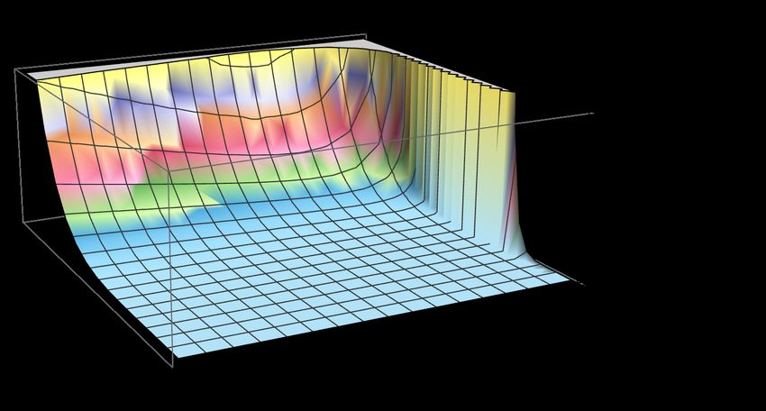
values of m. On the other hand, if we regard fixed values of m while the temperature varies,
we will acquire the behavior exhibited in Fig. 2. In this case, up to very low temperatures
though, there is no much change in the shape of the plot ascribed to the modification of the
temperature.
B. The mean energy
Here, we present the main features ascribed to the mean energy concerning the massive
particles. The calculation of this quantity is so important, among other features, because one
can correlate, for instance, the work felt by the system with the total amount of heat within
it. In other words, with it, we can infer about the well-known first law of thermodynamics.
Moreover, another interesting facet to this thermal quantity is the obtainment of the spectral
6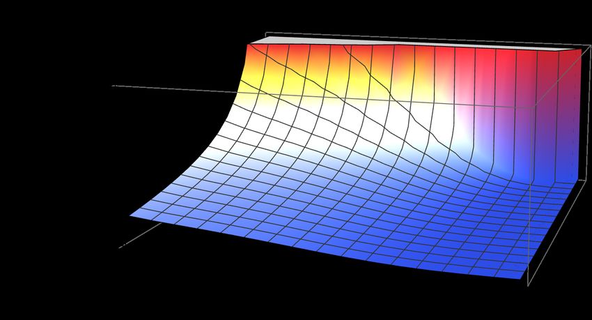
Figure 1: The equation of states for different values of mass keeping the same magnitude of
temperature.

radiance directly from its integrating. To proceed these calculations, we write
                         ˆ ∞                                            !
                              E (2 − 4ElP ) (2E − 2E 2 lP )
         U (lP , m, β) =           p                         − 4ElP + 2
                          0  64      (2E − 2E 2 lP ) 2 + 8m2
                                                                                       (15)
                               p                                2    e−βE
                          2E + (2E − 2E 2 lP ) 2 + 8m2 − 2E 2 lP                dE.
                                                                    (1 − e−βE )
Analogously to what we have carried out to the equation of states, the limit
(2E − 2E 2 lP ) 2  1 is also considered. After this consideration, the mean energy is cal-
culated in an analytical way:
                     1         √        √ h          √ √
U (lP , m, β) =         √       −4 m2 − 2 126β 2 lP π 4 2β m2 + 20β 2 m2 ζ(3) + 240ζ(5)
                10080β 7 m2
                         √ √
                −40βlP 756 2β m ζ(5) + 5π + 453600ζ(7)lP3
                      2               2       6

                                      √ √              i
                −21β 3 5π 2 β 2 m2 + 60 2β m2 ζ(3) + π 4 .
                                                                                       (16)

We devote our attention to perform the verification of how mass changes the mean energy;
such analysis is displayed in Fig. 3. From it, we realize that there is no significant modi-

                                            7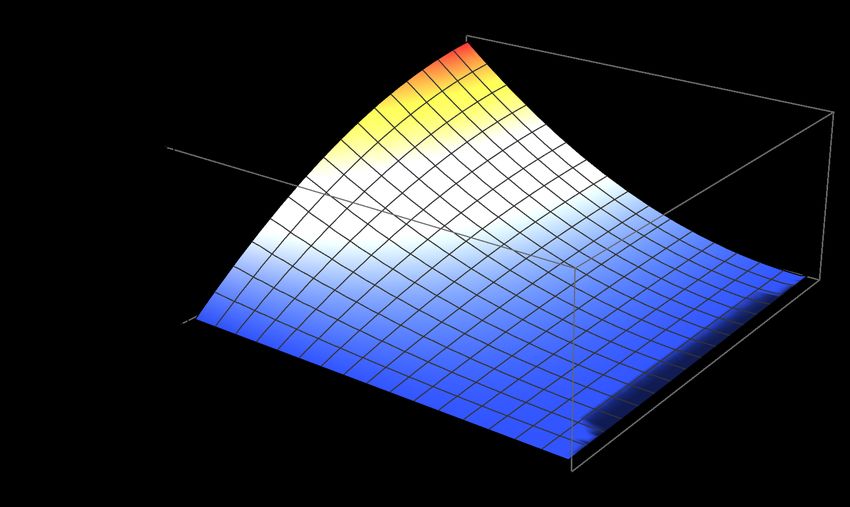
Figure 2: The equation of states for different values of temperature keeping the same magnitude
of mass.

fications in the shape of the plot to diverse values of mass keeping the same temperature.
Furthermore, the behavior of the system for distinct magnitudes of temperatures is another
topic worth exploring. In contrast, when we consider the change of the values of temperature
maintaining the magnitude of mass constant, we have Fig. 4. In this configuration of the
system, we clearly see that if the range of temperature is T ≤ 1 GeV, the system indicates
instability.

   C.      The spectral radiance

   The spectral radiance is given by
                                                                       !
                        hν (2 − 4hνlP ) (2hν − 2(hν)2 lP )
           χ(m, β, ν) =       p                            − 4hνlP + 2
                        64     (2hν − 2(hν)2 lP ) 2 + 8m2
                                                                                             (17)
                              p                                       2      e−βhν
                          2hν + (2hν − 2(hν)2 lP ) 2 + 8m2 − 2(hν)2 lP                   ,
                                                                            (1 − e−βhν )

                                              8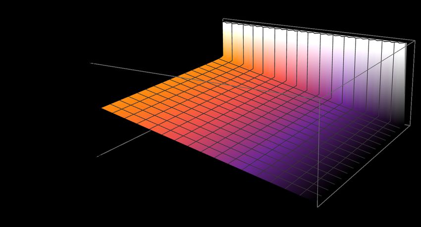
Figure 3: The mean energy for different values of mass maintaining the same magnitude of tem-
perature

where we have considered E = hν, with ν being the frequency. The behavior of the well-
known spectral radiance is exhibited in Fig. 5 for three different regimes of temperature of
the universe, e.g., T = 1013 GeV (inflationary era), T = 103 GeV (electroweak epoch), and
T = 10−13 GeV (cosmic microwave background). Note that the first two sets of temperature
show a perfect shape of the black body radiation up to a sing; nevertheless, to these cases,
the system also indicates instability, as one could naturally expect from the results derived
in the last subsection. On the other hand, the last configuration indicates that the shape of
the plot is close to that one shown in the Wien’s energy density distribution instead. The
next thermodynamic function worth studying is the entropy. To provide such an analysis,
we devote the next subsection to it.

  D.       Entropy

  The necessity of having information about the entropy encountered in the system precedes
itself. The knowledge of such thermal quantity is notable since we are certainly able to

                                            9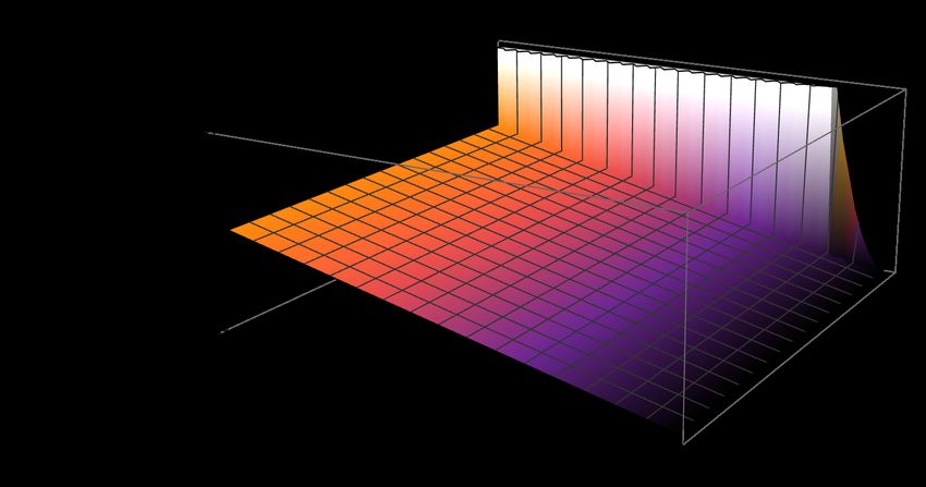
Figure 4: The mean energy for different values of temperature maintaining the same magnitude of
mass
address the behavior of the constituents of matter in a proper manner– the second law of
thermodynamics. In this sense, the entropy is written as
(2−4ElP )(2E−2E 2 lP )
ˆ ∞ ln 1 − e−βE √ − 4ElP + 2
1 (2E−2E 2 lP )2 +8m2
S(lP , m, β) = − 2
0 β 64β 2
p
2E + (2E − 2E 2 lP ) 2 + 8m2 − 2E 2 lP 2
×
64β 2 (18)
(2−4ElP )(2E−2E 2 lP )
Ee−βE √ − 4ElP + 2
(2E−2E 2 lP )2 +8m2
−
64β (1 − e−βE )
p
2E + (2E − 2E 2 lP ) 2 + 8m2 − 2E 2 lP 2
× dE.
64β (1 − e−βE )
It is important to mention that above expression does not possess an analytical solution. In
order to carry out this integral in an exact way, we use the limit where (2E − 2E 2 lP ) 2
1.
100 0
13 27
T = 10 GeV -5.0 × 10 T = 103 GeV
39
-5.0 × 10 -1.0 × 1028
m=1x10¹⁰ GeV -1.5 × 1028 m=1x10¹⁰ GeV
χ(ν)
χ(ν)
40
-1.0 × 10 -2.0 × 1028
m=2x10¹⁰ GeV m=2x10¹⁰ GeV
m=3x10¹⁰ GeV -2.5 × 1028
m=3x10¹⁰ GeV
-1.5 × 1040
-3.0 × 1028
m=4x10¹⁰ GeV m=4x10¹⁰ GeV
0 100 000 200 000 300 000 400 000 500 000 0 2000 4000 6000 8000 10 000
ν ν
5 × 10⁸
T = 10-13 GeV
4 × 10⁸
3 × 10⁸ m=1x10¹⁰ GeV
χ(ν)
m=2x10¹⁰ GeV
2 × 10⁸
m=3x10¹⁰ GeV
1 × 10⁸
m=4x10¹⁰ GeV
0
2. × 10-13 4. × 10-13 6. × 10-13 8. × 10-13 1. × 10-12
ν
Figure 5: The spectral radiance for the massive case
With this assumption, we get
√ √ √ √ √
−4βlP 45β m2 ζ(3) + π 4 2 + 900 2ζ(5)lP2 + 5β 2 2π 2 β m2 + 9 2ζ(3)
S(lP , m, β) = √ .
960β 4 m2
(19)
With the purpose of verifying how this thermodynamic function behaves in terms of m, and
T , we provide a plot which is displayed in Fig. 6. Here, the mass is kept constant while
we vary the temperature. The system turns out to be sensitive to the change of the values
of temperature in a prominent manner. More so, it is worthy to be noted that when the
temperature lies between the range of 0 ≤ T ≤ 1 – whenever m = 103 GeV –, the system
seems to possess instability. On the other hand, another interesting aspect naturally arises:
what would be the comportment of the entropy if different values of mass were taken into
account? To answer this question, we properly provide Fig. 7. Again, the system is quite
sensitive to the modification of mass. Note that it tends to have a shape in the form of a
sheet for huge values of m.
11Figure 6: The entropy for the massive case when the mass is kept the same
E. The heat capacity
Being an inherent property of any arbitrary substance, the heat capacity is, summarily,
the amount of heat energy required to raise its temperature by one unit. Thereby, it is
worth knowing such aspect in the context of massive particles in order to have a better
comprehension of how mass affects such a system. Then, the heat capacity is given by
(2−4El )( 2E−2E 2l
)
ˆ ∞ 2 −βE P P
√ − 4ElP + 2
E e
2
(2E−2E 2 lP )2 +8m2
CV = β
0 64 (1 − e−βE )
p
2E + (2E − 2E lP ) + 8m − 2E lP 2
2 2 2 2
×−
64 (1 − e−βE ) (20)
(2−4ElP )(2E−2E 2 lP )
E 2 e−2βE √ 2 2 2
− 4ElP + 2
(2E−2E lP ) +8m
64 (1 − e−βE )2
p
2E + (2E − 2E 2 lP ) 2 + 8m2 − 2E 2 lP 2
×− dE.
64 (1 − e−βE )2
12Figure 7: The entropy for the massive case when the temperature is kept the same
Here, the same fact occurred to this thermal function: there is no analytical solution. How-
ever, after applying the limit (2E − 2E 2 lP ) 2
1, we obtain
1 h √ √
CV = √ 300β 2 lP2 2π 6 β m2 + 63 2 2β 2 m2 ζ(5) + 63ζ(7)
420β 8 m2
√ √ √
−2β 3 lP 63π 4 2β 2 m2 + 630β m2 β 2 m2 ζ(3) + 60ζ(5) + 50π 6 2
√ (21)
√ √
−784βlP 2025β m ζ(7) + π 2 + 19051200 2ζ(9)lP4
3 2 8
3/2 √ √ i
+7β 4 5π 2 β 3 m2 + 6π 4 β m2 + 45 2 3β 2 m2 ζ(3) + 10ζ(5) .
Analogously to we did to the previous thermodynamic state quantities, initially, we provide
an analysis based on fixed values of mass. Such behavior is shown in Fig. 8. The intriguing
features here is that when the temperature lies in 0 < T < 6 GeV, the system brings out
instability. On the other hand, when the temperature is kept constant, we have the behavior
shown in Fig. 9. In this case, the mass also plays an important role in this thermodynamical
property of our system under consideration.
13Figure 8: The heat capacity for different values of temperature while the mass is maintained
constant
III. THE MASSLESS CASE
In this section, we focus exclusively on the features ascribed to the massless case. As we
did before, the same procedure will be implemented here. In other words, we seek for the
accessible state of the system in order to build up the partition function of our ensemble of
particles. In this sense, using the same dispersion relation pointed out previously,
m2
E 'k+ + αlP E 2 ,
2k
we may consider the case where m → 0. Thereby, the dispersion relation related to the
massless case is obtained in a straightforward manner:
E ' k + αlP E 2 . (22)
With this, the accessible states can be derived after integrating over the momentum space
as follows ˆ ∞ 2
Ω2 (E) = (1 − 2ElP ) E − E 2 lP dE. (23)
0
14Figure 9: The heat capacity for different values of mass while the temperature is maintained
constant
In possession of this quantity, the obtainment of the partition function turns out be a
straightforward task
ˆ ∞ 2
(1 − 2ElP ) E − E 2 lP ln 1 − e−βE dE.
ln[Z2 (β)] = − (24)
0
As it is well-known from the literature, after knowing the partition function, we are properly
able to address the complete behavior of our thermal system and, therefore, all the thermo-
dynamic functions may be obtained. Likewise, in this section, we provide the same thermal
quantities calculated to the massive case, i.e., the equation of states, the spectral radiance,
the entropy, and the heat capacity. Notably, without any particular limit, the results to
this case are carried out in an analytical way. It is worth mentioning that analytical results
involving higher Lorentz-violating scenarios are quite rare even in the context of certain
specific approximations. Furthermore, in order to continue our investigation, we initially
start with the equation of states.
15A. Equation of states
When one desires to know about the main aspects of given specific thermodynamical
system under consideration, inevitably, one stumbles upon the study of the equation of
states. Fundamentally, this occurs because it relates some physical state quantities, such as,
pressure, temperature, and volume. Nevertheless, as we shall see, concerning the massless
case, the main features is that it correlates the main thermodynamical functions with the
temperature and the Riemann zeta function. In this way, we have
ˆ ∞
2
(1 − 2ElP ) E − E 2 lP ln 1 − e−βE dE,
p2 = (25)
0
which results
−7π 4 T 3 + 75600lP3 ζ(7) − 40π 6 T 5 lP2 + 7560T 4 lP ζ(5)
p2 (T ) = . (26)
315
Clearly, we see that the pressure has its dependency concerning only on two variables: the
temperature T , and the Riemann zeta function ξ(s). For the sake of a better comprehension
to the reader, we plot the equation of states in Fig. 10. Note that there exists a huge
1.5 × 1080
1.0 × 1080
p 2 (T)
5.0 × 1079
0
0 2 × 10¹² 4 × 10¹² 6 × 10¹² 8 × 10¹² 1 × 10¹³
T
Figure 10: The equation of states for different values of temperature.
increment of pressure for different values of temperature. Thereby, the system under con-
sideration, i.e., without mass, up to some specific sets, indicates stability since the results
are agreement with the literature– the second law of the thermodynamics is maintained.
Another remarkable information to know about our system is, undeniably, the verification
of how the mean energy behaves when mass is no longer invoked.
16B. The mean energy
In order to provided a better comprehension of the thermodynamical aspects in our
investigation, specially, to infer about the amount of work and heat exchanged by the system,
it is resealable to have the knowledge of the mean energy. In other words, in possession with
it, the first law of the thermodynamics can naturally be addressed. In this sense, we proceed
forward writing the proper expression to the mean energy as follows:
ˆ ∞ 2
Ee−βE (1 − 2ElP ) (E − E 2 lP )
U2 = dE, (27)
0 1 − e−βE
where, after evaluating above expression, we obtain
π4T 4 40π 6 lP2 T 6
U2 (T ) = − 1440lP3 ζ(7)T 7 + − 96lP ζ(5)T 5 . (28)
15 63
For the sake of elucidating the comportment of this quantity, we provide the plot shown in
6. × 10-52
5. × 10-52
4. × 10-52
U2 (T)
3. × 10-52
2. × 10-52
1. × 10-52
0
0 2. × 10-14 4. × 10-14 6. × 10-14 8. × 10-14 1. × 10-13
T
Figure 11: The mean energy for different values of temperature.
Fig. 11. Here, we clearly see that the first law and the second law of thermodynamics are
preserved considering this simpler case, the massless case. Moreover, there exists another
important feature that may be derived from the knowledge of the mean energy, the spectral
radiance. Thereby, we examine this physical quantity in the next subsection.
17C. The spectral radiance
Here, we supply the study of the black body radiation which is written as
2
hνe−βhν (1 − 2hνlP ) (hν − (hν)2 lP )
χ2 (β, ν) = . (29)
1 − e−βhν
Notice that, to this present massless case, the same feature encountered in the massive case
remains: the possibility of instabilities when either the electroweak epoch (T = 103 GeV)
or the inflationary era (T = 1013 GeV) regime of temperature of the universe are taken into
account. Remarkably, the stability gives rise to when the cosmic microwave background
regime of temperature (T = 10−13 GeV) is considered instead. A detailed representation of
these particularities of the spectral radiance is exhibited in Fig. 12.
0 0
3
T = 10 GeV T = 1013 GeV
-5.0 × 10¹⁹
-2 × 1079
-1.0 × 10²⁰ m=1.0x10¹⁰ GeV m=1.0x10¹³ GeV
χ 2 (ν)
χ 2 (ν)
79
-4 × 10
m=1.1x10¹⁰ GeV m=1.1x10¹³ GeV
-1.5 × 10²⁰
m=1.2x10¹⁰ GeV -6 × 1079 m=1.2x10¹³ GeV
-2.0 × 10²⁰
m=1.3x10¹⁰ GeV m=1.3x10¹³ GeV
0 5000 10 000 15 000 20 000 0 1 × 10¹⁴ 2 × 10¹⁴ 3 × 10¹⁴ 4 × 10¹⁴
ν ν
-39
1.4 × 10 m=1.0x10⁻¹³ GeV
1.2 × 10-39
m=1.1x10⁻¹³ GeV
1. × 10-39
m=1.2x10⁻¹³ GeV
8. × 10-40
χ 2 (ν)
6. × 10-40 m=1.3x10⁻¹³ GeV
4. × 10-40
2. × 10-40
0 T = 10-13 GeV
0 2. × 10-13 4. × 10-13 6. × 10-13 8. × 10-13 1. × 10-12
ν
Figure 12: The spectral radiance for the massless case
D. Entropy
One of the main concerns of knowing this thermodynamical state quantity is ensuring
weather the process of reversibility is present in our system or not. In other words, such
18information lies in the core of the second law of the thermodynamics. In this way, in order
to provide such an analysis, we write the entropy to the massless case as
ˆ ∞ 2 2 −βE
−βE 2 2
!
(1 − 2ElP ) (E − E lP ) ln 1 − e Ee (1 − 2ElP ) (E − E lP )
S2 = −β 2 − dE.
0 β 2 β (1 − e−βE )
(30)
Notice that this integral can be evaluated without considering any particular limit. There-
fore, we have
4 (7π 4 T 3 + 60π 6 lP2 T 6 − 9450T 4 lP ζ(5))
S2 (T ) = − 1680lP3 ζ(7)T 6 . (31)
315
Its whole behavior as a function of temperature is exhibited in Fig. 13. Again, in this case,
there exists an accentuated augmentation in the entropy for different values of temperature.
Finally, to complete our analysis, we have to study the comportment of the heat capacity.
To do this, we devote the next subsection for the sake of showing the main characteristics
to this remaining quantity.
8. × 10-39
6. × 10-39
S2 (T)
4. × 10-39
2. × 10-39
0
0 2. × 10-14 4. × 10-14 6. × 10-14 8. × 10-14 1. × 10-13
T
Figure 13: The entropy for different values of temperature.
E. The heat capacity
For finishing our investigation concerning the thermodynamical properties of the massless
case, we present the heat capacity
ˆ ∞ 2 −βE 2 2 2 −2βE 2 2
!
E e (1 − 2El P ) (E − E lP ) E e (1 − 2El P ) (E − E lP )
C2V = −β 2 − − dE.
0 1 − e−βE (1 − e−βE )2
(32)
19Analogously to all thermal quantities calculated up to now considering the massless sector,
this one has also an analytical solution:
4 (−7π 4 T 3 + 264600lP3 ζ(7)T 6 − 100π 6 T 5 lP2 + 12600T 4 lP ζ(5))
C2V (T ) = − . (33)
105
More so, its behavior is shown in Fig. 14. Likewise, there is an accentuated increase of its
respective curve representing the heat capacity when the temperature increases.
2.5 × 10-38
2. × 10-38
C2 V (T)
1.5 × 10-38
1. × 10-38
5. × 10-39
0
0 2. × 10-144. × 10-146. × 10-148. × 10-141. × 10-13
T
Figure 14: The heat capacity for different values of temperature.
Summarily, as we could verified through the manuscript, the main feature for this simplest
massless case is that all the thermal properties follow a similar behavior, i.e., the manner
that the plot increases as a function of the temperature T only.
IV. CONCLUSION
This work was aimed at analysing the thermodynamical behavior of massive as well as
massless particles within the context of Loop Quantum Gravity approach. It was considered
a modified dispersion relation which was sufficient to derive all our results in an analytical
way. At the beginning, we investigated the massive case where, fundamentally, we verified
how the mass modified the thermodynamical functions of the system. On the other hand,
in the massless case, the thermodynamical system turned out to depend only on a specific
thermal state quantity, the temperature. Furthermore, the examination of the spectral
radiation, the equation of states, the mean energy, the entropy and the heat capacity were
also accomplished for both cases. Additionally, the thermodynamical properties of our
20particles under consideration had an explicit dependence on the Riemann zeta function
ξ(s).
Within the context of the equation of states, we noticed that, for the massive case, the
system was sensitive to the changes of mass. Similarly, in the massless case, we observed
that there existed a huge increment of pressure for different values of temperature. Then,
the system under consideration, up to some specific sets, indicated stability since the results
were in agreement with the literature– the second law of thermodynamics was maintained.
Concerning the mean energy, we comprehended that there was no substantial modifica-
tions in the form of the graphics for different values of mass maintaining a fixed value of
temperature. Conversely, when we observed the change of the values of temperature while
maintaining constant the magnitude of mass, we clearly perceived that if the range of tem-
perature was T ≤ 1 GeV, the system would indicate instability. More so, to the massless
case, the mean energy had a huge increase in distinct values of temperature.
The spectral radiation to the massive case where performed within the context of three
distinct regimes of temperature, i.e., inflationary era (T = 1013 GeV), electroweak epoch
(T = 103 GeV), and the cosmic microwave background (T = 10−13 GeV). In the config-
uration presented in the first two ones, our results suggested an existence of instability.
Nevertheless, only in the latter scenario, the system had a perfect shape of black body ra-
diation. On the other hand, to the massless case, the same regime of temperature was also
taken into account. Within the inflationary era (T = 1013 GeV) and the electroweak epoch
(T = 103 GeV), the system seemed to indicate instability. Irrespective of this, when the
cosmic microwave background scheme of temperature (10−13 GeV) was invoked, we had the
shape of the Wien’s energy density distribution instead.
In the context of the entropy, the system turned out to be responsive to the changes
of the values of temperature in a recognizable manner. Furthermore, it was noted if the
temperature lied in the range 0 ≤ T ≤ 1, i.e., with m = 103 GeV, the system would
possess instability. On the other hand, to the massless case, there existed an accentuated
augmentation in the entropy behavior for distinct values of temperature.
Finally, to the heat capacity, some intriguing features emerged. For instance, when the
temperature lied in 0 < T < 6 GeV, the system showed instability. And, considering
the massless case instead, the heat capacity increased in a huge way when there was a
modification in the temperature.
21Acknowledgments
This work has been supported by Conselho Nacional de Desenvolvimento Cientı́fico e
Tecnológico (CNPq) - 142412/2018-0. Most of the calculations presented in this manuscript
were accomplished by using the Mathematica software. More so, we would like to thank
Izeldin and Mylkleany for the careful reading of this manuscript.
[1] C. Rovelli, Quantum gravity. Cambridge university press, 2004.
[2] C. Kiefer, “Why quantum gravity?,” in Approaches to fundamental physics, pp. 123–130,
Springer, 2007.
[3] E. Bianchi, P. Dona, and S. Speziale, “Polyhedra in loop quantum gravity,” Physical Review
D, vol. 83, no. 4, p. 044035, 2011.
[4] S. Carlip, “Quantum gravity: a progress report,” Reports on progress in physics, vol. 64, no. 8,
p. 885, 2001.
[5] G. Amelino-Camelia, M. Arzano, and A. Procaccini, “Severe constraints on the loop-quantum-
gravity energy-momentum dispersion relation from the black-hole area-entropy law,” Physical
Review D, vol. 70, no. 10, p. 107501, 2004.
[6] J. D. Bekenstein, “Black holes and entropy,” in JACOB BEKENSTEIN: The Conservative
Revolutionary, pp. 307–320, World Scientific, 2020.
[7] A. Ghosh, K. Noui, and A. Perez, “Statistics, holography, and black hole entropy in loop
quantum gravity,” Physical Review D, vol. 89, no. 8, p. 084069, 2014.
[8] R. Mansuroglu and H. Sahlmann, “Fermion spins in loop quantum gravity,” Physical Review
D, vol. 103, no. 6, p. 066016, 2021.
[9] Y. Xiao and Y. Tian, “Logarithmic correction to black hole entropy from the nonlocality of
quantum gravity,” Physical Review D, vol. 105, no. 4, p. 044013, 2022.
[10] C. Rovelli, “Black hole entropy from loop quantum gravity,” Physical Review Letters, vol. 77,
no. 16, p. 3288, 1996.
[11] A. Ashtekar, J. Baez, A. Corichi, and K. Krasnov, “Quantum geometry and black hole en-
tropy,” Physical Review Letters, vol. 80, no. 5, p. 904, 1998.
[12] R. K. Kaul and P. Majumdar, “Logarithmic correction to the bekenstein-hawking entropy,”
22Physical Review Letters, vol. 84, no. 23, p. 5255, 2000.
[13] A. Strominger and C. Vafa, “Microscopic origin of the bekenstein-hawking entropy,” Physics
Letters B, vol. 379, no. 1-4, pp. 99–104, 1996.
[14] S. N. Solodukhin, “Entropy of the schwarzschild black hole and the string–black-hole corre-
spondence,” Physical Review D, vol. 57, no. 4, p. 2410, 1998.
[15] S. N. Solodukhin, “Logarithmic terms in entropy of schwarzschild black holes in higher loops,”
Physics Letters B, vol. 802, p. 135235, 2020.
[16] K. A. Meissner, “Black-hole entropy in loop quantum gravity,” Classical and Quantum Gravity,
vol. 21, no. 22, p. 5245, 2004.
[17] V. A. Kosteleckỳ and N. Russell, “Data tables for lorentz and c p t violation,” Reviews of
Modern Physics, vol. 83, no. 1, p. 11, 2011.
[18] D. Colladay and P. McDonald, “Statistical mechanics and lorentz violation,” Physical Review
D, vol. 70, no. 12, p. 125007, 2004.
[19] A. A. Araújo Filho, “Lorentz-violating scenarios in a thermal reservoir,” The European Phys-
ical Journal Plus, vol. 136, no. 4, pp. 1–14, 2021.
[20] A. A. Araújo Filho and R. V. Maluf, “Thermodynamic properties in higher-derivative elec-
trodynamics,” Brazilian Journal of Physics, vol. 51, no. 3, pp. 820–830, 2021.
[21] M. Anacleto, F. Brito, E. Maciel, A. Mohammadi, E. Passos, W. Santos, and J. Santos,
“Lorentz-violating dimension-five operator contribution to the black body radiation,” Physics
Letters B, vol. 785, pp. 191–196, 2018.
[22] R. Casana, M. M. Ferreira Jr, and J. S. Rodrigues, “Lorentz-violating contributions of the
carroll-field-jackiw model to the cmb anisotropy,” Physical Review D, vol. 78, no. 12, p. 125013,
2008.
[23] R. Casana, M. M. Ferreira Jr, J. S. Rodrigues, and M. R. Silva, “Finite temperature behavior
of the c p t-even and parity-even electrodynamics of the standard model extension,” Physical
Review D, vol. 80, no. 8, p. 085026, 2009.
[24] A. Araújo Filho and A. Y. Petrov, “Higher-derivative lorentz-breaking dispersion relations: a
thermal description,” The European Physical Journal C, vol. 81, no. 9, pp. 1–16, 2021.
[25] J. Reis et al., “Thermal aspects of interacting quantum gases in lorentz-violating scenarios,”
The European Physical Journal Plus, vol. 136, no. 3, pp. 1–30, 2021.
[26] A. Y. Petrov et al., “Bouncing universe in a heat bath,” arXiv preprint arXiv:2105.05116,
232021.
[27] A. A. Araújo Filho and A. Y. Petrov, “Bouncing universe in a heat bath,” Inter-
national Journal of Modern Physics A, vol. 36, no. 34 & 35, (2021) 2150242. DOI:
doi.org/10.1142/S0217751X21502420.
[28] A. A. Araújo Filho, “Thermodynamics of massless particles in curved spacetime,” arXiv
preprint arXiv:2201.00066, 2021.
[29] G. Amelino-Camelia, “Testable scenario for relativity with minimum length,” Physics Letters
B, vol. 510, no. 1-4, pp. 255–263, 2001.
[30] G. Amelino-Camelia, J. Ellis, N. Mavromatos, D. V. Nanopoulos, and S. Sarkar, “Tests of
quantum gravity from observations of γ-ray bursts,” Nature, vol. 393, no. 6687, pp. 763–765,
1998.
[31] L. J. Garay, “Spacetime foam as a quantum thermal bath,” Physical Review Letters, vol. 80,
no. 12, p. 2508, 1998.
[32] G. Amelino-Camelia, “Doubly-special relativity: first results and key open problems,” Inter-
national Journal of Modern Physics D, vol. 11, no. 10, pp. 1643–1669, 2002.
[33] J. Magueijo and L. Smolin, “Generalized lorentz invariance with an invariant energy scale,”
Physical Review D, vol. 67, no. 4, p. 044017, 2003.
[34] J. Kowalski-Glikman and S. Nowak, “Non-commutative space–time of doubly special relativity
theories,” International Journal of Modern Physics D, vol. 12, no. 02, pp. 299–315, 2003.
[35] G. Amelino-Camelia, “Doubly special relativity,” arXiv preprint gr-qc/0207049, 2002.
[36] Y.-F. Cai and Y. Wang, “Testing quantum gravity effects with latest cmb observations,”
Physics Letters B, vol. 735, pp. 108–111, 2014.
[37] R. C. Myers and M. Pospelov, “Experimental challenges for quantum gravity,” in Quantum
Theory and Symmetries, pp. 732–744, World Scientific, 2004.
[38] M. Arzano and G. Calcagni, “What gravity waves are telling about quantum spacetime,”
Physical Review D, vol. 93, no. 12, p. 124065, 2016.
[39] D. Sudarsky, L. Urrutia, and H. Vucetich, “Bounds on stringy quantum gravity from low
energy existing data,” Physical Review D, vol. 68, no. 2, p. 024010, 2003.
[40] G. Calcagni, S. Kuroyanagi, S. Marsat, M. Sakellariadou, N. Tamanini, and G. Tasinato,
“Gravitational-wave luminosity distance in quantum gravity,” Physics Letters B, vol. 798,
p. 135000, 2019.
24[41] D. Chen, H. Wu, H. Yang, and S. Yang, “Effects of quantum gravity on black holes,” Inter-
national Journal of Modern Physics A, vol. 29, no. 26, p. 1430054, 2014.
[42] S. Hossenfelder, “Minimal length scale scenarios for quantum gravity,” Living Reviews in
Relativity, vol. 16, no. 1, pp. 1–90, 2013.
[43] F. Mercati, D. Mazón, G. Amelino-Camelia, J. M. Carmona, J. L. Cortés, J. Induráin,
C. Lämmerzahl, and G. M. Tino, “Probing the quantum-gravity realm with slow atoms,”
Classical and Quantum Gravity, vol. 27, no. 21, p. 215003, 2010.
[44] D. Läänemets, M. Hohmann, and C. Pfeifer, “Observables from spherically symmetric modi-
fied dispersion relations,” arXiv preprint arXiv:2201.04694, 2022.
[45] C. Gong, T. Zhu, R. Niu, Q. Wu, J.-L. Cui, X. Zhang, W. Zhao, and A. Wang, “Gravitational
wave constraints on lorentz and parity violations in gravity: high-order spatial derivative
cases,” Physical Review D, vol. 105, no. 4, p. 044034, 2022.
[46] G. Amelino-Camelia, L. Smolin, and A. Starodubtsev, “Quantum symmetry, the cosmological
constant and planck-scale phenomenology,” Classical and Quantum Gravity, vol. 21, no. 13,
p. 3095, 2004.
[47] J. Alfaro, H. A. Morales-Tecotl, and L. F. Urrutia, “Quantum gravity corrections to neutrino
propagation,” Physical Review Letters, vol. 84, no. 11, p. 2318, 2000.
[48] L. Smolin, “Quantum gravity with a positive cosmological constant,” arXiv preprint hep-
th/0209079, 2002.
[49] R. Gambini and J. Pullin, “Nonstandard optics from quantum space-time,” Physical Review
D, vol. 59, no. 12, p. 124021, 1999.
[50] M. Ronco, “On the uv dimensions of loop quantum gravity,” Advances in High Energy Physics,
vol. 2016, 2016.
[51] M. Bojowald, H. A. Morales-Técotl, and H. Sahlmann, “Loop quantum gravity phenomenology
and the issue of lorentz invariance,” Physical Review D, vol. 71, no. 8, p. 084012, 2005.
[52] S. Brahma, M. Ronco, G. Amelino-Camelia, and A. Marciano, “Linking loop quantum gravity
quantization ambiguities with phenomenology,” Physical Review D, vol. 95, no. 4, p. 044005,
2017.
[53] A. Ashtekar and E. Bianchi, “A short review of loop quantum gravity,” Reports on Progress
in Physics, 2021.
[54] R. Maluf, A. Araújo Filho, W. Cruz, and C. Almeida, “Antisymmetric tensor propagator with
25spontaneous lorentz violation,” EPL (Europhysics Letters), vol. 124, no. 6, p. 61001, 2019.
[55] M. Schreck, “Lorentz violation in astroparticles and gravitational waves,” 2022.
[56] W. Greiner, L. Neise, and H. Stöcker, Thermodynamics and statistical mechanics. Springer
Science & Business Media, 2012.
[57] J. Reis et al., “How does geometry affect quantum gases?,” arXiv preprint arXiv:2012.13613,
2020.
[58] R. R. Oliveira, A. A. Araújo Filho, F. C. Lima, R. V. Maluf, and C. A. Almeida, “Thermody-
namic properties of an aharonov-bohm quantum ring,” The European Physical Journal Plus,
vol. 134, no. 10, p. 495, 2019.
[59] R. Oliveira, A. Araújo Filho, R. Maluf, and C. Almeida, “The relativistic aharonov–bohm–
coulomb system with position-dependent mass,” Journal of Physics A: Mathematical and
Theoretical, vol. 53, no. 4, p. 045304, 2020.
[60] R. Oliveira et al., “Thermodynamic properties of neutral dirac particles in the presence of an
electromagnetic field,” The European Physical Journal Plus, vol. 135, no. 1, pp. 1–10, 2020.
[61] J. Reis, S. Ghosh, et al., “Fermions on a torus knot,” arXiv preprint arXiv:2108.07336, 2021.
26You can also read