Pandora: nucleotide-resolution bacterial pan-genomics with reference graphs
←
→
Page content transcription
If your browser does not render page correctly, please read the page content below
Colquhoun et al. Genome Biology      (2021) 22:267
https://doi.org/10.1186/s13059-021-02473-1

 METHOD                                                                                                                                          Open Access

Pandora: nucleotide-resolution bacterial
pan-genomics with reference graphs
Rachel M. Colquhoun1,2,3, Michael B. Hall1, Leandro Lima1, Leah W. Roberts1, Kerri M. Malone1, Martin Hunt1,4,
Brice Letcher1, Jane Hawkey5, Sophie George4, Louise Pankhurst4,6 and Zamin Iqbal1*

* Correspondence: zi@ebi.ac.uk
1
 European Bioinformatics Institute,     Abstract
Hinxton, Cambridge CB10 1SD, UK
Full list of author information is      We present pandora, a novel pan-genome graph structure and algorithms for
available at the end of the article     identifying variants across the full bacterial pan-genome. As much bacterial
                                        adaptability hinges on the accessory genome, methods which analyze SNPs in just
                                        the core genome have unsatisfactory limitations. Pandora approximates a sequenced
                                        genome as a recombinant of references, detects novel variation and pan-genotypes
                                        multiple samples. Using a reference graph of 578 Escherichia coli genomes, we
                                        compare 20 diverse isolates. Pandora recovers more rare SNPs than single-reference-
                                        based tools, is significantly better than picking the closest RefSeq reference, and
                                        provides a stable framework for analyzing diverse samples without reference bias.
                                        Keywords: Pan-genome, Genome graph, Accessory genome, Nanopore

                                      Background
                                      Bacterial genomes evolve by multiple mechanisms including mutation during replica-
                                      tion, allelic and non-allelic homologous recombination. These processes result in a
                                      population of genomes that are mosaics of each other. Given multiple contemporary
                                      genomes, the segregating variation between them allows inferences to be made about
                                      their evolutionary history. These analyses are central to the study of bacterial genomics
                                      and evolution [1–4] with different questions requiring focus on separate aspects of the
                                      mosaic: fine-scale (mutations) or coarse (gene presence, synteny). In this paper, we
                                      provide a new and accessible conceptual model that combines both fine and coarse
                                      bacterial variation. Using this new understanding to better represent variation, we can
                                      access previously hidden single-nucleotide polymorphisms (SNPs), insertions and dele-
                                      tions (indels). This can be used to add resolution to phylogenetic analyses of diverse
                                      cohorts, to investigate selection and adaptation in the accessory genome, and to aid
                                      bacterial genome-wide association studies (GWAS).
                                         In the standard approach to analyzing genetic variation, a single genome is treated as
                                      a reference and all other genomes are interpreted as differences from it. This approach
                                      is problematic in bacteria, because while genes cover 85–90% of bacterial genomes [5],
                                      the full set of genes present in a bacterial species—the pan-genome—is in general
                                      © The Author(s). 2021 Open Access This article is licensed under a Creative Commons Attribution 4.0 International License, which
                                      permits use, sharing, adaptation, distribution and reproduction in any medium or format, as long as you give appropriate credit to
                                      the original author(s) and the source, provide a link to the Creative Commons licence, and indicate if changes were made. The
                                      images or other third party material in this article are included in the article's Creative Commons licence, unless indicated otherwise
                                      in a credit line to the material. If material is not included in the article's Creative Commons licence and your intended use is not
                                      permitted by statutory regulation or exceeds the permitted use, you will need to obtain permission directly from the copyright
                                      holder. To view a copy of this licence, visit http://creativecommons.org/licenses/by/4.0/. The Creative Commons Public Domain
                                      Dedication waiver (http://creativecommons.org/publicdomain/zero/1.0/) applies to the data made available in this article, unless
                                      otherwise stated in a credit line to the data.
Colquhoun et al. Genome Biology     (2021) 22:267                                                                             Page 2 of 30

                 much larger than the number found in any single genome. Further, the frequency dis-
                 tribution of genes has a characteristic asymmetric U-shaped curve [6–10], as shown in
                 Fig. 1A. As a result, a single-reference genome will inevitably lack many of the genes in
                 the pan-genome and completely miss genetic variation therein (Fig. 1B). We call this
                 hard reference bias, to distinguish from the more common concern, that increased di-
                 vergence of a reference from the genome under study leads to read-mapping problems,
                 which we term soft reference bias. The standard workaround for these issues in bacter-
                 ial genomics is to restrict analysis either to very similar genomes using a closely related
                 reference (e.g., in an outbreak) or to analyze SNPs only in the core genome (present in
                 most samples) and outside the core to simply study presence/absence of genes [11].
                    In this study, we address the variation deficit caused by a single-reference approach.
                 Given Illumina or Nanopore sequence data from potentially divergent isolates of a bac-
                 terial species, we attempt to detect all of the variants between them. Our approach is to
                 decompose the pan-genome into atomic units (loci) which tend to be preserved over
                 evolutionary timescales. Our loci are genes and intergenic regions in this study, but the
                 method is agnostic to such classifications, and one could add any other grouping
                 wanted (e.g., operons or mobile genetic elements). Instead of using a single genome as
                 a reference, we collect a panel of representative reference genomes and use them to
                 construct a set of reference graphs, one for each locus. Reads are mapped to this set of
                 graphs and from this we are able to discover and genotype variation. By letting go of
                 prior information on locus ordering in the reference panel, we are able to recognize
                 and genotype variation in a locus regardless of its wider context. Since Nanopore reads
                 are typically long enough to encompass multiple loci, it is possible to subsequently infer
                 the order of loci—although that is outside the scope of this study.
                    The use of graphs as a generalization of a linear reference is an active and maturing
                 field [12–19]. Much recent graph genome work has gone into showing that genome

                  Fig. 1 Universal gene frequency distribution in bacteria and the single-reference problem. A Frequency
                  distribution of genes in 10 genomes of 6 bacterial species (Escherichia coli, Klebsiella pneumoniae,
                  Pseudomonas aeruginosa, Staphylococcus aureus, Salmonella enterica, and Streptococcus pneumoniae)
                  showing the characteristic U-shaped curve—most genes are rare or common. B Illustrative depiction of the
                  single-reference problem, a consequence of the U-shaped distribution. Each vertical column is a bacterial
                  genome, and each colored bar is a gene. Numbers are identifiers for SNPs—there are 36 in total. For
                  example the dark blue gene has 4 SNPs numbered 1–4. This figure does not detail which genome has
                  which allele. Below each column is the proportion of SNPs that are discoverable when that genome is used
                  as a reference genome. Because no single reference contains all the genes in the population, it can only
                  access a fraction of the SNPs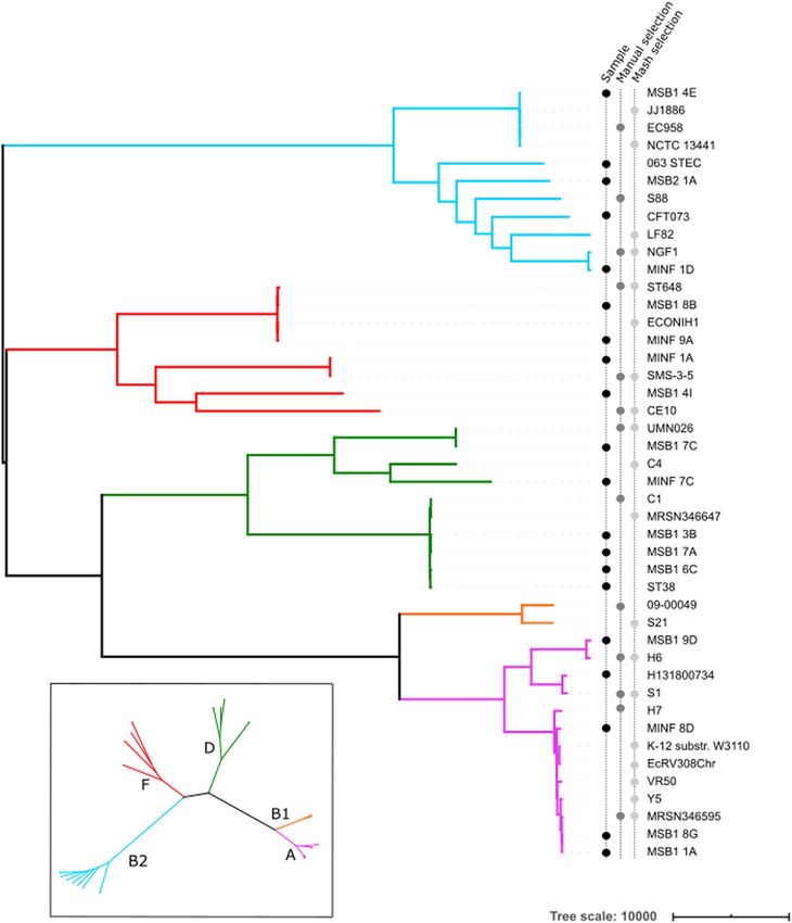
Colquhoun et al. Genome Biology   (2021) 22:267                                                                Page 3 of 30

                 graphs reduce the impact of soft reference bias on mapping [12, 14, 15], and on gener-
                 alizing alignment to graphs [16, 20]. These methods have almost universally been de-
                 signed for the human pan-genome, where hard reference bias is a comparatively minor
                 issue compared with bacteria (two human genomes are over 99% alignable, whereas
                 two bacteria of the same species might be 50% alignable). In particular, all current
                 graph methods (e.g., vg [12], Giraffe [21], GraphTyper [14, 15], paragraph [22], Bayes-
                 Typer [23]) require a reference genome to be provided in advance to output genetic
                 variants in the standard Variant Call Format (VCF) [24]—thus immediately inheriting a
                 hard bias when applied to bacteria (see Fig. 1B). Thus, there has not yet been any study
                 (to our knowledge) addressing SNP analysis across a diverse cohort, including more
                 variants that can fit on any single reference.
                   We have made a number of technical innovations. First, we use a recursive clustering
                 algorithm that converts a multiple sequence alignment (MSA) of a locus into a graph.
                 This avoids the complexity “blowups” that plague graph genome construction from
                 unphased VCF files [14,15]. Second, we introduce a graph representation of genetic
                 variation based on (w,k)-minimizers [25]. Third, using this representation, we avoid un-
                 necessary full alignment to the graph and instead use quasi-mapping to genotype on
                 the graph. Fourth, we use local assembly to discover variation missing from the refer-
                 ence graph. Fifth, we infer a canonical dataset-dependent reference genome designed to
                 maximize clarity of description of variants (the value of this will be made clear in the
                 main text).
                   We describe these below and evaluate our implementation, pandora, on a diverse set
                 of E. coli genomes with both Illumina and Nanopore data. We show that, compared
                 with reference-based approaches, pandora recovers a significant proportion of the
                 missing variation in rare loci, performs much more stably across a diverse dataset, suc-
                 cessfully infers a better reference genome for VCF output, and outperforms current
                 tools for Nanopore data.

                 Results
                 Pan-genome graph representation
                 We set out to define a generalized reference structure which allows detection of SNPs
                 and other variants across the whole pan-genome, without attempting to record long-
                 range structure or coordinates. We define a Pan-genome Reference Graph (PanRG) as an
                 unordered collection of sequence graphs, termed local graphs, each of which represents a
                 locus, such as a gene or intergenic region. Each local graph is constructed from a MSA of
                 known alleles of this locus, using a recursive cluster-and-collapse (RCC) algorithm (Add-
                 itional file 1: Supplementary Animation 1: recursive clustering construction). The output
                 is guaranteed to be a directed acyclic sequence graph allowing hierarchical nesting of gen-
                 etic variation while meeting a “balanced parentheses” criterion (see Fig. 2B and
                 “Methods”). Each path through the graph from source to sink represents a possible re-
                 combinant sequence for the locus. The disjoint nature of this pan-genome reference al-
                 lows loci such as genes to be compared regardless of their wider genomic context. We
                 implement this construction algorithm in the make_prg tool which outputs the graph as a
                 file (see Fig. 2A–C, “Methods”). We also implement a PanRG update algorithm in make_
                 prg which allows rapid augmentation of a pre-built PanRG with new alleles (see Fig. 2D,
Colquhoun et al. Genome Biology     (2021) 22:267                                                                               Page 4 of 30

                  Fig. 2 The pandora workflow. A Reference panel of genomes; color signifies locus (gene or intergenic
                  region) identifier, and blobs are SNPs. B The multiple sequence alignment (MSA) for each locus is converted
                  into a directed acyclic graph (termed local graph). C Local graphs constructed from the loci in the
                  reference panel. D Workflow: the collection of local graphs, termed the PanRG, is indexed. Reads from each
                  sample under study are independently quasi-mapped to the graph, and a determination is made as to
                  which loci are present in each sample. In this process, for each locus, a mosaic approximation of the
                  sequence for that sample is inferred, and variants are genotyped. E Regions of low coverage are detected,
                  and local de novo assembly is used to generate candidate novel alleles missing from the graph. Returning
                  to D, the dotted line shows all the candidate alleles from all samples are then gathered and added to the
                  PanRG. Then, reads are quasi-mapped one more time, to the augmented PanRG, generating new mosaic
                  approximations for all samples and storing coverages across the graphs; no de novo assembly is done this
                  time. A pan-genome matrix showing which input loci are present in each sample is created. Finally, all
                  samples are compared, and a VCF file is produced, with a per-locus reference that is inferred by pandora

                 “Methods”). Subsequent operations, based on this PanRG, are implemented in the soft-
                 ware package pandora. The overall workflow is shown in Fig. 2.
                   To index a PanRG, we generalize a type of sparse marker k-mer ((w,k)-minimizer, also
                 referred to as a minimizing k-mer), previously defined for strings, to directed acyclic
                 graphs (see “Methods”). Informally, each minimizer is the smallest k-mer in a window of
                 w consecutive k-mers. This has become a popular method for rapidly indexing and com-
                 paring genomes and long reads (e.g., MASH [26], minimap [27, 28]). It has the advantage
                 that the number of indexing k-mers scales with the length of the sequence so that differ-
                 ent length local graphs are each well represented in the index. In addition, it enables
                 shorter indexing k-mers to be used, which improves mapping with noisy reads.
                   Each local graph is sketched with minimizing k-mers, and these are then used to con-
                 struct a new graph (the k-mer graph) for each local graph from the PanRG. Each min-
                 imizing k-mer is a node, and edges are added between two nodes if they are adjacent
                 minimizers on a path through the original local graph. This k-mer graph is isomorphic
                 to the original if w ≤ k (and outside the first and last w + k − 1 bases); all subsequent
                 operations are performed on this graph, which, to avoid unnecessary new terminology,
                 we also call the local graph.
Colquhoun et al. Genome Biology   (2021) 22:267                                                                Page 5 of 30

                   A global index maps each minimizing k-mer to a list of all local graphs containing
                 that k-mer and the positions therein. Long or short reads are approximately mapped
                 (quasi-mapped) to the PanRG by determining the minimizing k-mers in each read. Any
                 of these read quasi-mappings found in a local graph are called hits, and any local graph
                 with sufficient clustered hits on a read is considered present in the sample.

                 Initial sequence approximation as a mosaic of references
                 For each locus identified as present in a sample, we initially approximate the sample’s
                 sequence as a path through the local graph. The result is a mosaic of sequences from
                 the reference panel. This path is chosen to have maximal support by reads, using a dy-
                 namic programming algorithm on the graph induced by its (w,k)-minimizers (details in
                 “Methods”). The result of this process serves as our initial approximation to the
                 genome under analysis.

                 Improved sequence approximation: modify mosaic by local assembly
                 At this point, we have quasi-mapped reads, and approximated the genome by finding
                 the closest mosaic in the graph; however, we expect the genome under study to contain
                 variants that are not present in the PanRG. Therefore, to allow discovery of novel SNPs
                 and small indels that are not in the graph, for each sample and locus, we identify re-
                 gions of the inferred mosaic sequence where there is a drop in read coverage (as shown
                 in Fig. 2E). Slices of overlapping reads are extracted, and a form of de novo assembly is
                 performed using a de Bruijn graph. Instead of trying to find a single correct path, the
                 de Bruijn graph is traversed (see “Methods” for details) to obtain all feasible candidate
                 novel alleles for the sample. These alleles are then added to the local graph. If compar-
                 ing multiple samples, the graphs are augmented with all new alleles from all samples at
                 the same time.

                 Optimal VCF reference construction for multi-genome comparison
                 In the compare step of pandora (see Fig. 2D), we enable continuity of downstream ana-
                 lysis by outputting genotype information in the conventional VCF [24]. In this format,
                 each row (record) describes possible alternative allele sequence(s) at a position in a
                 (single) reference genome and information about the type of sequence variant. A col-
                 umn for each sample details the allele seen in that sample, often along with details
                 about the support from the data for each allele.
                   To output graph variation, we first select a path through the graph to be the refer-
                 ence sequence and describe any variation within the graph with respect to this path as
                 shown in Fig. 3. We use the chromosome field to detail the local graph within the
                 PanRG in which a variant lies, and the position field to give the position in the chosen
                 reference path sequence for that graph. In addition, we output the reference path se-
                 quences used as a separate file.
                   For a collection of samples, we want small differences between samples to be re-
                 corded as short alleles in the VCF file rather than longer alleles with shared flanking se-
                 quence as shown in Fig. 3B. We therefore choose the reference path for each local
                 graph to be maximally close to the sample mosaic paths. To do this, we make a copy of
                 the k-mer graph and increment the coverage along each sample mosaic path, producing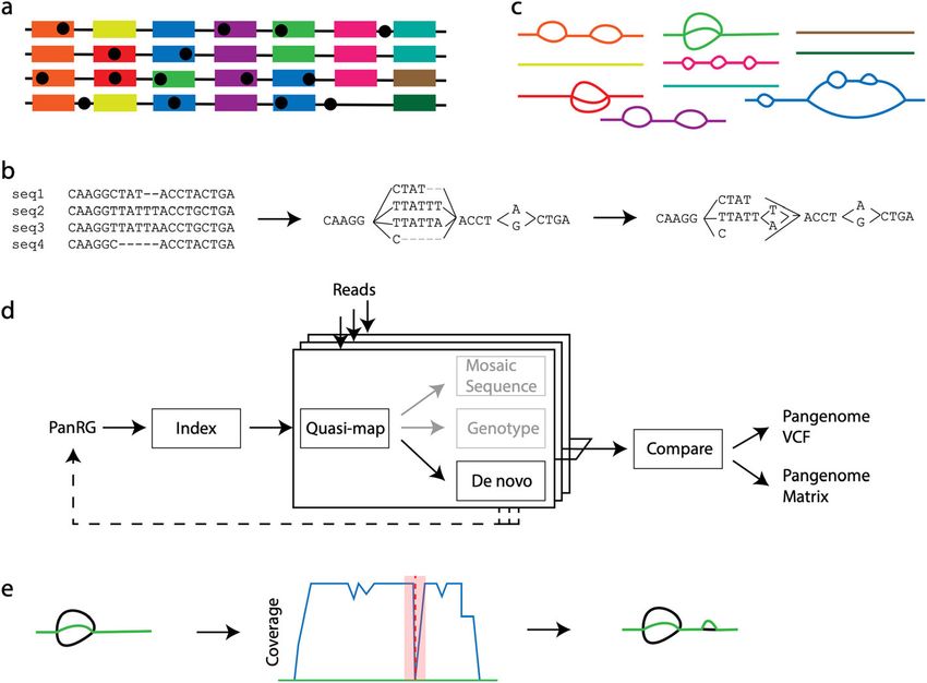
Colquhoun et al. Genome Biology      (2021) 22:267                                                                                Page 6 of 30

                  Fig. 3 The representation problem. A A local graph with sequence explicitly shown. B, C The same graph
                  with black reference path and alternate alleles in different colors, and the corresponding VCF records. In B,
                  the black reference path is distinct from both alleles. The blue/red SNP then requires flanking sequence in
                  order to allow it to have a coordinate. The SNP is thus represented as two ALT alleles, each 3 bases long,
                  and the user is forced to notice they only differ in one base. C The reference follows the blue path, thus
                  enabling a more succinct and natural representation of the SNP

                 a graph with higher weights on paths shared by more samples. We reuse the mosaic
                 path-finding algorithm (see “Methods”) with a modified probability function defined
                 such that the probability of a node is proportional to the number of samples covering
                 it. This produces a dataset-dependent VCF reference able to succinctly describe segre-
                 gating variation in the cohort of genomes under analysis.

                 Constructing a PanRG of E. coli
                 We chose to evaluate pandora on the recombining bacterial species, E. coli, whose pan-
                 genome has been heavily studied [7, 29–32]. MSAs for gene clusters curated with panX
                 [33] from 350 RefSeq assemblies were downloaded from http://pangenome.de on 3
                 May 2018. MSAs for intergenic region clusters based on 228 E. coli ST131 genome se-
                 quences were previously generated with Piggy [34] for their publication. While this
                 panel of intergenic sequences does not reflect the full diversity within E. coli, we in-
                 cluded them as an initial starting point. This resulted in an E. coli PanRG containing
                 local graphs for 23,051 genes and 14,374 intergenic regions. Pandora took 15 m in
                 CPU time (11 m in runtime with 16 threads) and 12.9 GB of RAM to index the PanRG.
                 As one would expect from the U-shaped gene frequency distribution, many of the
                 genes were rare in the 578 (=350 + 228) input genomes, and so 59%/44% of the genic/
                 intergenic graphs were linear, with just a single allele.

                 Constructing an evaluation set of diverse genomes
                 We first demonstrate that using a PanRG reduces hard bias when comparing a diverse
                 set of 20 E. coli samples by comparison with standard single-reference variant callers.
                 We selected samples from across the phylogeny (including phylogroups A, B2, D and F
                 [35]) where we were able to obtain both long- and short-read sequence data from the
                 same isolate.
                   We used Illumina-polished long-read assemblies as truth data, masking positions
                 where the Illumina data did not support the assembly (see “Methods”). As comparators,
                 we used SAMtools [36] (the “classical” variant caller based on pileups) and Freebayes
                 [37] (a haplotype-based caller which reduces soft reference bias, wrapped by snippy
                 [38]) for Illumina data, and medaka [39] and nanopolish [40] for Nanopore data. In all
                 cases, we ran the reference-based callers with 24 carefully selected reference genomes
                 (see “Methods” and Fig. 4). We defined a “truth set” of 618,305 segregating variants by
                 performing all pairwise whole genome alignments of the 20 truth assemblies, collecting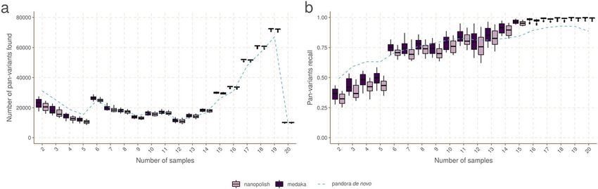
Colquhoun et al. Genome Biology     (2021) 22:267                                                                               Page 7 of 30

                  Fig. 4 Phylogeny of 20 diverse E. coli along with references used for benchmarking single-reference variant
                  callers. The 20 E. coli under study are labelled as samples in the left-hand of three vertical label-lines.
                  Phylogroups (clades) are labelled by color of branch, with the key in the inset. References were selected
                  from RefSeq as being the closest to one of the 20 samples as measured by Mash, or manually selected
                  from a tree (see “Methods”). Two assemblies from phylogroup B1 are in the set of references, despite there
                  being no sample in that phylogroup

                 SNP variants between the pairs, and deduplicating them by clustering into equivalence
                 classes. Each class, or pan-variant, represents the same variant found at different coor-
                 dinates in different genomes (see “Methods”). We evaluated error rate (proportion of
                 VCF records which are incorrect, see “Methods”), pan-variant recall (PVR, proportion
                 of segregating sites in the truth set discovered) and average allelic recall (AvgAR, aver-
                 age of the proportion of alleles of each pan-variant that are found). To clarify the defi-
                 nitions, consider a toy example. Suppose we have three genes, each with one SNP
                 between them. The first gene is rare, present in 2/20 genomes. The second gene is at
                 an intermediate frequency, in 10/20 genomes. The third is a strict core gene, present in
                 all genomes. The SNP in the first gene has alleles A,C at 50% frequency (1 A and 1 C).
                 The SNP in the second gene has alleles G,T at 50% frequency (5 G and 5 T). The SNP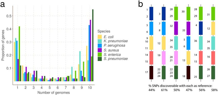
Colquhoun et al. Genome Biology (2021) 22:267 Page 8 of 30
in the third gene has alleles A,T with 15 A and 5 T. Suppose a variant caller found the
SNP in the first gene, detecting the two correct alleles. For the second gene’s SNP, it
detected only one G and one T, failing to detect either allele in the other 8 genomes.
For the third gene’s SNP, it detected all the 5 T’s, but no A. Here, the pan-variant recall
would be: (1 + 1 + 0) / 3 = 0.66—i.e., score a 1 if both alleles are found, irrespective of
how often- and the average allelic recall would be (2/2 + 2/10 + 5/20)/3 = 0.48. Thus
PVR and AvgAR are pan-genome equivalents of standard site discovery power and
genotyping accuracy.
Pandora detects rare variation inaccessible to single-reference methods
First, we evaluate the primary aim of pandora—the ability to access genetic variation
within the accessory genome. Figure 5 shows the PVR of SNPs in the truth set broken
down by the number of samples the SNP (either allele) is present in. Results are shown
for pandora, medaka, and nanopolish using Nanopore sequence data, and Additional
file 1: Supplementary Figure 1 shows an almost identical result for pandora, snippy,
and SAMtools using Illumina sequence data.
If we restrict our attention to rare variants (present only in 2–5 genomes), we find
pandora recovers at least 17.5/24.5/11.6/20.8 k more SNPs than SAMtools/snippy/me-
daka/nanopolish respectively. As a proportion of rare SNPs in the truth set, this is a lift
in PVR of 10.9/15.3/7.2/13.0% respectively. If, instead of pan-variant recall, we look at
the variation of AvgAR across the locus frequency spectrum (see Additional file 1: Sup-
plementary Figure 2), the gap between pandora and the other tools on rare loci is even
larger. These observations confirm and quantify the extent to which we are able to re-
cover accessory genetic variation that is inaccessible to single-reference-based methods.
Benchmarking recall, error rate, and dependence on reference
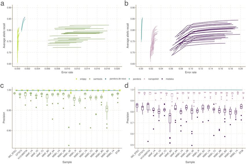
We show in Fig. 6A,B the Illumina and Nanopore AvgAR/error rate plots for pandora
and four single-reference tools with no filters applied. For all of these, we modify only
the minimum genotype confidence to move up and down the curves (see “Methods”).
We highlight three observations. Firstly, pandora achieves essentially the same recall
and error rate for the Illumina and Nanopore data (85% AvgAR and 0.2–0.3% error rate
Fig. 5 Pan-variant recall across the locus frequency spectrum. Every SNP occurs in a locus, which is present
in some subset of the full set of 20 genomes. SNPs in the golden truth set are broken down by the
number of samples the locus is present in. In panel A, we show the absolute count of pan-variants found
and in panel B we show the proportion of pan-variants found (PVR) for pandora (dotted line), nanopolish,
and medaka with Nanopore data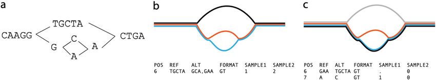
Colquhoun et al. Genome Biology      (2021) 22:267                                                                                    Page 9 of 30

                  Fig. 6 Benchmarks of recall/error rate and dependence of precision on reference genome, for pandora and
                  other tools on 20-way dataset. A The average allelic recall and error rate curve for pandora, SAMtools, and
                  snippy on 100× of Illumina data. Snippy/SAMtools both run 24 times with the different reference genomes
                  shown in Fig. 4, resulting in multiple lines for each tool (one for each reference). B The average allelic recall
                  and error rate curve for pandora, medaka, and nanopolish on 100× of Nanopore data; multiple lines for
                  medaka/nanopolish, one for each reference genome. Note panels A and B have the same y-axis scale and
                  limits, but different x axes. C The precision of pandora, SAMtools, and snippy on 100× of Illumina data. The
                  boxplots show the distribution of SAMtools’ and snippy’s precision depending on which of the 24 references
                  was used, and the blue line connects pandora’s results. D The precision of pandora (line plot), medaka, and
                  nanopolish (both boxplots) on 100× of Nanopore data. Note different y-axis scale/limits in panels C and D

                 at the top-right of the curve, completely unfiltered). Second, choice of reference has a
                 significant effect on both AvgAR and error rate for the single-reference callers; the ref-
                 erence which enables the highest recall does not lead to the best error rate. Third, pan-
                 dora achieves better AvgAR (85%) than all other tools (all between 73 and 84%, see
                 Additional file 1: Supplementary Table 1), and a better error rate (0.2–0.3%) than SAM-
                 tools (1.0%), nanopolish (2.4%), and medaka (14.8%). However, snippy achieves a signifi-
                 cantly better error rate than all other tools (0.01%). We confirmed that adding further
                 filters slightly improved error rates, but did not change the overall picture (Additional
                 file 1: Supplementary Figure 3, “Methods”, Additional file 1: Supplementary Table 1).
                 The results are also in broad agreement if the PVR is plotted instead of AvgAR (Add-
                 itional file 1: Supplementary Figure 4). However, these AvgAR and PVR figures are
                 hard to interpret because pandora and the reference-based tools have recall that varies
                 differently across the locus frequency spectrum, as described above. We explore this
                 further below.
                    We ascribe the similarity between the Nanopore and Illumina performance of pan-
                 dora to three reasons. First, the PanRG is a strong prior—our first approximation does
                 not contain any Nanopore sequence, but simply uses quasi-mapped reads to find the
                 nearest mosaic in the graph. Second, mapping long Nanopore reads which completely
                 cover entire genes is easier than mapping Illumina data and allows us to filter out errone-
                 ous k-mers within reads after deciding when a gene is present. Third, this performance is
Colquhoun et al. Genome Biology (2021) 22:267 Page 10 of 30
only achieved when we use methylation-aware basecalling of Nanopore reads, presumably
removing most systematic bias (see Additional file 1: Supplementary Figure 5).
In Fig. 6C,D, we show for Illumina and Nanopore data, the impact of reference choice on
the precision of calls on each of the 20 samples. While precision is consistent across all sam-
ples for pandora, we see a dramatic effect of reference choice on precision of SAMtools, me-
daka, and nanopolish. The effect is also detectable for snippy, but to a much lesser extent.
Finally, we measured the performance of locus presence detection, restricting to
genes/intergenic regions in the PanRG, so that in principle perfect recall would be pos-
sible (see “Methods”). In Additional file 1: Supplementary Figure 6, we show the distri-
bution of locus presence calls by pandora, split by length of locus for Illumina and
Nanopore data. Overall, 93.7%/94.3% of loci were correctly classified as present or ab-
sent for Illumina/Nanopore respectively. Misclassifications were concentrated on small
loci (below 500 bp). While 59.5%/57.4% of all loci in the PanRG are small, 75.5%/75.7%
of false positive calls and 99.1%/98.5% of false negative calls are small loci (see Add-
itional file 1: Supplementary Figure 6).
Pandora has consistent results across E. coli phylogroups
We measure the impact of reference bias (and population structure) by quantifying
how recall varies in phylogroups A, B2, D, and F depending on whether the reference
genome comes from the same phylogroup.
We plot the results for snippy with 5 exemplar references in Fig. 7A (results for all
tools and for all references are in Additional file 1: Supplementary Figures 7-10), show-
ing that single references give 5–10% higher recall for samples in their own phylogroup
than other phylogroups. By comparison, pandora’s recall is much more consistent, stay-
ing stable at ~ 90% for all samples regardless of phylogroup. References in phylogroups
A and B2 achieve higher recall in their own phylogroup, but consistently worse than
pandora for samples in the other phylogroups (in which the reference does not lie).
Fig. 7 Single-reference callers achieve higher recall for samples in the same phylogroup as the reference
genome, but not for rare loci. A Pandora recall (black line) and snippy recall (colored bars) of pan-variants in
each of the 20 samples; each histogram corresponds to the use of one of 5 exemplar references, one from
each phylogroup. The background color denotes the reference’s phylogroup (see Fig. 4 inset); note that
phylogroup B1 (yellow background) is an outgroup, containing no samples in this dataset. B Same as A but
restricted to SNPs present in precisely two samples (i.e., where 18 samples have neither allele because the
entire locus is missing). Note the differing y-axis limits in the two panelsColquhoun et al. Genome Biology (2021) 22:267 Page 11 of 30
References in the external phylogroup B1, for which we had no samples in our dataset,
achieve higher recall for samples in the nearby phylogroup A (see inset, Fig. 4), but
lower than pandora for all others. We also see that choosing a reference genome from
phylogroup F, which sits intermediate to the other phylogroups, provides the most uni-
form recall across other groups—2–5% higher than pandora.
These results will, however, be dominated by the shared, core genome. If we replot Fig. 7A,
restricting to variants in loci present in precisely 2 genomes (abbreviated to 2-variants; Fig.
7B), we find that pandora achieves 49–86% recall for each sample (complete data in Add-
itional file 1: Supplementary Figure 11). By contrast, for any choice of reference genome, the
results for single-reference callers vary dramatically per sample, ranging from 4 to 83% for
snippy for example. Most sample-reference pairs (388/480) have recall under 49% (the lower
bound for pandora recall), and there is no pattern of improved recall for samples in the same
phylogroup as the reference. Following up that last observation, if we look at which pairs of
genomes share 2-variants (Fig. 8), we find there is no enrichment within phylogroups at all.
This simply confirms in our data that presence of rare loci is not correlated with the overall
phylogeny. For completeness, Additional file 1: Supplementary Animation 2 shows the pan-
dora and snippy recall for all 24 references, split by variant frequency.
Pandora VCF reference is closer to samples than any single reference
The relationship between phylogenetic distance and gene repertoire similarity is not
linear. In fact, 2 genomes in different phylogroups may have more similar accessory
genes than 2 in the same phylogroup—as illustrated in the previous section (also see
Fig. 3 in Rocha [3]). As a result, it is unclear a priori how to choose a good reference
Fig. 8 Sharing of variants present in precisely 2 genomes, showing which pairs of genomes they lie in and
which phylogroups; darker colors signify higher counts (log scale). Axes are labelled with genome
identifiers, colored by their phylogroup (see Fig. 4 inset)Colquhoun et al. Genome Biology (2021) 22:267 Page 12 of 30
genome for comparison of accessory loci between samples. Pandora specifically aims to
construct an appropriate reference for maximum clarity in VCF representation. We
evaluate how well pandora is able to find a VCF reference close to the samples under
study as follows. We first identified the location of all loci in all the 20 sample assem-
blies and the 24 references (see “Methods”).
We then measured the edit distance between each locus in each of the references and
the corresponding version in the 20 samples. We found that the pandora’s VCF refer-
ence lies within 1% edit distance (scaled by locus length) of the sample far more than
any of the references for loci present in ≤ 9 samples (Fig. 9; note the log scale). Add-
itional file 1: Supplementary Figure 12 shows a similar result for 0% edit distance (exact
match). In both cases, the improvement is much reduced in the core genome; essen-
tially, in the core, a phylogenetically close reference provides a good approximation,
but it is hard to choose a single reference that provides a close approximation to all
rare loci. By contrast, pandora is able to leverage its reference panel, and the dataset
under study, to find a good approximation.
Computational performance
We report here the CPU time and maximum RAM consumed by the evaluated tools.
All of the single-reference tools analyzed isolates independently, whereas pandora has a
subsequent joint analysis step to compare them all; we therefore compare the end-to-
end performance of pandora analyzing all 20 samples against the mean performance of
each single-reference tool (summing all 20 samples, and then averaging over the differ-
ent reference genomes). In short, pandora took 9.2 CPU hours to analyze the 20
Fig. 9 How often do references closely approximate a sample? Pandora aims to infer a reference for use in
its VCF, which is as close as possible to all samples. We evaluate the success of this here. The x-axis shows
the number of genomes in which a locus occurs. The y-axis shows the (log-scaled) count of loci in the 20
samples that are within 1% edit distance (scaled by locus length) of each reference—box plots for the
reference genomes, and line plot for the VCF reference inferred by pandoraColquhoun et al. Genome Biology (2021) 22:267 Page 13 of 30
isolates with Illumina data while snippy and SAMtools both took 0.4 CPU hours. With
Nanopore data, pandora took 16.4 CPU hours, which is slower than medaka (0.7 CPU
hours), but faster than nanopolish (84 CPU hours). In terms of memory usage, for the
Illumina data, pandora used a maximum of 13.4 GB of RAM, compared with snippy
(3.2 GB), and SAMtools (1.0 GB), whereas for the Nanopore data, pandora used a max-
imum of 15.7 GB of RAM, compared with medaka (5.9 GB) and nanopolish (10.4 GB).
Discussion
Bacteria are the most diverse and abundant cellular life form [41]. Some species are ex-
quisitely tuned to a particular niche (e.g., obligate pathogens of a single host) while
others are able to live in a wide range of environments (e.g., E. coli can live on plants,
in the earth, or commensally in the gut of various hosts). Broadly speaking, a wider
range of environments correlates with a larger pan-genome, and some parts of the gene
repertoire are associated with specific niches [42]. Our perception of a pan-genome
therefore depends on our sampling of the unknown underlying population structure,
and similarly the effectiveness of a PanRG will depend on the choice of reference panel
from which it is built.
Many examples from different species have shown that bacteria are able to leverage
this genomic flexibility, adapting to circumstance sometimes by using or losing novel
genes acquired horizontally, and at other times by mutation. There are many situations
where precise nucleotide-level variants matter in interpreting pan-genomes. Some ex-
amples include compensatory mutations in the chromosome reducing the fitness bur-
den of new plasmids [43–45]; lineage-specific accessory genes with SNP mutations
which distinguish carriage from infection [46]; SNPs within accessory drug resistance
genes leading to significant differences in antibiograms [47]; and changes in CRISPR
spacer arrays showing immediate response to infection [48, 49]. However, up until
now, there has been no automated way of studying non-core gene SNPs at all; still less
a way of integrating them with gene presence/absence information. Pandora solves
these problems, allowing detection and genotyping of core and accessory variants. It
also addresses the problem of what reference to use as a coordinate system, inferring a
mosaic “VCF reference” which is as close as possible to all samples under study. We
find this gives more consistent SNP calling than any single reference in our diverse
dataset. We focussed primarily on Nanopore data when designing pandora and show it
is possible to achieve higher quality SNP calling with this data than with current Nano-
pore tools. The impact of this approach does depend on the dataset under study. We
find that, if analyzing closely related samples, then single-reference methods provide
improved recall compared with pandora. However, if analyzing more diverse datasets,
hard reference bias is a bigger issue for single-reference tools, and pandora offers im-
proved recall.
Prior graph genome work, focussing on soft reference bias (in humans), has evaluated
different approaches for selecting alleles for addition to a population graph, based on
frequency, avoiding creating new repeats, and avoiding exponential blow-up of haplo-
types in clusters of variants [50]. This approach makes sense when you have unphased
diploid VCF files and are considering all recombinants of clustered SNPs as possible.
However, this is effectively saying we consider the recombination rate to be high
enough that all recombinants are possible. Our approach, building from local MSAsColquhoun et al. Genome Biology (2021) 22:267 Page 14 of 30
and only collapsing haplotypes when they agree for a fixed number of bases, preserves
more haplotype structure and avoids combinatorial explosion. Another alternative ap-
proach was recently taken by Norri et al. [51], inferring a set of pseudo founder ge-
nomes from which to build the graph.
With pandora, we break the genome into atomic units which may reorder freely be-
tween samples, but within which the degree of variation is more constrained. This ap-
proach is directly motivated by our knowledge of the mechanisms underlying genomic
flexibility in bacteria. The breadth of diversity we see in these bacteria arises primarily
as a result of horizontally acquired DNA which is incorporated into the genome by dif-
ferent forms of recombination. Homologous recombination between closely related se-
quences may result in allele conversion and in some species contributes as many
nucleotide changes as point mutation [52]. As a result, locally we expect sequences to
look like mosaics of each other, possibly with additional novel mutations. Genes are ac-
quired (and lost) as a result of homologous or site-specific recombination and at hot-
spots [53, 54]. The dynamics of this are organized [30], and result in global genome
mosaicism. The choice of atomic unit used to build each local graph should again be
motivated by this underlying biology. A locus should be large enough for its presence
and sequence to be useful independently of other graphs, but small enough as to be
typically inherited as an entire unit. Biologically speaking, genes fulfil this requirement
and there already exist a plethora of tools designed to extract and align genes (and
intergenic regions) in a set of bacterial genomes (prokka [55], panaroo [56], roary [57],
panX [33], piggy [34]). Operons or groups of genes which co-occur contiguously might
also make a good choice, although isolating a set of reference sequences for these re-
gions would be more of a challenge.
Another issue is how to select the reference panel of genomes in order to minimize
hard reference bias. One cannot escape the U-shaped frequency distribution; whatever
reference panel is chosen, future genomes under study will contain rare genes not
present in the PanRG. Given the known strong population structure in bacteria, and
the association of accessory repertoires with lifestyle and environment, we would advo-
cate sampling by phylogeny, geography, host species (if appropriate), lifestyle (e.g.,
pathogenic versus commensal), and/or environment. In this study, we built our PanRG
from a biased dataset (RefSeq) which does not attempt to achieve balance across phyl-
ogeny or ecology, limiting our pan-variant recall to 49% for rare variants (see Fig. 5B,
Additional file 1: Supplementary Figure 1C). A larger, carefully curated input panel,
such as that from Horesh et al. [58], would provide a better foundation and potentially
improve results.
A natural question is then to ask if the PanRG should continually grow, absorbing all
variants ever encountered. From our perspective, the answer is no—a PanRG with vari-
ants at all non-lethal positions would be potentially intractable. The goal is not to have
every possible allele in the PanRG—no more than a dictionary is required to contain
absolutely every word that has ever been said in a language. As with dictionaries, there
is a trade-off between completeness and utility, and in the case of bacteria, the language
is far richer than English. The perfect PanRG contains the vast majority of the genes
and intergenic regions you are likely to meet, and just enough breadth of allelic diver-
sity to ensure reads map without too many mismatches. Missing alleles should be dis-
coverable by local assembly and added to the graph, allowing multi-sample comparisonColquhoun et al. Genome Biology (2021) 22:267 Page 15 of 30
of the cohort under study. This allows one to keep the main PanRG lightweight enough
for rapid and easy use.
For bacterial genomes, genotype calls are often used to perform phylogenetic ana-
lyses. By detecting accessory variation, three things become possible. First, pragmatic-
ally, one can choose clusters of similar genomes based on the cohort-wide core
genome, and then by restricting the pandora VCF to genes present in each cluster, re-
analyze based on the cluster-specific core genome. Normally this would require choos-
ing a cluster-specific reference, remapping reads and re-running a variant caller, but
with pandora all of the necessary data is provided in one step. Secondly, the accessory
SNPs provide an extra level of resolution when comparing samples which are very close
on a core genome tree, which may be useful. Finally, one cannot represent all pan-
genome variation in a phylogeny as the evolutionary history is fundamentally not com-
patible with a simple vertical-inheritance model. However, the pandora output would
make ideal material on which to build and test population genetic models.
We finish with potential applications of pandora. First, the PanRG should provide a
more interpretable substrate for pan-genome-wide genome-wide association studies, as
current methods are forced to either ignore the accessory genome or reduce it to k-mers
or unitigs [59–61] abstracted from their wider context. Second, it would allow investiga-
tion of selection and adaptation of accessory SNPs. Third, if performing prospective sur-
veillance of microbial isolates taken in a hospital, the PanRG provides a consistent and
unchanging reference, which will cope with the diversity of strains seen without requiring
the user to keep switching reference genome. Finally, if studying a fixed dataset very care-
fully, then one may not want to use a population PanRG, as it necessarily will miss some
rare accessory genes in the dataset. In these circumstances, one could construct a refer-
ence graph purely of the genes/intergenic regions present in this dataset.
There are a number of limitations to this study. Firstly, although pandora achieves a
gain of recall in rare variation compared with single-reference tools (at least 12–25 k
more SNPs in loci present in 2–5 genomes out of 20 depending on choice of tool and
reference—a lift of at least 7–15% in recall), this is offset by 11% loss of recall at core
SNPs. However, the gain in recall of rare variants will increase both with dataset size
(due to the U-shaped gene frequency curve) and with a PanRG constructed from either
a better-sampled input reference panel, or the dataset itself. By contrast, there is no a
priori reason why pandora should miss core SNPs, and this issue will need to be ad-
dressed in future work. Finally, by working in terms of atomic loci instead of a mono-
lithic genome-wide graph, pandora opens up graph-based approaches to structurally
diverse species (and eases parallelisation) but at the cost of losing genome-wide order-
ing. At present, ordering can be resolved by (manually) mapping pandora-discovered
genes onto whole genome assemblies. However the design of pandora also allows for
gene-ordering inference: when Nanopore reads cover multiple genes, the linkage be-
tween them is stored in a secondary de Bruijn graph where the alphabet consists of
gene identifiers. This results in a huge alphabet, but the k-mers are almost always
unique, dramatically simplifying “assembly” compared with normal DNA de Bruijn
graphs. This work is still in progress and the subject of a future study. In the meantime,
pandora provides new ways to access previously hidden variation.Colquhoun et al. Genome Biology (2021) 22:267 Page 16 of 30
Conclusions
The algorithms implemented in pandora provide a solution to the problem of analyzing core
and accessory genetic variation across a set of bacterial genomes. This study demonstrates as
good SNP genotype error rates with Nanopore as with Illumina data and improved recall of
accessory variants. It also shows the benefit of an inferred VCF reference genome over simply
picking from RefSeq. The main limitations were the use of a biased reference panel (RefSeq)
for building the PanRG, and a slightly lower recall for core SNPs than single-reference tools—
both of which are addressable, not fundamental limitations. This work opens the door to im-
proved analyses of many existing and future bacterial genomic datasets.
Methods
Local graph construction
We construct each local graph in the PanRG from an MSA using an iterative partitioning
process. The resulting sequence graph contains nested bubbles representing alternative alleles.
Let A be an MSA of length n. For each row of the MSA a = {a0, …, an−1} ∈ A let ai, j =
{ai, …, aj−1} be the subsequence of a in interval [i, j). Let s(a) be the DNA sequence ob-
tained by removing all non-AGCT symbols. We can partition alignment A either verti-
cally by partitioning the interval [0, n) or horizontally by partitioning the set of rows of
A. In both cases, the partition induces a number of sub-alignments.
For vertical partitions, we define sliceA(i, j) = {ai,j : a ∈ A}. We say that interval [i, j) is a
match interval if j − i ≥ m, where m = 7 is the default minimum match length, and there
is a single non-trivial sequence in the slice, i.e.,
jfsðaÞ : a ∈ sliceA ði; jÞ and sðaÞ≠””gj ¼ 1:
Otherwise, we call it a non-match interval.
For horizontal partitions, we use a reference-based approach combined with K-means
clustering [62] to divide sequences into increasing numbers of clusters K = 2, 3, … until
each cluster meets a “one-reference-like” criterion or until K = 10. More formally, let U
be the set of all m-mers (substrings of length m, the minimum match length) in {s(a) :
a ∈ A}. For a ∈ A, we transform sequence s(a) into a count vector xa ¼ fxa 1 ; …; xa jUj g
where xai is the count of unique m-mer i ∈ U. The K-means algorithm partitions {s(a) :
¼ fC 1 ; …; C K g by minimizing the inertia, defined as
a ∈ A} into K clusters C
XK X 2
arg minC j¼1
xa −μ j
xa ∈C j
P
where μ j ¼ jC1 j j xa ∈C j xa is the mean of cluster j.
Given a (sub-)alignment A, we define the reference of A, ref(A), to be the concaten-
ation of the most frequent nucleotide at each position of A. We say that a K-partition
is one-reference-like if for the corresponding sub-alignments A1, …, AK the hamming
distance between each sequence and its sub-alignment reference
jsðaÞ−re f ðAi Þj < dlenðAÞ ∀a ∈ Ai
where | | denotes the Hamming distance, and d denotes a maximum hamming distance
threshold, set at 0.2 by default. In this case, we accept the partition; otherwise, we look
for a K + 1-partition.Colquhoun et al. Genome Biology (2021) 22:267 Page 17 of 30
The recursive algorithm first partitions an MSA vertically into match and non-match
intervals. Match intervals are collapsed down to the single sequence they represent. In-
dependently for each non-match interval, the alignment slice is partitioned horizontally
into clusters. The same process is then applied to each induced sub-alignment until a
maximum number of recursion levels, r = 5, has been reached. For any remaining align-
ments, a node is added to the local graph for each unique sequence. See Additional file
1: Supplementary Animation 1 to see an example of this algorithm. We name this algo-
rithm Recursive Cluster and Collapse (RCC). When building the local graph from a
MSA, we record and serialize the recursion tree of the RCC algorithm, as well as mem-
oizing all the data in each recursion node. We shall call this algorithm memoized RCC
(MRCC). Once the MRCC recursion tree is generated, we can obtain the local graph
through a pre-order traversal of the tree (which is equivalent to the call order of the re-
cursive functions in an execution of the RCC algorithm). To update the local graph
with new alleles using the MRCC algorithm, we can deserialize the recursion tree from
disk, infer in which leaves of the recursion tree the new alleles should be added, add
the new alleles in bulk, and then update each modified leaf. This leaf update operation
consists of updating just the subaligment of the leaf (which is generally a small fraction
of the whole MSA) with the new alleles using MAFFT [63] and recomputing the recur-
sion at the leaf node. All of this is implemented in the make_prg repository (see “Code
availability”).
(w,k)-minimizers of graphs
We define (w,k)-minimizers of strings as in Li [27]. Let φ : Σk →R be a k-mer hash
function and let π : Σ∗ × {0, 1} → Σ∗ be defined such that π(s, 0) = s and πðs; 1Þ ¼ s, where
s is the reverse complement of s. Consider any integers k ≥ w > 0. For window start pos-
ition 0 ≤ j ≤ |s| − w − k + 1, let
T j ¼ π sp;pþk ; r : j≤ p < j þ w; r∈f0; 1g
be the set of forward and reverse-complement k-mers of s in this window. We define a
(w,k)-minimizer to be any triple (h, p, r) such that
h ¼ φ π sp;pþk ; r ¼ min φðt Þ : t ∈ T j :
The set W(s) of (w,k)-minimizers for s, is the union of minimizers over such
windows:
W ðsÞ ¼ ⋃
0 ≤ j ≤ jsj−w−kþ1
fðh; p; rÞ : h ¼ minfφðtÞ : t ∈ T j gg:
We extend this definition intuitively to an acyclic sequence graph G = (V,E). Define
|v| to be the length of the sequence associated with node v ∈ V and let i = (v, a, b), 0 ≤
a ≤ b ≤ |v| represent the sequence interval [a, b) on v. We define a path in G by
¼ ði1 ; …; im Þ : v j ; v jþ1 ∈E and b j ≡ jv j j for 1 ≤ j < m :
p
This matches the intuitive definition for a path in a sequence graph except that we
allow the path to overlap only part of the sequence associated with the first and last
in the graph.
to refer to the sequence along the path p
nodes. We will use spColquhoun et al. Genome Biology (2021) 22:267 Page 18 of 30
Let q be a path of length w + k − 1 in G. The string sq contains w consecutive k-mers
for which we can find the (w,k)-minimizer(s) as before. We therefore define the (w,k)-
minimizer(s) of the graph G to be the union of minimizers over all paths of length w +
k − 1 in G:
W ðGÞ ¼ ⋃
q∈G :∣
q ∣¼wþk−1
; rÞ : h ¼ minfφðtÞ : t∈T q gg:
fðh; p
Local graph indexing with (w,k)-minimizers
To find minimizers for a graph, we use a streaming algorithm as described in Add-
itional file 1: Supplementary Algorithm 1. For each minimizer found, it simply finds the
next minimizer(s) until the end of the graph has been reached.
Let walk(v, i, w, k) be a function which returns all vectors of w consecutive k-mers in
G starting at position i on node v. Suppose we have a vector of k-mers x. Let shift(x) be
the function which returns all possible vectors of k-mers which extend x by one k-mer.
It does this by considering possible ways to walk one letter in G from the end of the
final k-mer of x. For a vector of k-mers of length w, the function minimize(x) returns
the minimizing k-mers of x.
We define K to be a k-mer graph with nodes corresponding to minimizers ðh; p ; rÞ.
We add edge (u,v) to K if there exists a path in G for which u and v are both mini-
mizers and v is the first minimizer after u along the path. Let K ← add(s, t) denote the
addition of nodes s and t to K and the directed edge (s,t). Let K ← add(s, T) denote the
addition of nodes s and t ∈ T to K as well as directed edges (s,t) for t ∈ T, and define
K ← add(S, t) similarly.
The resulting PanRG index stores a map from each minimizing k-mer hash value to
the positions in all local graphs where that (w,k)-minimizer occurred. In addition, we
store the induced k-mer graph for each local graph.
Quasi-mapping reads
We infer the presence of PanRG loci in reads by quasi-mapping. For each read, a sketch
of (w,k)-minimizers is made, and these are queried in the index. For every (w,k)-
minimizer shared between the read and a local graph in the PanRG index, we define a
hit to be the coordinates of the minimizer in the read and local graph and whether it
was found in the same or reverse orientation. We define clusters of hits from the same
read, local graph, and orientation if consecutive read coordinates are within a certain
distance. If this cluster is of sufficient size, the locus is deemed to be present and we
keep the hits for further analysis. Otherwise, they are discarded as noise. The default
for this “sufficient size” is at least 10 hits and at least 1/5th the length of the shortest
path through the k-mer graph (Nanopore) or the number of k-mers in a read sketch
(Illumina). Note that there is no requirement for all these hits to lie on a single path
through the local graph. A further filtering step is therefore applied after the sequence
at a locus is inferred to remove false positive loci, as indicated by low mean or median
coverage along the inferred sequence by comparison with the global average coverage.
This quasi-mapping procedure is described in pseudocode in Additional file 1: Supple-
mentary Algorithm 2.Colquhoun et al. Genome Biology (2021) 22:267 Page 19 of 30
Initial sequence approximation as a mosaic of references
For each locus identified as present in the set of reads, quasi-mapping provides (fil-
tered) coverage information for nodes of the directed acyclic k-mer graph. We use
these to approximate the sequence as a mosaic of references as follows. We model k-
mer coverage with a negative binomial distribution and use the simplifying assumption
that k-mers are read independently. Let Θ be the set of possible paths through the k-
mer graph, which could correspond to the true genomic sequence from which reads
were generated. Let r + s be the number of times the underlying DNA was read by the
machine, generating a k-mer coverage of s, and r instances where the k-mer was se-
quenced with errors. Let 1 − p be the probability that a given k-mer was sequenced cor-
rectly. For any path θ ∈ Θ, let {X1, …, XM} be independent and identically distributed
random variables with probability distribution f ðxi ; r; pÞ ¼ ΓðrþsÞ s
ΓðrÞs! p ð1−pÞ , representing
r
ð1−pÞr ð1−pÞr
the k-mer coverages along this path. Since the mean and variance are p and p2 ,
we solve for r and p using the observed k-mer coverage mean and variance across all k-
mers in all graphs for the sample. Let D be the k-mer coverage data seen in the read
P
dataset. We maximize the score θ^ ¼ farg max lðθjDÞg where lðθjDÞ ¼ 1 M
θ∈Θ M i¼1
log f ðsi ; r; pÞ , where si is the observed coverage of the i-th k-mer in θ. This score is an
approximation to a log likelihood, but averages over (up to) a fixed number of k-mers in
order to retain sensitivity over longer paths in our C++ implementation. By construction,
the k-mer graph is directed and acyclic so this maximization problem can be solved
with a dynamic programming algorithm (for pseudocode, see Additional file 1: Supple-
mentary Algorithm 3).
For choices of w ≤ k there is a unique sequence along the discovered path through
the k-mer graph (except in rare cases within the first or last w − 1 bases). We use this
closest mosaic of reference sequences as an initial approximation of the sample
sequence.
De novo variant discovery
The first step in our implementation of local de novo variant discovery in genome
graphs is finding the candidate regions of the graph that show evidence of dissimilarity
from the sample’s reads.
Finding candidate regions
The input required for finding candidate regions is a local graph, n, within the PanRG,
the maximum likelihood path of both sequence and k-mers in n, lmpn and kmpn re-
spectively, and a padding size w for the number of positions surrounding the candidate
region to retrieve.
We define a candidate region, r, as an interval within n where coverage on lmpn is
less than a given threshold, c, for more than l and less than m consecutive positions. m
acts to restrict the size of variants we are able to detect. If set too large, the following
steps become much slower due to the combinatorial expansion of possible paths. For a
given read, s, that has a mapping to r we define sr to be the subsequence of s that maps
to r, including an extra w positions either side of the mapping. We define the pileup Pr
as the set of all sr ∈ r.You can also read