Overcoming the effect of pupil distortion in multiconjugate adaptive optics
←
→
Page content transcription
If your browser does not render page correctly, please read the page content below
Overcoming the effect of pupil distortion in multiconjugate
                                                                      adaptive optics
                                                 Marcos A. van Dama , Yolanda Martı́n Hernandob , Miguel Núñez Cagigalb , and Luzma M.
                                                                                       Montoyab
                                                              a
                                                                Flat Wavefronts, 21 Lascelles Street, Christchurch 8022, New Zealand
                                                      b
                                                          Instituto de Astrofı́sica de Canarias, C/ Vı́a Láctea s/n 38205, La Laguna, Spain
arXiv:2201.05913v1 [astro-ph.SR] 15 Jan 2022

                                                                                               ABSTRACT
                                               Multiconjugate adaptive optics (MCAO) systems have the potential to deliver diffraction-limited images over
                                               much larger fields of view than traditional single conjugate adaptive optics systems. In MCAO, the high altitude
                                               deformable mirrors (DMs) cause a distortion of the pupil plane and lead to a dynamic misregistration between the
                                               DM actuators and the wavefront sensors (WFSs). The problem is much more acute for solar astronomy than for
                                               night-time observations due to the higher spatial sampling of the WFSs and DMs, and the fact that the science
                                               observations are often made through stronger turbulence and at lower elevations. The dynamic misregistration
                                               limits the quality of the correction provided by solar MCAO systems.
                                                  In this paper, we present PropAO, the first AO simulation tool (to our knowledge) to model the effect of
                                               pupil distortion. It takes advantage of the Python implementation of the optical propagation library PROPER.
                                               PropAO uses Fresnel propagation to propagate the amplitude and phase of an incoming wave through the
                                               atmosphere and the MCAO system. The resulting wavefront is analyzed by the WFSs and also used to evaluate
                                               the corrected image quality. We are able to reproduce the problem of pupil distortion and test novel non-linear
                                               reconstruction strategies that take the distortion into account. PropAO is shown to be an essential tool to study
                                               the behavior of the wavefront reconstruction and control for the European Solar Telescope.
                                               Keywords: multiconjugate adaptive optics, solar, wavefront reconstruction, pupil distortion

                                                                                          1. INTRODUCTION
                                               Multiconjugate adaptive optics (MCAO) uses two or more deformable mirrors (DMs) at different conjugate
                                               altitudes in order to correct the three-dimensional structure of turbulence and hence increase the corrected
                                               field-of-view relative to conventional single conjugate adaptive optics (SCAO).
                                                   MCAO has enjoyed some success in night time astronomy, with the MAD demonstrator at the VLT1 and
                                               GeMS2, 3 on Gemini South paving the way. GeMS has been routinely producing corrected science images over an
                                               8500 ×8500 field since 2013. Solar MCAO has an even longer history,4, 5 although early experiments were hampered
                                               by problems with loop stability. The 3 DM MCAO system Clear at the Goode Solar Telescope has provided
                                               high-order AO correction over a 3000 times3000 at visible wavelengths since 2016.6
                                                  The combination of one or more DMs at a very high altitude and the small subaperture sizes in solar MCAO
                                               can lead to an unstable loop in the presence of moderate to strong seeing. Table 1 records the salient differences
                                               between night-time and solar MCAO that affect the loop stability.

                                                                            Parameter                         Night-time     Solar
                                                                          Highest DM conjugate altitude         9 km 25 km
                                                                          Subaperture size                    0.50 m 0.10 m
                                                     Table 1: Comparison of relevant parameters for the MCAO systems on Gemini South and Gregor.7
                                                  Further author information: send correspondence to Marcos van Dam: marcos@flatwavefronts.com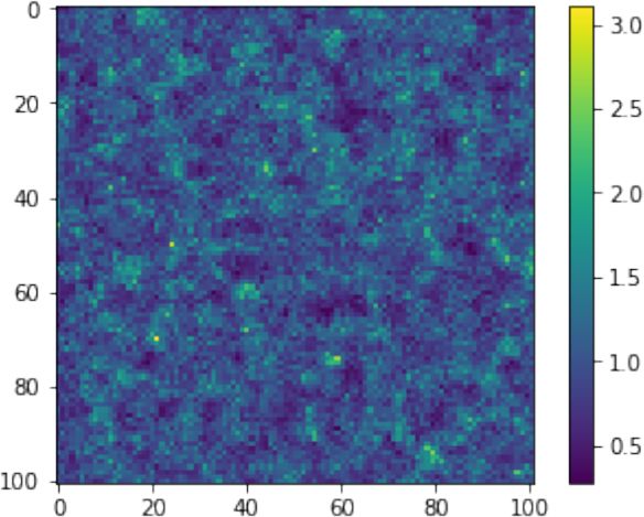
In addition, solar telescopes typically point at lower elevations than night-time telescopes, which have the
luxury of observing targets when they are higher in the sky. If the wavefront sensors (WFSs) are conjugate to
the ground (i.e., in the pupil plane), then the propagation between the high altitude DM and the ground leads
to a pupil distortion. A distorted pupil leads to a change in registration between the WFSs and the DM. If the
interactuator spacing is matched to the size of the subaperture, a pupil distortion of half a subaperture leads to
an unstable loop, because an actuator poke will be incorrectly reconstructed as originating from a neighboring
actuator.
The distorting effect of the high-altitude DMs on the exit pupil in MCAO was first noticed by von der Lühe
while observing rapid intensity fluctuations in the MCAO corrected image plane at the VTT.8 Later, it was
realized that the ever changing shape of the high-altitude DM that continuously changes the registration between
the pupil DM and the WFS could potentially pose a challenge to MCAO control. In a 2010 paper, Schmidt et al.
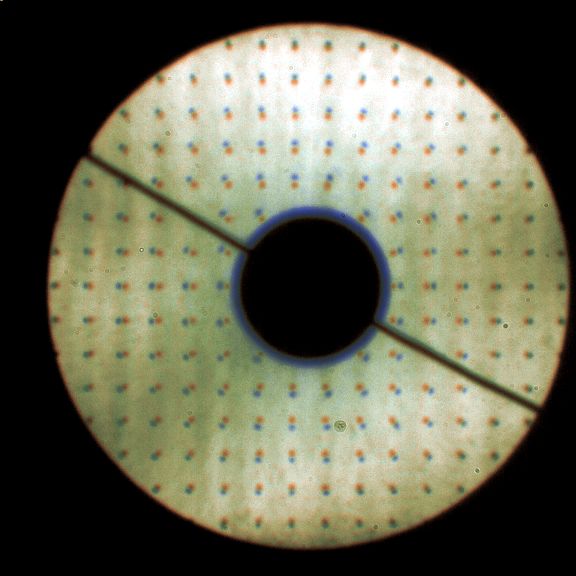
demonstrated the dynamic misregistration using ray tracing and experimentally. Figure 1 illustrates the pupil
distortion and the associated dynamic misregistration of the the Gregor MCAO system by poking the central
actuator of the high altitude DM.9
Figure 1: Photographic illustration of pupil distortion: the same grid pattern is shown with the DMs flat and
with a 400 nm poke of the central actuator on high-altitude DM (left). The region corresponds to an area
spanning approximately 3 × 3 actuators marked with a cross (right).9
In the second generation of solar MCAO systems at Gregor and Clear at the Goode Solar Telescope, it was a
goal to mitigate the misregistration issue. In the Gregor system, a high-order on-axis WFS was placed between
the pupil DM and the high-altitude DMs, and a low-order multi-directional WFS was placed behind all DMs.
The same scheme was available in Clear as one of six different WFS and DM concepts implemented. This control
strategy is stable and produced AO corrected images.6, 10, 11
In Section 2, we compare existing AO simulation and describe how they propagate the wavefront. To our
knowledge, there is no existing end-to-end Monte-Carlo simulation tool that models solar MCAO and reproduces
this effect. We considered three different ways to model the pupil distortion:
• Fresnel propagation
• Ray tracing (using the start point and the gradient of the ray to determine the end point)
• The irradiance transport equation along with the associated wavefront transport equation12
The quickest way to create a new simulation tool with the required properties was to adapt PROPER,13 an
optical propagation code based on Fresnel propagation (Section 3).
In this paper, we develop PropAO, the first AO simulation tool (to our knowledge) to model the effect of pupil
distortion. PropAO takes advantage of the optical propagation library PROPER and uses Fresnel propagation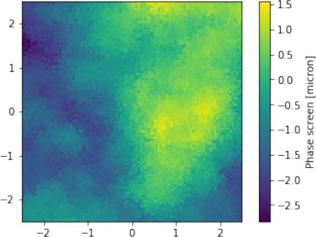
to propagate the amplitude and phase of an incoming wave through the atmosphere and the MCAO system.
The resulting wavefront is analyzed by the WFSs and also used to evaluate the corrected image quality. We are
able to reproduce the problem of pupil distortion and test novel non-linear reconstruction strategies that take
the distortion into account and produce well-corrected wide field images.
   Existing AO systems use linear wavefront reconstruction techniques, where the estimates wavefront is a linear
combination of the measured wavefront derivatives. In Section 4, we propose new reconstructors to combat
the pupil distortion problem. Simulation results using a toy MCAO problem are presented in Section 5 and
conclusions are drawn in Section 6.
   The motivation for this work is the design of the 4.2 m diameter European Solar Telescope.14, 15 The current
design has a very ambitious 4000 ×4000 AO-corrected science field of view. In order to deliver near diffraction-
limited performance at visible wavelengths over such a wide field of view, an MCAO system with three to five
DMs is under consideration. The ability to model the pupil distortion is essential to the success of the EST
project. The PropAO tool and the results of this work are also applicable to other solar and night-time astronomy
MCAO systems.

                                2. EXISTING SIMULATION CODES
In this section, we describe publicly available and well-documented end-to-end simulation codes. We evaluate
them on their suitability to model the pupil distortion of a solar MCAO system and find that none of these codes
can be used to model the pupil distortion.

2.1 DASP
The Durham Adaptive optics Simulation Platform (DASP) is an open-source configurable AO simulation en-
vironment written in Python.16, 17 DASP offers support for tomographic reconstructors and pseudo-open loop
control, so it is well suited for MCAO simulations. The turbulence propagation is performed either by simple
integration of the wavefront along the line of sight or using Fresnel propagation. Only the former option is
currently available for propagation through the DM to the WFSs. Implementing this using Fresnel propagation,
while not a lot of work, is not in the pipeline.18

2.2 YAO
A full-featured end-to-end Monte-Carlo simulation tool, known as yorick adaptive optics (YAO) and written
by Francois Rigaut, is used extensively in the AO community.19, 20 The wavefront propagation is performed by
summing the wavefront through each atmospheric layer or DM surface in the direction of each WFS or science
target. Fresnel propagation is not implemented. The pupil distortions are not modeled.

2.3 OOMAO
OOMAO is a Matlab based AO simulation tool that is highly configurable. The wavefront propagation is
performed in the same way as YAO, so the pupil distortion is not modeled, either.

2.4 CAOS
The Software Package CAOS is a subset of the CAOS Problem-Solving Environment and consists of an IDL
based AO simulations tool.21, 22 It uses linear wavefront propagation to calculate the wavefronts. It was claimed
in 2005 that “a Fresnel module for atmospheric turbulence has been written and will be part of a forthcoming
release.”24 This claim is still true today! Work on Fresnel propagation through turbulence was paused, has
recently restarted but is not yet ready for release.23 It is possible to also implement Fresnel propagation between
DMs at different conjugate altitudes, but this functionality is not planned.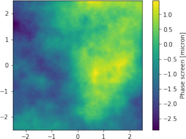
2.5 CEO
CEO (an acronym for Cuda Engined Optics) is a simulation tool written for the Giant Magellan Telescope.25, 26
This open-source software applies ray tracing in CUDA and has a Python interface. It has the capability to
apply ray tracing through the atmosphere and the telescope, but not through an AO system. This capability
would be needed to model the pupil distortions.
   Figure 2 shows how the wavefront propagation leads to variations in wavefront and amplitude using ray
tracing in CEO.

    Figure 2: Phase before propagation (left) and phase (center) and amplitude (right) after propagation.

3. PROPAO: AN EXTENSION TO THE PROPER OPTICAL PROPAGATION TOOL
The PROPER optical propagation code, available in IDL, Matlab and Python, is a library of routines for optical
propagation.13, 27 PROPER uses full Fresnel propagation at every step and is suitable for modeling the complex
amplitude of a wave propagating through the atmosphere and an MCAO system. There is support for pupil
stops, DMs, and point-spread function (PSF) generation. An example of Fresnel propagation using PROPER is
shown in Figure 3, where a Kolmogorov phase screen is propagated 20 km in broadband light over a the range
of 400 nm to 800 nm nm. The amplitude and the phase evolve as the wave propagates.
    In this section, we show how we extend the functionality of PROPER into an end-to-end simulation tool.
PropAO uses the Python 3 version of the PROPER optical propagation tool as a starting point and adds new
features missing in PROPER, such as atmospheric turbulence and WFSs, in order to create an end-to-end MCAO
simulation tool. As will become evident, the development process consisted a tool that mimicked the behavior
of YAO as closely as possible in order to quickly and efficiently debug and verify the new code using a simple
single conjugate AO system. Once we were confident in the results, the simulation was extended to an MCAO
with multiple DMs and WFSs.

3.1 Atmospheric turbulence
PROPER has the capability of inserting amplitude or phase screens anywhere in the optical train, but no function
to create Kolmogorov phase screens. Atmospheric phase screens were generated using YAO to avoid writing code
unnecessarily, and to make it easier to compare the results between the two codes. The optical propagation begins
at the top of the atmosphere, where the first atmospheric phase screen is inserted. The complex amplitude is
propagated to the next atmospheric phase screen, where the phase corresponding to the second atmospheric
phase screen is added. This procedure is repeated until we reach the top of the telescope.

3.2 Telescope
The telescope is modeled as an ideal telescope. The complex amplitude of the incoming wave is multiplied by a
circular function representing the exit pupil of the telescope by calling a PROPER function. In the future, we
could include a realistic optical model of the telescope.
Figure 3: Initial amplitude and phase (top) and final amplitude and phase (bottom) following a 20 km propagation using the PROPER code. 3.3 Deformable mirrors The first DM is conjugate to the pupil, so no propagation from the telescope exit pupil is required. The complex amplitude is multiplied by the phase induced by the DM and the wave is propagated to the first altitude DM. This process was repeated for all DMs. Finally, the wave is progated back to the pupil plane, where the wavefront sensors (WFSs) and the science instruments are situated. The functions in PROPER used to mode DMs were initially used. However, two limitations drove us to write our own DM module: flexibility and speed. The DM influence functions in PROPER are hard coded to a particular function that is loaded as a FITS file. We wanted to be able to specify the same influence functions as YAO initially, and then to be able to use the influence functions corresponding to a real DM. The DM implementation in PROPER was also prohibitively slow. The new implementation for the DMs is as follows. First, the user can define an actuator influence function or use one of the pre-programmed ones. The options include the sinc interpolator, the bilinear intepolator, an approximation to the measured influence function of a Xinetics actuator, and the same function that is programmed in YAO. The two-dimensional actuator commands are convolved with the influence function. The convolution takes place as a multiplication in the Fourier domain using FFTs. 3.4 Wavefront sensors There are no WFSs in PROPER. Shack-Hartmann WFSs were implemented in the following manner. The complex amplitude at the pupil plane is subdivided by the lenslet array and each subaperture is propagated onto the pupil plane to form an image. The centroid of the image on each subaperture is computed and recorded.
3.5 Wavefront reconstruction and control
The main purpose of the tool is to investigate wavefront reconstruction and control strategies. The tool supports
closed-loop and open-loop (where the WFSs do not see the DMs) modes as well as pseudo open-loop control, as
described in Section 4.

3.6 Science instrument
The science instrument is modeled as an imager which takes an image of a point source and uses this image to
estimate the Strehl ratio at the science wavelength(s). There is the option of including a pupil stop in the science
camera.

3.7 Use of GPUs with the CuPY library
Following the completion of the first operational version PropAO, it was evident from modeling a 1 m diameter
telescope that the simulations could not be scaled to a 4.2 m diameter telescope like the European Solar Telescope
due to the computational load. Since most of the computations consist of FFTs and matrix multiplications,
PropAO is an ideal candidate for the use of Graphical Processing Units (GPUs). The CuPY library is a
Python library that uses CUDA acceleration for the heavy numerical computations.28 It is almost a like-to-like
replacement for the NumPY library, which is used in PROPER. By making a small number of changes (fewer
than ten different lines of code), we were able to convert the computations in PropAO from CPU to GPU. The
simulation time using an off-the-shelf laptop (Dell Precision 7710 with an NVIDIA Quadro M4000M GPU on
a laptop) decreased by a factor of 100! As an example, a 3 DM system on a 4 m telescope with 5 32 × 32
subaperture WFSs runs at 2.5 iterations/second.

                   4. WAVEFRONT RECONSTRUCTION AND CONTROL
In this section, we describe a number of different approaches to the problem of wavefront reconstruction and
control, which are subsequently evaluated using PropAO simulations.

4.1 Closed-loop control with regularized least-squares reconstructor
The standard closed-loop reconstructor is what is used on almost all AO systems. An interaction matrix is
created by poking the actuators one by one. The reconstructor is computed as a regularized inverse of the
interaction matrix, either using a singular value decomposition, a regularized least-squares inversion or a modal
basis set. We use the regularized least-squares reconstructor, R:
                                               −1
                                     R = (H T Cnn H + αCφ−1 + P )−1 H T Cnn
                                                                         −1
                                                                                                                (1)

where H is the interaction matrix, P is a matrix that penalizes piston for each DM, Cnn is the noise covariance
matrix, Cφ is the covariance matrix of the uncorrected turbulence and α is a regularization constant. Figure
4 plots the interaction matrix, covariance matrix and piston penalization matrix for a 3 DM, 5 WFS MCAO
system. The noise covariance matrix is simply a diagonal matrix.

Figure 4: Interaction matrix (left), covariance matrix (center) and piston penalization matrix (rigth) for a 3 DM,
5 WFS system.
The wavefront residual, u, is given by the matrix multiplication of the reconstructor, R, and the centroids, s:
u = Rs (2)
A leaky integrator with leak l=0.01 loop gain k=0.6 is used to update the actuator commands, a at time n:
a[n] = (1 − l)a[n − 1] + ku[n]. (3)
This reconstruction and control approach can lead to instabilities because the high altitude DMs will cause a
shift in the registration between the actuators of the lower altitude DM and the WFS lenslets.
4.2 Closed-loop control with iterative interaction matrix and regularized least-squares
reconstructor
The interaction matrix is calculated by poking actuators one by one away from their nominal positions and
measuring the centroids. However, the effect of each actuator on the WFS depends on the actuator commands of
the mirrors that follow it. For example, the effect that the ground-layer DM has on the WFS centroids depends
on the shape of the mid- and high-altitude DMs. In this control strategy, we calculate the interaction matrix
iteratively by poking actuators referenced to the current DM commands. Each time the interaction matrix is
calculate (once every ten iterations in the simulations presented in this paper), the reconstructor is recomputed.
4.3 Pseudo open-loop control with regularized least-squares reconstructor
The reconstructor in Eq. (1) can be used in pseudo open-loop control. Pseudo-open loop control uses the
open-loop centroids, s − Ha to calculate the residuals:
u = R(s + Ha) − a
u = Rs + (RH − I)a (4)
where I is the identity matrix.
4.4 Non-linear pseudo open-loop control with regularized least-squares reconstructor
The pseudo open-loop control described in Section 4.3 relies on a linear relationship between the actuator
commands and the centroids to compute the open-loop centroids. For strong turbulence, this relationship
does not hold due to the pupil distortion effect. A more accurate way to compute the open-loop centroids
is to propagate a wave from the top of the telescope through to the WFSs and measure the centroids. This
propagation takes place once per iteration.
4.5 Separate control of ground-layer DM and high-altitude DMs
In some solar MCAO systems, a high-order on-axis WFS is used to control the ground-layer DM, while lower-
order off-axis WFSs are used to drive the mid- and high-altitude DMs.10 The on-axis WFS does not see the
other DMs, so the registration between the WFS and the ground-layer DM is not affected by the other DMs.
Here, the optical setup is different, not just the control law!
5. SIMULATIONS
Simulations were run using new simulation tool and compared with the same simulations run in YAO in order
to understand the effects of Fresnel propagation through the atmosphere and AO system.5.1 Simulation parameters
The simulations were run using a 1 m diameter telescope with no central obscuration. In all cases, there are 8 × 8
subapertures across the pupil. Two different atmospheric profiles are used, one with 70% of the turbulence near
the ground (Profile 1) and another one with 90% (Profile 2). The turbulence parameters are tabulated in Table
2.
Elevatiion (m) 0 1000 2000 4000 8000 16000
Profile 1 Turbulence fraction 0.55 0.15 0.05 0.06 0.07 0.12
Profile 2 Turbulence fraction 0.63 0.25 0.02 0.02 0.03 0.05
Wind speed (m s−1 ) 5.6 6.25 7.57 13.31 19.06 12.14
Wind direction (°) 190 270 350 17 29 66
Table 2: Turbulence profiles used in the simulations.
The outer scale of turbulence used in the simulations is a few meters, which is not realistic. This occurs
because the phase screens are periodic in order to avoid issues with discontinuities when propagating with the
Fast Fourier Transform (FFT). The effect of the outer scale on AO-corrected performance is expected to be
small, but needs to be considered.
5.2 Seeing-limited simulations
Simulations were run with no correction as a sanity check, and compared with a YAO simulation using the same
parameters. There were 3000 iterations with a 10 ms exposure time for a total integration time of 30 s. There is
excellent consistency between the YAO and the PropAO results (Table 3), which is not suprising since the same
turbulence phase screens are used. The on-axis Strehl ratio at 500 nm is used as the science metric.
Profile 1 Profile 2
Elev. r0 = 8 cm r0 = 15 cm r0 = 25 cm r0 = 8 cm r0 = 15 cm r0 = 25 cm
YAO 20° 0.0020 0.0061 0.0160 0.0020 0.0062 0.0164
PropAO 20° 0.0018 0.0063 0.0179 0.0018 0.0063 0.0176
YAO 45° 0.0043 0.0145 0.0394 0.0044 0.0146 0.0405
PropAO 45° 0.0042 0.0156 0.0432 0.0043 0.0153 0.0415
YAO 90° 0.0067 0.0232 0.0607 0.0063 0.0221 0.0593
PropAO 90° 0.0067 0.0232 0.0607 0.0063 0.0221 0.0593
Table 3: Strehl ratio at 500 nm from YAO and PropAO simulations of uncorrected turbulence.
5.3 Single conjugate adaptive optics simulations
A simple single conjugate adaptive optics (SCAO) system was simulated using both codes. A ground-layer DM
with 9 × 9 actuators across the pupil in the so-called Fried configuration was used. The WFS exposure time was
1 ms, and 1000 iterations were run for a total simulation time of 1 s. All of the simulations in this section are
performed using pseudo open-loop control with an optimized value of α in the least-squares inversion of Eq. (1).
The turbulence was moved to the ground in order to avoid scintillation effects, which are not modeled in YAO.
The results are tabulated in Table 4.Profile 1 Profile 2
Elev. r0 = 8 cm r0 = 15 cm r0 = 25 cm r0 = 8 cm r0 = 15 cm r0 = 25 cm
YAO 20° 0.093 0.443 0.706 0.098 0.452 0.712
PropAO 20° 0.089 0.421 0.690 0.102 0.442 0.703
YAO 45° 0.321 0.673 0.844 0.321 0.674 0.845
PropAO 45° 0.305 0.657 0.832 0.325 0.672 0.840
YAO 90° 0.435 0.745 0.882 0.437 0.747 0.882
PropAO 90° 0.431 0.741 0.876 0.451 0.754 0.882
Table 4: Strehl ratio at 500 nm from YAO and PropAO simulations of an SCAO system with all of the turbulence
near the ground.
The theoretical decrease in Strehl ratio, S due to scintillation is given by the Maréchal approximation for
sufficiently small amplitude vatiations:
S = exp[−σχ2 ] (5)
where the scintillation is calculated as29
Z
σχ2 = 0.5631k 7/6 sec11/6 (ζ) dzCn2 (z)z 5/6 . (6)
The symbol ζ represents the zenith angle, and k is the wave number, 2π/λ.
PropAO simulations were repeated with the turbulence phase screens at their nominal value, and the decrease
in Strehl ratio was compared to the expected decrease in Strehl due to scintillation (Table 5). In general, both
sets of results show the same trends, but the fit is not perfect. Part of the reason is that the scintillation also has
an effect on the WFS, so the Strehl ratio is worse than predicted when the scintillation is strong. The results at
an elevation of 20° are omitted because the Maréchal approximation does not hold.
Profile 1 Profile 2
Elev. r0 = 8 cm r0 = 15 cm r0 = 25 cm r0 = 8 cm r0 = 15 cm r0 = 25 cm
Analytic 45° 0.891 0.960 0.983 0.942 0.979 0.991
PropAO 45° 0.790 0.951 0.994 0.898 0.987 0.998
Analytic 90° 0.941 0.978 0.991 0.969 0.989 0.995
PropAO 90° 0.929 0.991 0.998 0.970 0.996 0.999
Table 5: Strehl ratio at 500 nm from YAO and PropAO simulations of an SCAO system with all of the turbulence
near the ground.
5.4 Multiconjugate adaptive optics simulations
Simulations were run for a toy 3-DM MCAO system using the same 1 m telescope. The DM parameters are as
described in Table 6.
DM number Altitude Interactuator spacing Actuators across pupil
0 0m 125 mm 9×9
1 5000 m 250 mm 7×7
2 12 000 m 375 mm 6×6
Table 6: Description of the DMs used in the MCAO simulations.
There are five identical WFSs with 8 × 8 subapertures. The guide stars are modeled as point sources located
at [000 , 000 ], [±500 , ±500 ]. The science field of view is a 1000 × 1000 square. The results from the YAO simulationsusing pseudo open-loop control are displayed in Table 7. All of these YAO simulations exhibited loop stability
and improved the image quality; this is not surprising, because YAO does not model the pupil distortion. It is
clear that some configurations, such as observing at an elevation of 20° in anything but the best seeing, are not
really suitable for wide-field MCAO correction.
Profile 1 Profile 2
Elev. r0 = 8 cm r0 = 15 cm r0 = 25 cm r0 = 8 cm r0 = 15 cm r0 = 25 cm
20° 0.005±0.001 0.037±0.016 0.152±0.058 0.008±0.002 0.092±0.032 0.316±0.065
45° 0.088±0.023 0.417±0.040 0.687±0.028 0.189±0.021 0.548±0.022 0.773±0.013
90° 0.268±0.017 0.629±0.015 0.820±0.008 0.361±0.011 0.699±0.008 0.858±0.004
Table 7: Strehl ratio at 500 nm from MCAO simulations using YAO with psedo open-loop control.
These simulations were repeated in PropAO using a variety of reconstruction strategies, described in Section
4:
• Regularized least-squares reconstructor operating in closed-loop (CL)
• Regularized least-squares reconstructor with an iterative interaction matrix operating in closed-loop (Iter
CL)
• Regularized least-squares reconstructor operating in pseudo open-loop (POLC)
• Regularized least-squares reconstructor with non-linear pseudo open-loop (NL POLC)
The performance achieved was very sensitive to the level of regularization (the value of the α parameter)
used in the reconstructor, with the regularization adjusted for each simulation in order to maximize the Strehl
ratio. For strong turbulence cases, a high level of regularization was needed to maintain loop stability.
Profile 1 Profile 2
Elev. r0 = 8 cm r0 = 15 cm r0 = 25 cm r0 = 8 cm r0 = 15 cm r0 = 25 cm
CL 20° — 0.045±0.012 0.206±0.050 — 0.119±0.034 0.385±0.047
Iter CL 20° 0.005±0.001 0.046±0.021 0.206±0.048 0.008±0.002 0.119±0.031 0.375±0.041
POLC 20° — 0.048±0.019 0.206±0.043 — 0.128±0.029 0.384±0.038
NL POLC 20° — 0.046±0.016 0.200±0.042 — 0.116±0.025 0.367±0.038
CL 45° 0.064±0.012 0.402±0.035 0.663±0.024 0.142±9.014 0.536±0.021 0.754±0.013
Iter CL 45° 0.068±0.015 0.388±0.035 0.658±0.025 0.142±0.010 0.520±0.022 0.729±0.015
POLC 45° 0.075±0.015 0.419±0.035 0.675±0.024 0.182±0.020 0.550±0.021 0.763±0.021
NL POLC 45° 0.075±0.017 0.397±0.034 0.660±0.024 0.152±0.017 0.523±0.021 0.747±0.013
CL 90° 0.226±0.014 0.587±0.012 0.783±0.007 0.267±0.012 0.670±0.009 0.831±0.006
Iter CL 90° 0.194±0.012 0.575±0.012 0.784±0.007 0.288±0.010 0.662±0.008 0.816±0.008
POLC 90° 0.249±0.015 0.618±0.013 0.806±0.007 0.358±0.011 0.696±0.008 0.849±0.005
NL POLC 90° 0.224±0.014 0.600±0.013 0.797±0.008 0.318±0.011 0.673±0.008 0.838±0.005
Table 8: Strehl ratio at 500 nm from MCAO simulations using PropAO with varying reconstruction and control
strategies.
The results in Table 8 shows that all of the methods could close the loop successfully, except in the worst
case where the turbulence was strong and the elevation was low. The key to loop stability was a high level of
regularization, but this limits the attainable atmospheric correction.
The best control strategy is to use linear pseudo open-loop control. The non-linear control strategies did not
improve the performance across the board and often made things worse.5.5 Multiconjugate adaptive optics simulations with decoupled DM control
The simulation is run using the same DM configuration is used, but two sets of WFSs are used:
• a pick-off after the ground-layer DM that feeds an on-axis WFS with 8x8 subapertures across the pupil.
• A second pick-off following the three DMs feeds the four off-axis WFSs, which have 4x4 subapertures across
the pupil.
The correction of the ground-layer DM is decoupled from the high-altitude DMs, as described in Schmidt et al.6
Simulations run using YAO and PropAO show consistent results, with the PropAO values lower than the
YAO results mostly due to scintillation (Table 9). The Strehl ratios are much lower than those obtained in
Section 5.4. The decoupled DM control strategy has lower performance because the on-axis wavefront is not the
same as the wavefront at the ground. This strategy should not be used.
Profile 1 Profile 2
Elev. r0 = 8 cm r0 = 15 cm r0 = 25 cm r0 = 8 cm r0 = 15 cm r0 = 25 cm
YAO 20° 0.004±0.001 0.025±0.006 0.101±0.022 0.007±0.001 0.057±0.012 0.230±0.034
PropAO 20° 0.001±0.000 0.018±0.004 0.086±0.033 0.001±0.000 0.038±0.011 0.187±0.045
YAO 45° 0.033±0.019 0.260±0.049 0.555±0.042 0.101±0.022 0.436±0.030 0.700±0.020
PropAO 45° 0.019±0.005 0.210±0.032 0.516±0.033 0.063±0.011 0.379±0.025 0.660±0.019
YAO 90° 0.097±0.028 0.421±0.040 0.688±0.027 0.217±0.026 0.581±0.023 0.793±0.013
PropAO 90° 0.056±0.012 0.367±0.029 0.660±0.022 0.160±0.015 0.544±0.022 0.770±0.021
Table 9: Strehl ratio at 500 nm from YAO and PropAO simulations using MCAO with decoupled control.
6. CONCLUSION
A major stumbling block in attaining diffraction-limited images over a wide field using MCAO on solar telescopes
is the dynamic change in registration between the pupil DMs and the WFSs. While this phenomenon is well
understood, a simulation tool to study this problem and test potential solutions have not been available until
now.
In this paper, we present a new AO simulation tool, PropAO, based on the PROPER optical propagation
tool which propagates waves from plane to plane using Fresnel propagation. The Python version of the PROPER
tool has been extended by adding features needed for an end-to-end MCAO simulation and has been modified
to run on GPUs using the CuPY library, considering the large number of Fresnel propagations required. The
simulation tool has been extensively tested by comparing outputs from simple cases to the open-source Monte-
Carlo simulation tool, YAO, with excellent agreement between the codes.
The effect of the pupil distortion on the registration between the DMs and the WFSs is readily seen in
PropAO simulations. While the ultimate solution to wavefront reconstruction in the presence of pupil distortion
remains elusive, it can be partially mitigated by using using a heavily regularized least-squares reconstructor in
conjunction with pseudo open-loop control. This leads to a stable reconstruction for a wide range of observing
conditions, and much better performance than what is attained when decoupling the control of the pupil DM
and the high altitude DM using dedicated WFSs for each one.
PropAO will be used to simulate the MCAO system for the EST and to test potential implementations of
wavefront control. It can also be used for any MCAO system for solar or night-time astronomy.Acknowledgments
This work was supported by the EST Project Office, funded by the Canary Island Government (file SD 17/01)
under a direct grant awarded to EST on ground of public interest.
We extend our gratitude to Dirk Schmidt (NSO), who has been battling the dynamic misregistration problem
for many years, for his advice and help with the manuscript. The authors would also like to thank John Krist
(JPL) for advice on the use of PROPER and Rodolphe Conan (GMT) for the suggestion to use the CuPY library
in place of the NumPY library.
REFERENCES
[1] Marchetti, Enrico, et al. “MAD: the ESO multiconjugate adaptive optics demonstrator.” Adaptive Optical
System Technologies II. Vol. 4839. International Society for Optics and Photonics, 2003.
[2] Rigaut, François, et al. “Gemini multiconjugate adaptive optics system review–I. Design, trade-offs and
integration.” Monthly Notices of the Royal Astronomical Society 437.3 (2013): 2361-2375.
[3] Neichel, Benoit, et al. “Gemini multiconjugate adaptive optics system review–II. Commissioning, operation
and overall performance.” Monthly Notices of the Royal Astronomical Society 440.2 (2014): 1002-1019.
[4] Thomas Berkefeld et al, “Results of the multi-conjugate adaptive optics system at the German solar telescope,
Tenerife,” Proc. SPIE 5903, 59030O (2005).
[5] Thomas Berkefeld et al, “Multi-conjugate solar adaptive optics with the VTT and GREGOR,” Advances in
Adaptive Optics II. Vol. 6272. International Society for Optics and Photonics, 2006.
[6] Schmidt, Dirk, et al. “Clear widens the field for observations of the Sun with multi-conjugate adaptive optics.”
Astronomy & Astrophysics 597 (2017): L8.
[7] Schmidt, Dirk, Thomas Berkefeld, and Frank Heidecke. “The 2012 status of the MCAO testbed for the
GREGOR solar telescope,” Adaptive Optics Systems III. Vol. 8447. International Society for Optics and
Photonics, 2012.
[8] von der Luhe, Oskar FH. ”Photometric stability of multiconjugate adaptive optics.” Advancements in Adap-
tive Optics. Vol. 5490. International Society for Optics and Photonics, 2004.
[9] Schmidt, Dirk, et al. “Latest achievements of the MCAO testbed for the GREGOR Solar Telescope.” Adaptive
Optics Systems II. Vol. 7736. International Society for Optics and Photonics, 2010.
[10] Schmidt, Dirk, et al., “Progress in multi-conjugate adaptive optics at Big Bear Solar Observatory.” Adaptive
Optics Systems V. Vol. 9909. International Society for Optics and Photonics, 2016.
[11] D. Schmidt et al., “GREGOR MCAO looking at the Sun,” Proc. SPIE 9148, 91481T (2014).
[12] M. R. Teague, “Deterministic phase retrieval: a Green’s function solution”, J. Opt. Soc. Am. 73, 1434-1441
(1983).
[13] Krist, J., “PROPER: an optical propagation library for IDL,” Proc. SPIE, 6675, 66750P (2007).
[14] Montoya, L et al. “MCAO numerical simulations for EST: analysis and parameter optimization,” Adaptive
Optics for Extremely Large Telescopes 4–Conference Proceedings. Vol. 1. No. 1. 2015.
[15] Berkefeld, Thomas. “Status of the preparatory work for the 4m European Solar Telescope.” Adaptive Optics
Systems VI. Vol. 10703. International Society for Optics and Photonics, 2018.
[16] Basden, A. G., et al. “The Durham Adaptive Optics Simulation Platform (DASP): Current status.” Soft-
wareX 7 (2018): 63-69.
[17] https://github.com/agb32/dasp
[18] A. Basden, personal communications, email dated 15 July 2019.
[19] F. Rigaut and M. van Dam,“Simulating Astronomical Adaptive Optics Systems Using Yao,” AO4ELT3
(2013).
[20] https://github.com/frigaut/yao
[21] M. Carbillet and A. La Camera, “The CAOS Problem-Solving Environment: tools for AO numerical mod-
elling and post-AO deconvolution,”AO4ELT5, DOI:10.26698/AO4ELT5.0059 (2017).
[22] https://www-n.oca.eu/caos/
[23] Carbillet, M., personal communications, emails dated 17 Nov 2020.[24] Carbillet, M., et al. “Modelling astronomical adaptive optics-I. The software package CAOS.” Monthly Notices of the Royal Astronomical Society 356.4 (2005): 1263-1275. [25] Conan, Rod, et al., “The GMT Dynamic Optical Simulation.” Adaptive Optics for Extremely Large Tele- scopes 4–Conference Proceedings. Vol. 1. No. 1. 2015. [26] https://github.com/rconan/CEO [27] http://proper-library.sourceforge.net/ [28] https://cupy.dev/ [29] R. Sasiela, Electromagnetic Wave Propagation in Turbulence, p111, 2nd edition (2007).
You can also read