Optimizing the assortment planning of highly differentiated products with

Master of Science in Industrial Engineering
 June 2022

 Optimizing the assortment planning of
 highly differentiated products with
demand and location complexity in Europe
 A case of the e-commerce cosmetic industry

 Rania Shalan and Rim Abdul-Rahman

 Faculty of Industrial Economics, Blekinge Institute of Technology, 371 79 Karlskrona,
 Sweden

This thesis is submitted to the Faculty of Industrial Economics at Blekinge Institute of Technology
in partial fulfilment of the requirements for the degree of Master of Science in Industrial Economics
Engineering. The thesis is equivalent to 20 weeks of full time studies.

 The authors declare that they are the sole authors of this thesis and that they have not used any
sources other than those listed in the bibliography and identified as references. They further declare that
they have not submitted this thesis at any other institution to obtain a degree.

 Contact Information:
 Author(s):
 Rania Shalan
 E-mail: rash17@student.bth.se

 Rim Abdul-Rahman
 E-mail: riab17@student.bth.se

 University supervisor:
 Philippe Rouchy
 Industrial Economics

 Faculty of Industrial Economics Internet : www.bth.se
 Blekinge Institute of Technology Phone : +46 455 38 50 00
 SE-371 79 Karlskrona, Sweden Fax : +46 455 38 50 57
 ii

ABSTRACT
The cosmetic industry is characterized by having the ability to offer a wide range of differentiated
products. This leads in turn retailers to make strategic decisions regarding assortment planning. It
means choosing the right breadth and depth of products that should be allocated to a distribution
center. This is essential to the ability to answer the needs of their customers. Besides the range of
products retailers also face the choice of the optimal location of the distribution center. Both the range
of carefully chosen products and agglomeration economies affect efficiency, customer satisfaction as
well as transportation delays and costs. Therefore, in this research, we have developed a framework to
optimize both the ranges of products and agglomeration economies. To do this study, we have
collaborated with LYKO AB, a firm within the cosmetics industry offering highly differentiated
products with e-commerce solutions. We frame their problem by creating a three-step optimization
solution. It is combined with a demand module, optimization module, and localization module. The
result showed that 36 products within the selected subset had a high demand,10 out of these products
further maximized the profit of the firm. The localization module showed that among the four
considered countries in Europe (Germany, Netherlands, Poland, and Austria) the optimal geographical
location to locate the warehouse was Germany. This result was based on logistic decisions such as
customer population, best distance, and level of competition. In conclusion, to be able to optimize the
assortment planning of highly differentiated products to maximize the profit based on localization and
customer demand complexity one can use a three-step optimization solution.

 Keywords: Optimization, assortment planning, localization, demand model, TOPSIS-model

 iii

SAMMANFATTNING
Den kosmetiska industrin är karakteriserad genom att ha förmågan att erbjuda ett brett utbud av
differentierade produkter. Detta leder i sin tur till återförsäljare att fatta strategiska beslut om
sortimentsplanering. Detta innebär att välja rätt bredd och djup av produkter som ska allokeras till ett
distributionscenter. Detta är viktigt för förmågan att svara på kundbehovet. Förutom produktutbudet står
återförsäljarna också inför valet av den optimala placeringen av distributionscentret. Både
produktutbudet och agglomerationsekonomi påverkar effektiviteten, kundnöjdheten såväl som
transportförseningar och kostnader. Därför har vi i denna forskning utvecklat ett ramverk för att
optimera både produktutbudet och agglomerationsekonomi. För att göra denna studie har vi samarbetat
med LYKO AB, ett företag inom den kosmetiska industrin som erbjuder högt differentierade produkter
med e-handel lösningar. Vi sätter samman problemen genom att skapa en trestegsoptimeringslösning
bestående av en efterfrågamodul, en optimeringsmodul och en lokaliseringsmodul. Resultatet visade att
36 produkter bland de utvalda produkterna hade en hög efterfrågan, 10 av dessa produkter maximerade
företagets vinst ytterligare. Lokaliseringsmodulen visade att mellan de fyra övervägda länderna i Europa
(Tyskland, Nederländerna, Polen och Österrike) var den optimala geografiska platsen för att lokalisera
lagret i Tyskland. Detta resultat baserades på logistiska beslut som kundpopulation, bästa avstånd och
konkurrensnivå. Sammanfattningsvis, för att kunna optimera sortimentsplaneringen för högt
differentierade produkter för att maximera vinsten baserat på plats och kundefterfrågans komplexitet
kan man använda en trestegsoptimeringslösning.

 Nyckelord: Optimering, sortimentplanering, lokalisering, efterfråga modell, TOPSIS-modell

 iv

Acknowledgments
First, we would like to thank our supervisor Philippe Rouchy at Blekinge Institute of Technology, for
his support and feedback. It has improved our thesis enormously. We would also like to thank our
supervisors Ellinor Belin and Daniel Wikar at LYKO AB for making it possible for us to take on this
thesis project and for the help they have provided.

Finally, we want to thank the department of industrial economics and Blekinge Institute of
Technology for the five years of education and experience.

Thank you!
Rim Abdul-Rahman
Rania Shalan

Blekinge Institute of Technology
M. Sc. in Industrial Management and Engineering, 300 ECTS
Master Thesis, 30 ECTS
2022-06-05

 v

LIST OF CONTENT
 ABSTRACT ................................................................................................................................................ III

 SAMMANFATTNING ............................................................................................................................... IV

 1 INTRODUCTION ............................................................................................................................... 6
 1.1 BACKGROUND ............................................................................................................................... 6
 1.1.1 The Cosmetic Industry .............................................................................................................. 7
 1.1.2 Assortment planning ................................................................................................................. 8
 1.1.3 Localizing warehouses ............................................................................................................. 9
 1.1.4 Optimization models ................................................................................................................. 9
 1.2 THE SCOPE OF THE RESEARCH AND THE PROBLEM FORMULATION ............................................... 10
 1.3 THE THESIS OUTLINE ................................................................................................................... 10
 2 LITERATURE REVIEW ................................................................................................................. 12
 2.1 ASSORTMENT PLANNING AND DEMAND MODELS ......................................................................... 12
 2.2 OPTIMIZATION OF WAREHOUSE LOCATION PROBLEM .................................................................. 14
 3 METHOD OPTIMIZATION ........................................................................................................... 16
 3.1 PURPOSE AND RESEARCH QUESTION ............................................................................................ 16
 3.2 DATA COLLECTION...................................................................................................................... 16
 3.3 RETAIL WAREHOUSE LOCATION: THE OPTIMAL COMBINATION OF ASSORTMENT PLANNING, COST,
AND LOCATION .................................................................................................................................................. 17

 4 RESULTS AND ANALYSIS: OPTIMIZING DEMAND, PRODUCTS, AND LOCATION ..... 23
 4.1 THE PRODUCTS THAT ARE IN HIGH DEMAND - THE DEMAND MODEL ............................................ 23
 4.1.1 Interpretation of the demand model regarding the results ..................................................... 23
 4.2 THE PRODUCTS THAT MAXIMIZE PROFIT - THE OPTIMIZATION MODEL ......................................... 24
 4.2.1 Understanding the optimization model and what products that maximize the profit given the
 constraints 25
 4.3 THE OPTIMAL GEOGRAPHICAL SOLUTION FOR THE WAREHOUSE LOCATION ................................. 26
 4.3.1 Where to localize the warehouse – breaking down the localization model ............................ 31
 5 DISCUSSION ..................................................................................................................................... 33
 5.1 THE FIRST MODULE – SELECTING THE DEMAND MODEL ............................................................... 33
 5.1.1 Other discrete choice models ................................................................................................. 34
 5.2 THE THIRD MODULE – CONSIDERING THE SELECTION OF THE LOCALIZATION MODEL .................. 35
 5.2.1 Multiple criteria decision-making approaches ....................................................................... 36
 5.3 HOW OUR RESULTS DIFFER FROM THE EXISTING LITERATURE AND OUR CONTRIBUTION TO
RESEARCH .................................................................................................................................................... 36
 5.4 GENERALIZATION AND TRANSFERABILITY................................................................................... 37
 6 CONCLUSION .................................................................................................................................. 38
 6.1 FUTURE WORK ............................................................................................................................. 40
 REFERENCES ........................................................................................................................................... 41

 7 APPENDIX ........................................................................................................................................ 43

 vi

LIST OF FIGURES
Figure 1: Network of the cosmetic industry ............................................................................................ 7
Figure 2: General model of assortment planning and warehouse location............................................ 17
Figure 3: The MNL-model, input, and output ....................................................................................... 18
Figure 4: Optimization model, input, and output .................................................................................. 19
Figure 5: Localization model, input, and output ................................................................................... 20
Figure: 6 Step by step calculation framework of the TOPSIS model ................................................... 45
Figure 7: The input for the optimizer in Gurobi .................................................................................... 45
Figure 8: The result of the optimizer in Gurobi .................................................................................... 46

 Faculty of Industrial Economics, Blekinge Institute of Technology, 371 79 Karlskrona,
 Sweden

LIST OF TABLES
Table 1: List of variables and their description ..................................................................................... 20
Table 2: TOPSIS input model ............................................................................................................... 21
Table 3: Data of the result from the optimization model ...................................................................... 24
Table 4: MNL-regression of having Germany as a base outcome, comparing the demand of products
 that are selected to the assortment vs products that are not selected with different regions ......... 27
Table 5:MNL-regression of having Poland as a base outcome, comparing the demand of products that
 are selected to the assortment vs products that are not selected with different regions ................ 27
Table 6: MNL-regression of having the Netherlands as a base outcome, comparing the demand of
 products that are selected to the assortment vs products that are not selected with different regions
 ....................................................................................................................................................... 28
Table 7:MNL-regression of having Austria as a base outcome, comparing the demand of products that
 are selected to the assortment vs products that are not selected with different regions ................ 29
Table 8: Complied cross table of the results. Showing the MNL-regressions of customer purchases in
 different regions based on high vs low demand products ............................................................. 30
Table 9: Ranked list of the optimal solution for the geographical place, where 1 is the best and 4 is the
 least good solution ......................................................................................................................... 30
Table 10: Data of the result from the demand model ............................................................................ 43
Table 11: the distance in km between the center of every country is calculated................................... 44
Table 12: Calculation of steps 1-2 of the TOPSIS model ..................................................................... 44
Table 13: Calculation of step 3 of the TOPSIS model .......................................................................... 44
Table 14: Calculation of steps 4-5 of the TOPSIS model together with the final result ....................... 44
Table 15: Information for the calculation of the demand model ........................................................... 46

 3

LIST OF EQUATIONS
Equation 1: Utility function..................................................................................................................... 8
Equation 2: Mathematical demand model ............................................................................................. 18
Equation 3: Optimization function ........................................................................................................ 19
Equation 4: STATA MNL demand model ............................................................................................ 21

 4

Abbreviations

SKU Stock keeping units
TOPSIS The Technique for Order of Preference by Similarity to Ideal Solution
ELECTRE Elimination and Choice Expressing Reality
MNL-model Multinomial logit model
AHP Analytic Hierarchy Process
MCDM Multi-criteria decision making
IIA property Independence of irrelevant alternatives property
LoC Level of Competition
BD Best Distance
CP Customer Population

 5

1 INTRODUCTION
When considering online retailers (e-tailers) and assortment, the most significant and
challenging decision to make for firms is to choose the “right” assortment that will satisfy their
existing customers and attract new ones. However, to understand assortment planning and be
able to do some future research on the topic standardized terminologies need to be introduced.
Assortment planning is the process of retailers deciding on the width and the breadth to carry
in their product diffusion. The width refers to the different categories of products and the
breadth refers to the different product lines in each category, for example, different brands with
their different products (Cathy & Rafiq, 2006).
 Managers strive therefore to specify an assortment that maximizes sales subject to various
constraints, for example, a limited budget for product purchases or limited inventory space
(Kök, Fisher, & Vaidyanathan, 2015). This is to narrow down the selection of all available
products out there that are substitutions for each other and make sure that just the right products
with the highest popularity will be available in their assortment to satisfy their customers. Most
of the retailers that have many products in their assortment face the problem of product
assortment selection and in addition, how they should be chosen to a distribution center. This
becomes a complex problem since the retailers must choose the right assortment to ensure that
a complete order can be transported when a customer makes one (Li, 2007). However, no
solution explains how the assortment selection may fit all firms. For the constantly growing e-
tailer business, it becomes an even larger issue of customer information since the range of
products is populating the assortment.
 Another challenge associated with assortment planning is the agglomeration economies
issue. Agglomeration economies explain the benefits associated when firms and people locate
near each other in cities and industrial clusters to ultimately benefit the transportation costs
savings (Glaeser, 2010). It boils down to the geographical selection of the location of stores,
warehouses, or distribution centers fit near the customers. It is a typical issue in the supply chain
(Chopra & Meindl, 2013). Completed orders need to be delivered fast with good services to
ensure customer satisfaction. This in turn leads to requiring short distances between customers
and warehouses/stores or distribution centers (Swann, 2014).

1.1 Background
In this chapter, we will introduce some essential terms and background information for this
study.

 6

1.1.1 The Cosmetic Industry
The cosmetic industry refers to skincare, haircare, make-up, fragrance, and personal hygiene.
The biggest part of the cosmetic industry is the color cosmetic or makeup segment, which values
around 18% of the whole cosmetic market. The segmentation of product classification is shown
in Figure 1 (Kumar, 2005).

 Figure 1: Network of the cosmetic industry

The biggest market in the cosmetic industry is the USA, which is home to the four biggest
cosmetic companies in the world based on revenues in 2021. L’Oreal is the global leader in
cosmetics with €27.99 bn gained revenue in 2021, a decrease of 6,69 % since the year 2020 due
to the pandemic Covid-19. In second place comes Unilever (€21.1 bn revenue) and in third
place Procter & Gamble Company (P&G) with €19,41 bn in revenue. Estée Lauder tops the
chart in fourth place with €14,29 bn in revenue. Within the top ten firms is also Coty Inc
(Cosmetics Technology, 2021). MAC and Clinique are two of Estee Lauder Company's
subsidiaries. Rimmel respectively Max Factor is one of Coty Inc respectively Protector and
Gamble subsidiaries (Kumar, 2005).
 Apart from these top brands, there are international online retailers such as LYKO, KICKS,
Cocopanda, and Sephora. All these firms sell their own brands and other top brands such as
Loreal, P&G, Estée Lauder, etc. These online retailers offer a high product assortment to
customers (Cocopanda, 2022; Sephora, 2022; KICKS, 2022). Many cosmetic firms have even
more plans to expand in Asia, South America, Latin America, and Eastern Europe to sustain
and increase growth (Kumar, 2005). LYKO is an example of such a firm, today they offer
almost 55 000 unique products from over 1000 brands with a vision to expand even more.
(LYKO, 2022).
 The cosmetic industry has high product proliferation and a lot of different demands for
every product. Product differentiation is products that have many variations of the same product
such as computers, phones, cars, food, and cosmetics. For example, Loreal Foundation and
Estee Lauder Foundation (Fosfuri, Giarratana, & Roca, 2010). Many retailers keep their

 7

products in an SKU (stock-keeping units) where they segment their products into groups called
categories, for example in the cosmetic industry there are categories such as haircare, makeup,
skincare, etc. The reason for having a big differentiation of products is to gain more market
share and make less space for newcomers to enter the market with new products. It is also a
good strategy to reach out to more customers and increase the total profit (Swann, 2014).

1.1.2 Assortment planning
Because of product proliferation, most firms need optimal assortment planning or product
assortment selection. In the cosmetic industry, trademarks and quality are important. This
makes the demand for one trademark differ from another trademark, e.g., the demand for
lipstick from MAC, and lipstick from Isadora are not the same (Fosfuri et al., 2010).
 There are multiple reasons for managers to change their assortment, e.g., seasons, new
products in the market, and changes in consumer tastes. From this arises the consumer demand
heterogeneity that must be captured to be able to offer relevant products in the assortment. Since
the products are very diversified it becomes difficult to know what products to choose in the
assortment planning, making the estimation of demand very important. This also implies that
there are a lot of choices for the customers to choose from, making the demand uncertain (Kök
et al., 2015).
 Many successful studies for assortment planning have used MNL-models (multinominal
logistic models) for profit maximization in the past. The MNL-model derives from the discrete
consumer choice family. It assumes that consumers are rational utility maximizers and explains
customer choice behavior from the first principles. The utility of the model is composed of two
parts: Ui = ui+ εi, where ui is the deterministic component of the utility and εi is the random
component. The random component is a Gumbel variable. A customer will choose the product
with the highest utility among the offered set (Kök et al., 2015). All the products which return
a probability of 50 % or more should be chosen to be in the assortment since they state that at
least half of the customer population will find a particular product attractive, thus considering
buying it. The equation to calculate the probability that the customer will choose product i from
the set M is:
 Equation 1: Utility function
 / 
 ( ) =
 ∑ ∪{0} / 
 This model makes the MNL an ideal candidate to describe consumer choice in analytical
studies. Researchers, including Guadagni & Little (1983) found that the MNL-model is useful

 8

when estimating demand for a group of products. There have been other studies regarding
demand in assortment planning, such as the exogenous demand model or location choice model.
 Assortment planning studies have been further developed in directions such as localized
assortment and refer to the optimization of assortment planning for each store according to its
circumstances like trends (Saberi, Hussain, Saberi, & Chang, 2017).

1.1.3 Localizing warehouses
A Large assortment increases the inventory costs and challenges the ability of firms to provide
fast and flexible delivery at a feasible cost (Bijmolt, Manda, De Leeuw, Hirche, Rooderkerk,
Sousa & Zhu, 2021). The location of the distribution center is therefore dependent on
transportation (Muha & Skerlic, 2013). As an e-tailer, transportation is an important factor to
consider to be able to give the customer fast delivery and good service, especially when the
firm offers products to customers who are in different countries. In this case, the geographic
location of the warehouse becomes important (Muha & Skerlic, 2013). The optimal place is
where the efficiency of the supply chain of the firm increases and minimizes transportation
delays. To be able to achieve this and find the most appropriate number of stores/warehouses,
the firm should consider competitor locations, product requirements, types of transportation,
customer population of the area, the spending power of these customers, quality of transport
links to a site such as time, cost, availability, the capability of transport, sales level, etc.
(Vlachopoulou, Silleos, & Mant, 2001).

 One of the most important factors to examine is the cost of transportation for giving the
customer fast delivery and high service simultaneously as the firm makes profit. To be able to
give this, the warehouse should be located near the customers. Making the wrong decision
considering the location of the warehouse can lead to major costs and losses. To help the firm
take the right decision there are multiple criteria decision-making tools one can use. TOPSIS
(The Technique for Order Preference by Similarity to Ideal Solution), ELECTRE (Elimination
and Choice Expressing Reality), AHP (The Analytic Hierarchy Process), and Grey’s theory are
one of many MCDM (multiple criteria decision methods) tools. These are comparison models
and are efficient and appropriate in different ways when considering comparing locations
(Özcan, Çelebi, & Esnaf, 2011).

1.1.4 Optimization models
To maximize profit managers have used optimization models before in the literature.
Optimization is the use of mathematical models to find the best alternative in decision-making.

 9

Such models have been applied in many areas such as production planning, transport, logistics,
etc. One characteristic of using such models is the need to have a variable that can be controlled
or affected by the decision-maker. These are called decision variables. Optimization is written
through an objective function that depends on the decision variables which includes a series of
specified restrictions. The advantage of optimization is the ability to formulate a problem
toward a resolution. The optimization result is later verified, and evaluated, in the review of the
results and discussion, furthermore how well the solution fits the real problem characteristics
(Lundgren, Rönnqvist, & Värbrand, 2010).

1.2 The scope of the research and the problem formulation
The scope of this research is to examine how to maximize profit through the approach of
assortment planning with demand and warehouse localization complexity. This will be done by
studying the cosmetic industry in e-commerce. The reason for choosing the cosmetic industry
in e-commerce is because it is a branch characterized by huge product differentiation and a
large assortment. This implies that firms in this industry suffer from the selection of assortment
because of the extensively available choices. This problem raises in turn an issue of matching
the demand to the customer, making the customer demand heterogeneity a secondary issue.
Since the customer pool increases with e-commerce, the delivery of orders to each customer
must be met fast and with good service. This further implies that distributing them into a
warehouse location that is benefitable for the firm and customer is an important decision to
consider. This makes the location of the warehouse keeping the stock (SKU) the third issue.
 We will use historical transaction sales data from an online Swedish international retailer
called LYKO to run an optimization problem. The gap we will fill in the literature is to integrate
the complexity of location, product differentiation, and demand uncertainty for the e-commerce
business. Our objective in this study is to build a demand model (considering trends and
individual preference) to solve a profit maximization optimization problem regarding the
geographical location of the warehouse. By achieving this we will contribute to science by
evolving a new framework fit for large, differentiated products and finding new perspectives to
the assortment planning by considering demand and location complexity in one model.

1.3 The thesis outline
In this chapter, we are going to explain what to expect in the coming chapters of this paper.

Chapter 2 – Literature review

 10

A review of the literature on assortment planning and how it connects with demand models as
well as an investigation of the localization optimization problem.
Chapter 3 – Method Optimization
Explains the method we have selected to solve our problem of product selection and warehouse
localization. The method we use is a three-step optimization solution.
Chapter 4 – Results and analysis: Optimization demand, products, and location
Presents the results of the optimization model – answers the problem we set up to solve with an
analysis of the result.
Chapter 5 – Discussion
Discussion of the model with motivation on the approach and limits of the model.
Chapter 6 - Conclusion
A summary of the study with the conclusions of the work.

 11

2 LITERATURE REVIEW
In this section, we review two related kinds of literature covering two issues of operation
management, namely the issue of assortment planning and the issue of optimal location of
warehousing. The literature indicates how the assortment planning is picked and how the
location is chosen considering the demand. Hotelling (1929) was the one to develop the
locational choice model, investigating the decisions of pricing and location of competing firms.
The objective of his model was to find the locations, prices, and the number of firms that
contributed to equilibrium. Development of the model is used to study product differentiation.
Lancaster (1966), (1975) further extended Hotelling’s (1929) work and proposed a consumer
choice model i.e., a consumer behavior approach for demand.

2.1 Assortment Planning and demand models
One of the concerns of operations management is to deal with assortment planning. It consists
in finding the profit-maximizing of products from a large selection. The key issue of assortment
planning is to balance the loss of low-revenue products with the gain of high-revenue products.
Another related problem is product substitution behavior. It is when customers do not find what
they are looking for and substitute for another product (Farias, Jagabathula, & Shah, 2017).
 Mahajan & Van Ryzin (2001) studied a sequence of heterogeneous customers dynamically
substituting among products with the multinomial logit choice model. Initial work of the
demand models and the assortment planning did not recognize the substitution behavior and
assumed that product demand is independent of the offered set. Assortment planning is built on
commercial flows such as product variety and consumers’ perception of variety. To address
those flows, many researchers have used multinominal logit models, exogenous demand
models, and location choice models for assortment planning. See Kök, Fisher & Vaidyanathan
(2008) for an extensive review of substitution-based models.
 To further solve the assortment problem researchers have used optimization approaches to
maximize the total profit. For example, many retailers use the strategy which seeks to maximize
the profit of product variety by eliminating low-selling products (Salmon, 1993). Demand
models have been used as a foundation for assortment planning with the assumption that
consumer-driven substitution has an impact on the model. The MNL and the location choice
model have been used for this which assumes that the customers are rational utility maximizers
whereas the exogenous model directly specifies the demand for a product and the customer
response to the stockout of the product (Kök et al., 2008).

 12

Previous studies applied demand models to hotel and airline revenue management and
retailers with stable demand and long product cycles, e.g., supermarkets and electronics retailers
(Farias et al., 2017). This is motivated by the parametric model fit to transactions data that can
provide reasonably accurate demand predictions. However, these assumptions do not apply to
a cosmetic e-tailer, because the products have short life cycles and demand is uncertain because
of seasonal trends and high product proliferation (Fosfuri et al., 2010; Sinclair, 2010). The
cosmetic industry is sensitive to new trends (quality and trademark) making demand constantly
change. Therefore, the challenge becomes to make accurate demand predictions. Due to this,
more recent work has incorporated choice models into assortment planning. Guadagni & Little
(1983) were pioneers in choice modeling through their work of fitting an MNL-model to
household panel data on the purchases of ground coffee using scanner panel data.
 Mahajan & Van Ryzin (1999) suggest that there are two aggregated demand models
describing how individual customers make their purchases. The first alternative is an
independent population model, meaning that the customer makes their purchase according to
their personal utility to each product. This model shows that the customers are heterogeneous
and independent of each other. The second model is a trend-following choice model assuming
that all customers have identical utilities for various products. Meaning once one customer
makes a purchase, that choice can be observed, and the second customer's purchase choice will
be predicted.
 Rusmevichientong, Shen & Shmoys (2010) has studied the dynamic assortment
optimization model that considers both the static and the dynamic problems. The static problem
assumes the knowledge of the factors of the model while the dynamic model learns from the
data that is being used. This was done by exploiting the structural properties found for the static
problem using an MNL-model for a profit maximization problem.
 Farias et al., (2017) developed a nonparametric choice model for demand uncertainty and
made a profit maximization model based on those calculations. In the nonparametric method,
the model growths with the size of customers and products in the data set. Nonparametric
methods like those have been found to have greater predictive power than the traditional
parametric methods (Farias, Jagabathula, & Shah, 2013). Applying a seasonal growth factor to
the previous seasons' sales can provide more accurate predictions to fix demand uncertainty
(Farias et al., 2017).
 Earlier studies such as Farias et al., (2017) have focused on both parametrical and non-
parametrical methods for assortment planning considering optimization problems as well as the

 13

localization choice models. However, none of these models in the articles incorporate the
complexity of location (considering inventory), profit and heterogeneity demand uncertainty
for the e-tailer business in one model only.

2.2 Optimization of warehouse location problem
One of the most important decisions in the optimization of logistic systems is the location of a
firm’s warehouse. Such decisions are the most critical to choose in the distribution of network
design. Making wrong decisions can lead to irreversible losses. To minimize this effect,
different researchers have used MCDM (Dey, Bairagi, & Sarka, 2017). Drenzer, Scott & Song
(2003) stated that to find the optimal warehouse location, one needs to minimize the total
transportation costs from the central warehouse to the local ones. Singh, Chaudharyb & Sa
(2018) indicated in their study that to be able to find the most optimal location, the warehouse
should be in a place where the efficiency of the supply chain of the firm increases and minimizes
the transportation delay. This is motivated by minimizing costs, and increasing profitability,
service, delivery, and customer satisfaction.
 Both Muha & Skerlic (2013) and Vlachpoulou et al., (2001) claim that warehouse location
selection is affected by both quantitative and qualitative aspects such as macro- and
microenvironment. Singh et al., (2018) state that factors such as infrastructure and costs are
important aspects to consider in the location problem because the links of roads can decrease
the delivery time and thus the delivery costs.
 Customer population, level of competition, growth, inventory size, transport- distance,
costs, and time are other constituent variables according to Vlachopoulou et al., (2001) and
Muha & Skerlic (2013). Having a warehouse near the customer base can increase customer
service, delivery, and thus customer satisfaction. According to Swann (2014) having a
warehouse near your competitors is benefitable because of the attraction of new customers. The
growth factor is important to consider because the firm can see potential profit in the future.
But calculating future growth is uncertain like every other prediction (Chopra & Meindl, 2013).
 As previously mentioned some of the models’ researchers have developed for MCDM are
TOPSIS (Emec & Akkaya, 2017; Özcan et al., 2011). According to Özcan et al., (2011) TOPSIS
is the most appropriate method to use in location decision making and it is a suitable method
for long-term decisions. Collan & Luka (2013) used TOPSIS for decision-making in financial
investments. Olson (2004) mentions that TOPSIS has also been used in manufacturing where
the firm wanted to select and compare different manufacturing processes and robotic processes.
The author also mentions that TOPSIS has been used in comparing company performances and

 14

financial ratio performance within a specific industry. But it has also been applied to the
warehouse selection problem under uncertainty. An Iranian firm called Entekhab Industrial
Group used TOPSIS to decide on its new warehouse location (Ashrafzadeh et al., 2012).

 15

3 METHOD OPTIMIZATION
In this section, we are going to present the method employed in this study, to investigate
empirically the question of optimization of the warehouse location and profit.

3.1 Purpose and research question
The purpose of the study is to develop a framework on how to find the profit-maximizing
product assortment based on individual consumer demand with a strategic localization in the
cosmetic e-tail industry. Therefore, we will investigate the following research question:

 A. How to optimize the assortment planning based on highly differentiated products and
 warehouse localization in the e-tail business?

To answer our research question (A) i.e., finding the optimal assortment considering highly
differentiated products and the warehouse location, we will construct a three-step optimization
model that answers the two following questions:
 1. Which products maximize the profit and should be selected for the warehouse based on
 a large, differentiated assortment.
 2. Where should the location of the warehouse be regarding optimal transportation costs
 in key European consumption centers.

3.2 Data Collection
In this study, we will use LYKO’s data to test our model. Since LYKO has 55 000 unique
products with more than 1000 different brands and has been operating in Europe since the
beginning of 2021, we have received the historical data from the firm for the year 2021.
Information about sales price (€), sales quantity, product name, product number, and return on
investment, in every region they operate in was received. These regions are Germany,
Netherlands, Austria, and Poland and will therefore be the countries we will focus on in Europe.
Data on customer population and level of competition in those regions was also received from
LYKO. The cost (€) of each product was estimated through the markup price of cosmetics
according to the article by Morad (2012). The data set that was received was in total about
47 000 observations (i.e., customer orders) in the makeup segment but was later scaled down
to 19 377 observations because of the category delimitations we made. Eight categories were
chosen in the makeup segment out of the total 300 categories on their website to test the model.

 16

The categories were Foundation, Primer, Brows, Mascara, Lipstick, Lipliner, Blending Sponge,
and Foundation brush. These were randomly selected. Since we only want the products that are
in high demand and most popular, we chose the top 70 products out of each subcategory based
on the calculated utility,
(See Equation 1).

3.3 Retail warehouse location: the optimal combination of
 assortment planning, cost, and location
As stated, optimization is the use of models to find the best alternative in decision-making. We
will utilize the nonparametric choice model by Farias et.al (2017) for demand uncertainty and
use the profit maximization model based on those calculations. To find the optimal solution for
assortment planning and warehouse location, we need to define the objective and restrictions
on three types of decisions: 1- the demand model which looks at the demand in different
regions, 2- The optimization model which looks at the profitable product inside the warehouse
and 3- the localization model which considers the optimal location of the warehouse to markets.
To solve our decision problem, these three modules will be integrated as Figure 2 shows. All
three steps serve a solution to optimization.

 Figure 2: General model of assortment planning and warehouse location

To calculate the profit-maximizing products we will be using the historical transaction sales
data from LYKO.

 17

Assume, the firm will be selling I products on the website in the next year. The challenge
is to have complete orders without shortages whenever a customer puts an order. The firm
provides data on customer transactions for a year (2021), each transaction contains information
about the product purchased as well as an identifier for the customer, the time and the region
where the purchase was made.
 The company will sell product i at price Pi and has Qi units of the product in inventory at
the beginning of the season. The firm must allocate its products to the central warehouse with
the objective of maximizing its revenue subject to inventory-level budget constraints. For each
product i, the firm must decide the quantity Qi of the product i that will be allocated to the
warehouse. To do this, one must predict the demand for the next year for each product, which
is done by observing the transaction sales data from the previous year (see Figure 3).

 Figure 3: The MNL-model, input, and output

The first module is called the demand model (See Figure 3). It will predict the future demand
of each product based on historical transaction data using an MNL-regression. This method
seeks to maximize the likelihood that the product will be chosen. The demand model considers
customer j who makes a purchase from the website. The gj(i, M) function is the probability that
customer j will purchase a product i next year, when the offered set is M. Assuming gj( , ) is
known, the following predictions are being made into a function (See Equation 2). The α is a
seasonal growth factor applied to scale the total number of customers from the previous season
to the current one.
 Equation 2: Mathematical demand model

 ( ) = × [ ∑ ( , )]
 : ℎ ℎ 

To optimize the total profit of the firm the model operates the predictions from the demand
model. Di(q) denotes the predicted demand for the product i as a function of the vector of
allocated product quantities q = (q1, q2, …, qn). Since customers tend to choose substitutions

 18

whenever their favorite product is missing, the expected demand for the product i is dependent
on which other products are being offered at the store. Therefore, Di(q) is a function of the
quantities of all the products on the website. The demand for the products in the regions is
calculated through Excel and is composed by Equation 2.

 Figure 4: Optimization model, input, and output

The second module of the model is the optimal allocation of quantities for each product which
is called the optimization model (See Figure 4). The demand model is embedded within the
objective function that includes inventory and budget constraints. The objective function
calculates the expected value for each product. The minimization function in the objective
function picks the smallest number between the predicted demand and last year’s sold quantities
and subtracts that value with ( − ) which in turn calculates the holding cost for each
product. The inventory constraint makes sure that the allocation of product i to the warehouse
is no more than the available inventory Qi. The demand constraint ensures that the allocation
of product i to the warehouse is less than the expected demand Di(q). The last constraint makes
sure that the budget remains under the firms’ restrictions. The budget constraint ensures that
the amount of products qi in the warehouse and its holding cost c is less than the invested capital
(See Equation 3). This calculation will be done in the Gurobi optimization program (See Figure
7 in Appendix).

 Equation 3: Optimization function
 
 max ∑ [ min{ , ( )} − ( − )+ ] , [ ]
 =1
 
 ∑ ≤ , = 1,2, … , [ ]
 =1
 
 ∑ × ≤ , [ ]
 =1

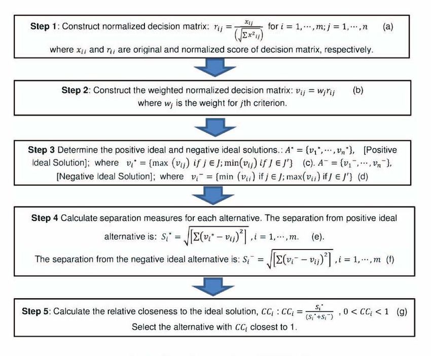
 19

Table 1 presents the variables in Equation 2 and Equation 3 with a description.

 Table 1: List of variables and their description

 Index Explanation Measurement
 One product Unit
 Customer Person

 k Purchase Order
 The sub-set of products carried Unit
 in the current inventory this season
 Budget – Restricted equity Euro
 The region, defined as country Discrete values 1 - 4
 The probability of a customer j Percent
 to select the product i in the product
 g j (i, M) sub-set M
 Expected Return Euro
 The quantity for the product i at Unit
 the beginning of the year
 The quantity of product i Unit
 The predicted demand for Unit
 product i on the website
 Euro
 Price for the product i
 Cost for the leftover inventory at Euro
 the end of the year
 Budget for the warehouse
 Seasonal growth Percent

 Figure 5: Localization model, input, and output

The third and last module is the localization mode and is to find the optimal location of the
warehouse (see Figure 5). This model is based on the TOPSIS model and the demand model.
As previously mentioned TOPSIS is an MCDM approach that can be used in any kind of area

 20

that includes decision-making of multiple criteria. Hence, TOPSIS is a comparison method. It
has been used in previous studies to decide where to locate the most optimal warehouse location
based on logistical factors. For the TOPSIS model, we will choose three criteria to compare
regions: 1-the level of competition, 2-customer population, and 3- best distance. The first
criteria, the LoC (level of competition) is the degree of how competitive regions are to each
other and can be explained by the number and relative size of buyers and sellers. This is
presented with a ranked list where 5 is high competition and 1 is low competition. The second
criterion, the CP (customer population) is defined as the number of customers clustered in one
region. The third criterion, the BD (best distance) is calculated through the distance from one
region to another. The best distance is the shortest path from one region to all other regions.
This is also presented with a ranked list where 5 is the shortest distance and 1 is the longest
distance. All these variables are equally important and therefore weighed equally. In Table 2
you can see the input for the TOPSIS model. The calculation of the TOPSIS model is presented
in the Appendix (See Table 1212, Table 1313, and Table 1414).

 Table 2: TOPSIS input model

 Weight (100 %) 0,333 (33,3 %) 0,333 (33,3 %) 0,333 (33,3 %)

 CP (nr of customers) LoC (rank) BD (rank)

 Netherlands 8790 5 3

 Germany 8102 4 5

 Poland 1131 4 1

 Austria 773 5 2

The demand model is not only used to gain the future demand of the products but also used to
further help find the optimal location of the warehouse. From the demand model, we gain
knowledge about the highest demand in different countries, defined as regions. The demand for
the products in the regions is thus further calculated through STATA through an MNL-
regression. It is composed of Equation 4

 Equation 4: STATA MNL demand model

 = 1 1 + 
 ln = ln 1 1 = 1 1
 ℎ 1 = ℎ , = 

 21

 1 = ℎ (log )
 1 = 
The region variable (Y) will be a categorized variable of (1 - 4) of the identified countries
regressed by the orders (X). The dependant variable (X1) is binary defined as 1 or zero and is
calculated through the first module (the demand module) of choosing a product to the
assortment or not. If the demand is higher than 50 % for a product then it will be set to 1,
otherwise, it will be set to zero. The output from the MNL regression will return a log-odds
value. By exponentiating the log odds, we will receive the odds of a product being bought in a
region/country.

Assumptions and delimitations have been done in all three steps of the optimization method.
For the demand model (first module) see the following:
 • All regions are offered the same set of products because the selling is made online,
 regardless of seasonal products. In other words, all products are available to
 purchase.
 • The range of products is equal in all regions.
 • There is no seasonal variation.
 • The total set of products will always be in stock.
 • Focus on the makeup category.
 • Top 70 products of each subcategory are selected for the demand model.
 • Each customer is associated with a single country since customers usually make
 purchases from the same country.
 • The utility for the demand model will be calculated through a ranked list of the
 popularity of a product.
For the optimization model (second module), see the following:
 • The offered set on the website is constant for every region since it is an e-tailer
 business.
 • Only budget, inventory, and demand constraints will be introduced.
For the TOPSIS model in the localization model (third module), see the following:
 • For factors that have been chosen: 1- customer population, 2- level of competition,
 3- best distance, 4- growth.
 • Variables equally distributed (same weight).

 22

4 RESULTS AND ANALYSIS: OPTIMIZING DEMAND,
 PRODUCTS, AND LOCATION
In this section, we will present the result from the optimization approach, which is divided into
three subsections, 1-demand model, 2-optimization model, and 3-localization model. An
analysis of each subsection will be made along with the results.

4.1 The products that are in high demand - The demand model
The result from the demand model using the MNL-regression gave us the products that are in
high demand and should be selected to the assortment. The following result was five products
from the Foundation category, zero products in the Primer category, seven products in the
Brows category, nine products in the Mascara category, six products in the Lipstick category,
five products in the Lipliner category, three products in the Blending Sponge category and only
one product in the Foundation Brush category. In total, there were 36 different products from
the Makeup category that were selected (See Table 10 in Appendix).

4.1.1 Interpretation of the demand model regarding the results
Given our constraints, there were only 36 products within the subset that were in high demand
and therefore selected to the assortment. However, since we only used less than 5 % (8 out of
300 categories) of the firm's total offered set of cosmetic products on the website, we expect
the outcome of the demand to be 95 % more for the whole offered set on their website.
 The products are characterized as non-seasonal products meaning that the sample data that
we use can be annual without it interfering with the statistical outcome. However, even though
the products are non-seasonal, they can be more popular during some seasons and less popular
during other seasons depending on the trend. This makes it important to consider data over a
longer period, for example, a year, to capture changes in the demand.
 When computing the probability of choosing product i from the sub-set M we had to scale
the output. Since we use a set of 70 different products in the demand calculation for each
subcategory, we used the relationship between these two to compute the scale factor (70/3).
The literature also states that the products above a 50 % probability of being chosen should be
selected to the assortment, making us scale down the lower limit of the probability to 0,022 %
(0,5/23). The reason for doing this is that the MNL model is a choice model, useful when
estimating demand for a group of products. Since we want to identify the demand for a single
product on a large scale set it will not be possible to use it as it is. This is because the MNL-

 23

model is a ratio of exponential functions, thus the probability will decrease significantly with
increased production. Based on this, the result will not be adaptable for a firm with large,
differentiated products. To adjust for this problem, we have scaled the output of the probability.
To scale the probability, we estimated that it should be 23 times larger than the original output.
The reason for this number (23) is that we assumed that for the MNL model to work properly,
it is appropriate to have some comparison groups, where three is a good size. This has been
examined many times in previous studies, for example, Crowson (2020), Grisolia & Willis
(2011), and Guadagni & Little (1983) which all have used three comparison groups in their
work.
 An interesting remark in our result is that most of the products (20/36 products) that are in
high demand belong to the firms that are in the top 10 firms in the cosmetics industry. MAC
and Clinique are brands of some of the products that were in high demand. These two brands
are subsidiaries of Estée Lauder. Rimmel is another brand that was also high in demand which
is owned by Coty Inc. Finally, Max Factor was also identified as one of the brands belonging
to the products in high demand. This brand is a subsidiary of Protector and Gamble (See Table
10 in Appendix).

4.2 The products that maximize profit - The optimization model
The output from the demand model was used as input for the optimizer (See Figure 7). Meaning
the products in high demand were entered through the optimization model to gain knowledge
about the products that maximize the profit of the firm. The result of the optimizer shows us
that 10 products maximize the profit of the firm within the selected subset and the profit of
these given the constraints was 65 223 Euro (See Table 3). The result that was given from the
optimizer returns the profit maximizing quantity of each selected product. This is done through
the optimization program Gurobi (See What is Gurobi Optimization in Appendix).
 Table 3: Data of the result from the optimization model

 Product number Category Product brand Product name Quantity Value
 X1 Foundation Rimmel Stay Matte 300 283
 Sand 30ml
 X6 Brows MAC Eye Brows Styler 86
 Spiked
 X7 Brows MAC Eye Brows Styler 159
 Stylized
 X22 Lipstick MAC FY21 BUY 3 GET 3 300

 24

X23 Lipstick Rimmel Provocalips Liquid 209
 Lipstick 730 Make
 You
 X24 Lipstick Essence glimmer GLOW 164
 lipstick
 X25 Lipstick Clinique F20 GFT 4CF 133
 SPRDF MST HV
 X28 Lipliner Essence STAY 8h 77
 WATERPROOF
 LIPLINER 01
 X33 Blending LYKO Powder Puff 58
 sponge
 X36 Foundation Real techniques Makeup Must 257
 Haves
 Brush

 Profit
 # Objective 65 223
 value

The products that maximize the profit are the following: x1 with 283 units in quantity, x6 with
86 units in quantity and x7 with 159 units in quantity, x22 with 300 units, x23 with 209 units x24
with 164 units, and x25 with 133 units in quantity, x28 with 77 units in quantity, x33 with 58 units
in quantity and x36 with 257 units in quantity. The total profit from these products was 65 223
Euro. The variables with their corresponding product name, brand, and category are shown in
Table 3 as well.

4.2.1 Understanding the optimization model and what products that maximize
 the profit given the constraints
For the optimization decision, products with positive expected value were considered in the
execution of the model since they are the products that can maximize profit. The higher the
probability of product i being chosen from the subset, the higher the demand. If the demand is
higher than last year’s sales for product i, the difference in cost between the quantity for product
i and the actual demand will be set to zero. Meaning that we will not have negative numbers in
the optimization and by achieving this, product i receives a higher value, which in turn increases
the profit. The goal will thus be to have zero leftover inventory at the end of the year. According

 25

to Farias et al., (2017) the key issue of assortment planning is to balance the loss of low-revenue
products with the gain of high-revenue products, as we can see from our demand model the
products being selected to maximize the profit are the ones with the highest revenue (See Table
15 in Appendix). Even Salmon (1993) states that many retailers use the strategy which seeks to
maximize the profit of product variety by eliminating low-selling products. Since the cost of a
product has a big impact on the model it is an important factor to consider. It is thus essential
to try to lower the purchase price of a product and have a higher mark-up price to get a better
marginal profit (See Table 15 in Appendix). Another parameter that impacts the result is the
growth of the market, the higher the growth the higher the demand for the product. We have
estimated the growth of the different markets to be equal across the countries/regions, making
α constant because the level of competition is high in all regions. Following Farias et al., (2017),
we decided to apply a seasonal growth factor α to the previous season’s sales since it provides
a rational prediction for future demand based on the market growth in the region. According to
our results, we discovered that a probability higher than 70 % of a customer choosing a product
from the subset, returns a positive outcome of the expected value for the product (See Table 10
and Table 15 in Appendix).
 In the optimization model, we scaled down the budget and sales constraint as well to fit the
model and data. The estimates were based on the firm's requirements of having 30 % of the
current production in the new warehouse. After receiving the demand for the next year, we only
used 30 % out of the restricted equity as the constraint for the budget.
 The optimization in Gurobi maximizes the first variable in the list. If it is optimized, it will
set the next variable to zero. Therefore, it is crucial to list the variables in the right prioritized
order. This also means that the optimizer does not make an even distribution between the
variables/products (Gurobi, 2022).
 By solving the demand problem, we can get knowledge about the products having the
highest demand and simultaneously offer the highest profit.

4.3 The optimal geographical solution for the warehouse
 location
When executing the MNL regression (See Equation 4) with different base outcomes for the
regions ((1) Germany, (2) Poland, (3) Netherlands, (4) Austria) we got the following results:

 26