On the suitability of second-order accurate finite-volume solvers for the simulation of atmospheric boundary layer flow
←
→
Page content transcription
If your browser does not render page correctly, please read the page content below
Geosci. Model Dev., 14, 1409–1426, 2021
https://doi.org/10.5194/gmd-14-1409-2021
© Author(s) 2021. This work is distributed under
the Creative Commons Attribution 4.0 License.

On the suitability of second-order accurate finite-volume solvers for
the simulation of atmospheric boundary layer flow
Beatrice Giacomini and Marco G. Giometto
Department of Civil Engineering and Engineering Mechanics, Columbia University in the City of New York,
500 W 120th St, New York, NY 10027, USA

Correspondence: Marco G. Giometto (mg3929@columbia.edu)

Received: 31 March 2020 – Discussion started: 13 May 2020
Revised: 14 December 2020 – Accepted: 27 December 2020 – Published: 15 March 2021

Abstract. The present work analyzes the quality and re-               an enhanced sensitivity of the solution to variations in grid
liability of an important class of general-purpose, second-           resolution, thus calling for future research aimed at reducing
order accurate finite-volume (FV) solvers for the large-eddy          the impact of modeling and discretization errors.
simulation of a neutrally stratified atmospheric boundary
layer (ABL) flow. The analysis is carried out within the
OpenFOAM® framework, which is based on a colocated
grid arrangement. A series of open-channel flow simulations           1   Introduction
are carried out using a static Smagorinsky model for sub-
grid scale momentum fluxes in combination with an alge-               An accurate prediction of atmospheric boundary layer (ABL)
braic equilibrium wall-layer model. The sensitivity of the            flows is of paramount importance across a wide range of
solution to variations in numerical parameters such as grid           fields and applications, including weather forecasting, com-
resolution (up to 1603 control volumes), numerical solvers,           plex terrain meteorology, agriculture, air quality modeling,
and interpolation schemes for the discretization of nonlin-           and wind energy (Whiteman, 2000; Fernando, 2010; Calaf
ear terms is evaluated and results are contrasted against             et al., 2010; Oke et al., 2017; Shaw et al., 2019).
those from a well-established mixed pseudospectral–finite-               Since the early work of Deardorff (1970), the large-eddy
difference code. Considered flow statistics include mean              simulation (LES) technique has spurred considerable in-
streamwise velocity, resolved Reynolds stresses, velocity             sight on the fundamental dynamics of ABL flow over rough
skewness and kurtosis, velocity spectra, and two-point auto-          surfaces (Anderson and Meneveau, 2010; Salesky et al.,
correlations. A quadrant analysis along with the examination          2017; Momen et al., 2018), over and within plant and urban
of the conditionally averaged flow field are performed to in-         canopies (Yue et al., 2007b; Bailey and Stoll, 2013; Pan et al.,
vestigate the mechanisms responsible for momentum trans-              2014; Tseng et al., 2006; Bou-Zeid et al., 2009; Giometto
fer in the flow. It is found that at the selected grid resolutions,   et al., 2017; Li and Bou-Zeid, 2019), and for wind energy
the considered class of FV-based solvers yields a poorly cor-         applications (Calaf et al., 2010; Abkar and Porté-Agel, 2013;
related flow field and is not able to accurately capture the          Stevens and Meneveau, 2017), amongst others.
dominant mechanisms responsible for momentum transport                   The majority of the past work has relied on fully or
in the ABL. Specifically, the predicted flow field lacks the          partially dealiased mixed pseudospectral–finite-difference
well-known sweep and ejection pairs organized side by side            (PSFD) solvers – the go-to approach for LES studies since
along the cross-stream direction, which are representative of         the works of Moin et al. (1978) and Moeng (1984). Such
a streamwise roll mode. This is especially true when using            solvers are known to yield accurate flow fields up to the
linear interpolation schemes for the discretization of nonlin-        LES cutoff frequency and to produce good results when used
ear terms. This shortcoming leads to a misprediction of flow          in conjunction with dynamic subgrid scale (SGS) models
statistics that are relevant for ABL flow applications and to         (Germano et al., 1991; Lilly, 1992). However, single domain
                                                                      PSFD-based solvers are limited to regular domains, are not

Published by Copernicus Publications on behalf of the European Geosciences Union.
1410                        B. Giacomini and M. G. Giometto: On the suitability of general-purpose finite-volume solvers

suitable for the simulation of nonperiodic flows, have sharp        liers, 2006; Jasak et al., 2007). A suite of simulations is car-
variations in the flow field such as shocks or fluid–solid in-      ried out varying physical and numerical parameters, includ-
terfaces in boundary layer flows, and are typically difficult to    ing grid resolution (up to 1603 control volumes), the numer-
parallelize owing to the global support of their spatial rep-       ical solver, and interpolation schemes for the discretization
resentation (see, e.g., Margairaz et al., 2018). With the in-       of the nonlinear term. Predictions from the FV solvers are
creasing need to account for complex geometries and multi-          contrasted against the results from the Albertson and Par-
physics, several efforts have been devoted to the mitigation        lange (1999) PSFD code in terms of flow statistics, including
of the aforementioned limitations (Fang et al., 2011; Li et al.,    mean streamwise velocity, resolved Reynolds stresses, two-
2016; Chester et al., 2007). However, the solutions are often       point velocity autocorrelations, and mechanisms supporting
ad hoc or validated only for specific applications, thus intro-     momentum transport. The end goal is to provide a more nu-
ducing a degree of uncertainty in model results that is hard        anced understanding of the capabilities of general-purpose,
to quantify and generalize.                                         second-order, FV-based solvers in predicting ABL flow.
   There is hence a growing interest from the ABL commu-               The work is organized as follows. Section 2 summarizes
nity in LES solvers based on compact spatial schemes via            the setup of the problem, the simulation database, and the
structured or unstructured meshes (Orlandi, 2000; Ferziger          postprocessing procedure. Results are shown in Sect. 3 and
and Peric, 2002). The parallelized large-eddy simulation            conclusions are drawn in Sect. 4. A further discussion on the
model (Raasch and Schröter, 2001; Maronga et al., 2015) and         sensitivity of the solution to model constants, interpolation
the weather research and forecasting model (Skamarock and           schemes, and numerical solvers is provided in the Appendix.
Klemp, 2008; Powers et al., 2017) are prominent examples
of said efforts. Both the approaches are based on a high-
order finite-difference discretization, with nonlinear terms        2     Methodology
approximated by using high-order upwind biased differenc-
                                                                    2.1    Governing equations and numerical schemes
ing schemes. The latter are suitable for LES in complex ge-
ometries with arbitrary grid stretching factors and outflow         We use index notation in a Cartesian reference system. The
boundary conditions (Beaudan and Moin, 1994; Mittal and             spatially filtered Navier–Stokes equations are considered,
Moin, 1997) but are dissipative and do not strictly conserve
energy. On the other hand, if central schemes are used instead                                               SGS,dev
                                                                    ∂ui      ∂ui    1 ∂ p̃ ∂τij ∂τij                       1 ∂P
for the evaluation of nonlinear terms, no numerical dissipa-            + uj     =−       −     −                      −         , (1)
tion is introduced, but truncation errors can have an over-         ∂t       ∂xj    ρ ∂xi   ∂xj    ∂xj                     ρ ∂xi
whelming impact on the computed flow field (Ghosal, 1996;           ∂ui
                                                                        =0 ,                                                       (2)
Kravchenko and Moin, 1997). These limitations typically re-         ∂xi
sult in a strong sensitivity of the solution to properties of the
spatial discretization and numerical scheme (Meyers et al.,         where ui = (u, v, w) is the spatially filtered velocity field
2006, 2007; Meyers and Sagaut, 2007; Vuorinen et al., 2014;         along the streamwise (x), cross-stream (y), and vertical (z)
Rezaeiravesh and Liefvendahl, 2018; Breuer, 1998; Montec-           coordinate directions, respectively, t is the time, ρ is the
chia et al., 2019). Further, truncation errors corrupt the high     constant fluid density (Boussinesq approximation), p̃ ≡ p +
                                                                    1 SGS
wavenumber range of the solution, restricting the ability to        3 τkk is a modified pressure term, τij is the filtered viscous
adopt dynamic LES closure models that make use of infor-            stress tensor, and τijSGS,dev is the deviatoric part of the SGS
mation from the smallest resolved scales of motion to evalu-        stress tensor. In addition, the term − ρ1 ∂x
                                                                                                              ∂P
                                                                                                                 i
                                                                                                                   is an imposed con-
ate the SGS diffusion (Germano et al., 1991). Notwithstand-         stant pressure gradient driving the flow. The spatially filtered
ing these limitations, central schemes have been heavily em-        viscous tensor is τij = −2νSij , where ν = const is the kine-
ployed in the past in both the geophysical and engineering          matic viscosity of the Newtonian fluid and Sij is the resolved
flow communities and are the de facto standard in the wind          (in the LES sense) rate of strain tensor. For the SGS stress
engineering community, where most of the numerical sim-             tensor, the static Smagorinsky model is used,
ulations are carried out using second-order accurate finite-
volume (FV)-based solvers (Stovall et al., 2010; Churchfield        τijSGS,dev = −2ν SGS Sij = −2(CS 1)2 |S|Sij ,                  (3)
et al., 2010; Balogh et al., 2012; Churchfield et al., 2013; Shi
and Yeo, 2016, 2017; García-Sánchez et al., 2017; García-           where ν SGS is the SGS eddy viscosity, CS is the Smagorin-
Sánchez and Gorlé, 2018).                                           sky coefficient (Smagorinsky, 1963), 1 = (1x1y1z)1/3 is
   Motivated by the aforementioned needs, the present study         a local length scale based on the volume of p the computa-
aims at characterizing the quality and reliability of an impor-     tional cell (Scotti et al., 1993), and |S| = 2Sij Sij quan-
tant class of second-order accurate FV solvers for the LES          tifies the magnitude of the rate of strain. In the present
of neutrally stratified ABL flows. The analysis is conducted        work, CS = 0.1, unless otherwise specified. Note that dy-
in the open-channel flow setup (no Coriolis acceleration) via       namic Smagorinsky models are preferred to the static one
the OpenFOAM® framework (Weller et al., 1998; De Vil-               for the LES of ABL flows (Germano et al., 1991; Lilly,

Geosci. Model Dev., 14, 1409–1426, 2021                                              https://doi.org/10.5194/gmd-14-1409-2021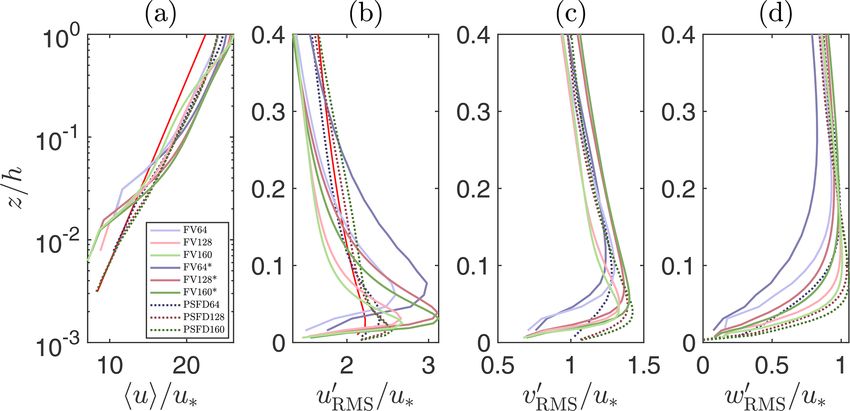
B. Giacomini and M. G. Giometto: On the suitability of general-purpose finite-volume solvers 1411
p
1992; Meneveau and Lund, 1997; Porté-Agel, 2004; Bou- the definition of friction velocity u∗ = τw2 , where τw is the
Zeid et al., 2005). Dynamic models evaluate SGS stresses magnitude of the kinematic wall shear stress vector, along
via first-principles-based constraints, feature improved dissi- with Eq. (5), and rearranging, the total eddy viscosity at the
pation properties when compared to the static Smagorinsky wall can be written as
model (especially in the vicinity of solid boundaries), and 2
are free of explicit modeling parameters. The choice made in
κ|ũ|c 1z
the present study is motivated by problematics encountered νt,f = (7)
1z |ũ|c − ν ,
when using the available dynamic Lagrangian model in pre- ln
liminary tests. However, while SGS dissipation plays a cru- z0
cial role in PSFD solvers, truncation errors may overshadow which is the formulation implemented herein. Note that
SGS stress contributions in the second-order FV-based ones ν + νt ≈ νt in the boundary layer flows in the fully rough
(Kravchenko and Moin, 1997). The static Smagorinsky SGS aerodynamic regime, so ν could be neglected without loss
model used herein might hence perform similarly to dynamic of accuracy.
SGS models for the considered flow setup. This conjecture is In the present work, the computational grid is colocated,
supported by the results of Majander and Siikonen (2002). being the only colocated grid arrangement available within
The large scale separation between near-surface and outer- the OpenFOAM® framework. Note that although advanta-
layer energy-containing ABL motions poses stringent res- geous in complex domains when compared to staggered grids
olution requirements to numerical modelers, if all the en- (Ferziger and Peric, 2002), the colocated arrangement is
ergy containing motions have to be resolved. To reduce the known to cause difficulties with pressure–velocity coupling,
computational cost of such simulations, the near-surface re- hence requiring specific procedures to avoid oscillations in
gion is typically bypassed and a phenomenological wall- the solution. OpenFOAM® offers the standard Rhie–Chow
layer model is leveraged instead to account for the impact correction (Rhie and Chow, 1983), which is known to neg-
of near-wall (inner-layer) dynamics on the outer-layer flow atively affect the energy-conservation properties of central
(Piomelli, 2008; Bose and Park, 2018). This approach is re- schemes (Ferziger and Peric, 2002). In addition, when ap-
ferred to as wall-modeled large-eddy simulation (WMLES) proximating the integrals over the surfaces bounding each
and is used herein. An algebraic wall-layer model for sur- control volume (as a consequence of the Gauss divergence
faces in a fully rough aerodynamic regime was implemented theorem), the unknowns are evaluated at face centers and
based on the logarithmic equilibrium assumption, i.e., are assumed to be constant at each face, yielding an over-
u∗
z all second-order spatial accuracy (Churchfield et al., 2010).
|ũ| = ln , (4) Since the divergence form of the convective term is used in
κ z0
combination with a low-order scheme over a nonstaggered
√ grid, the solution is inherently unstable (Kravchenko and
where |ũ| ≡ u2 + v 2 is the norm of the velocity at a certain
distance from the ground level, u∗ is the friction velocity (see Moin, 1997). The present work makes use of the linear and
Sect. 2.2 for details), κ is the von Kármán constant, z is the QUICK interpolation schemes (Ferziger and Peric, 2002) to
distance from the ground level, and z0 is the so-called aero- evaluate the unknowns at face centers (more details are pro-
dynamic roughness length, a length scale used to quantify vided in Sect. 2.2). The numerical solver is based on the
the drag of the underlying surface. In this work, the values PISO algorithm (Issa, 1985) for the pressure–velocity calcu-
κ = 0.41 and z0 = 0.1 m are set. The kinematic wall shear lation and on an implicit Adams–Moulton scheme for time
stress is assumed to be proportional to the local velocity gra- integration (Ferziger and Peric, 2002). In Appendix A2, the
dient (Boussinesq hypothesis), performances of an alternative solver with a Runge–Kutta
time-advancement scheme and a projection method for the
∂ui pressure–velocity coupling (Vuorinen et al., 2014) are ana-
τiz,w = (ν + νt ) |w , i = x, y , (5)
∂z lyzed.
where νt is the total eddy viscosity. Employing the no-slip 2.2 Problem setup
condition for the velocity field, the standard FV approxima-
tion of the shear stress at the wall gives (Mukha et al., 2019) A series of WMLES of ABL flow (open-channel flow setup)
ui,c is performed. Tests are carried out in the domain [0, Lx ] ×
τiz,w = (ν + νt )f , i = x, y , (6) [0, Ly ] × [0, Lz ] with Lx = 2π h, Ly = 43 π h, Lz = h, where
1z
h = 1000 m denotes the width of the open channel. Symme-
where the subscript f is used to denote the evaluation at the try is imposed at the top of the computational domain, no-slip
center of the wall face, the subscript c denotes the evaluation applies at the lower surface, and periodic boundary condi-
at the center of the wall-adjacent cell, and 1z is the distance tions are enforced along each side. A kinematic pressure gra-
from the wall. From the logarithmic law (Eq. 4) evaluated at dient term − ρ1 ∂P 2
∂x = 1 m/s drives the flow along the x coor-
the first cell center, one can write u∗ = κ|ũ|c / ln( 1z
z0 ). Using dinate direction, yielding u∗ = 1 m/s. The kinematic viscos-
https://doi.org/10.5194/gmd-14-1409-2021 Geosci. Model Dev., 14, 1409–1426, 2021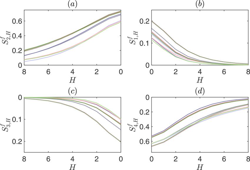
1412                        B. Giacomini and M. G. Giometto: On the suitability of general-purpose finite-volume solvers

ity is set to a nominal value of 10−7 m2 /s, which results in      of the flow (Kawai and Larsson, 2012). The LLM is partic-
an essentially inviscid flow.                                      ularly pronounced for the cases using the QUICK interpola-
   The computational mesh is Cartesian, with a uniform sten-       tion scheme. This behavior could have been anticipated, as
cil along each direction. Three simulations are run over 643 ,     the wall shear stress is evaluated using the instantaneous hor-
1283 , and 1603 control volumes, with the linear interpolation     izontal velocity at the first cell center off the wall. A num-
scheme for the evaluation of the unknowns at the face cen-         ber of procedures has been proposed to alleviate the LLM,
ters (simulations FV64, FV128, and FV160, respectively).           including modifying the SGS stress model in the near-wall
Three additional simulations are run, at the same grid reso-       region (Sullivan et al., 1994; Porté-Agel et al., 2000; Chow
lutions, with the linear scheme for the approximation of ev-       et al., 2005; Wu and Meyers, 2013), shifting the matching
ery term except for the nonlinear one, for which the QUICK         location further away from the wall (Kawai and Larsson,
scheme is used instead (simulations FV64*, FV128*, and             2012), and carrying out a local horizontal/temporal filtering
FV160*). The cases span different grid resolutions at the          operation (Bou-Zeid et al., 2005; Xiang et al., 2017). In pre-
same aspect ratio 1x/1z = 2π . Note that the chosen grid           liminary runs, the approach of Kawai and Larsson (2012)
resolutions are in line with those typically used in studies       was implemented in an attempt to alleviate the LLM. How-
of ABL flow with the pseudospectral approach (see, e.g.,           ever, no apparent improvement was observed and the solu-
Salesky et al., 2017). All the calculations satisfy the Courant–   tion became very sensitive to grid resolution and matching
Friedrichs–Lewy (CFL) condition C.0.1, where C is the              location. This finding suggests that alternative procedures
Courant number. Runs are initialized from a fully developed        might need to be devised to overcome the LLM in ABL flow
open-channel flow simulation in statistically steady state (dy-    simulations when using the considered class of FV solvers.
namic equilibrium), and time integration is carried out for        Note that profiles from the PSFD solver also feature a pos-
100 eddy turnover times, where the eddy turnover time is           itive LLM in spite of a spatial, low-pass filtering operation
defined as h/u∗ . Flow statistics are the result of an averag-     that is carried out on the horizontal velocity field before eval-
ing procedure over the horizontal plane of statistical homo-       uating the surface shear stress (Bou-Zeid et al., 2005).
geneity of turbulence (xy) and in time over the last 60 eddy          The vertical structure of turbulence intensities is also
turnover times. The procedure yields well-converged statis-        shown in Fig. 1, where (·)0RMS denotes the root mean square
tics throughout the considered cases. In the following, the        (RMS) of the fluctuations. Profiles from the FV-based solver
horizontal and temporal averaging operation is denoted by          start off relatively slow at the wall when compared to those
h·i. The results from the present study are contrasted against     from the PSFD-based solver and to the reference profile from
the corresponding ones from the Albertson and Parlange             Hultmark et al. (2013). This behavior is due to a combination
(1999) mixed PSFD code (simulations PSFD64, PSFD128,               of SGS and discretization errors, which damp the energy of
and PSFD160). The code is based on an explicit second-order        high-wavenumber modes and whose accurate quantification
accurate Adams–Bashforth scheme for time integration and           remains an open challenge in LES (see, e.g., Meyers et al.,
on a fractional-step method for solving the system of equa-        2006; Meyers and Sagaut, 2007; Meyers et al., 2007). Fur-
tions. Simulations from the PSFD solver are carried out us-        ther aloft, u0RMS (wRMS
                                                                                        0    ) features relatively stronger (weaker)
ing a static Smagorinsky SGS model with CS = 0.1, a rough          peak values when compared to the corresponding PSFD pro-
wall-layer model with z0 = 0.1 m, and C.0.1. A summary             file, the overprediction (underprediction) being more appar-
of the runs is given in Table 1 along with the acronyms used       ent in the simulations with the QUICK scheme. The over-
in this study.                                                     shoot in the peak of u0RMS is a well-known problem of FV-
                                                                   based WMLES (Bae et al., 2018). Lack of energy redistri-
                                                                   bution via pressure fluctuation from shear generated u0RMS
                                                                         0
                                                                   to vRMS           0
                                                                              and wRMS    is the root cause of said behavior, and
3     Results
                                                                   possible mitigation strategies include allowing for wall tran-
This section is devoted to the analysis of velocity central        spiration (Bose and Moin, 2014). Grid refinement shifts the
moments (Sect. 3.1), spectra and spatial autocorrelations          velocity RMS peaks closer to the surface and increases the
(Sect. 3.2), and momentum transfer mechanisms (Sect. 3.3).         magnitude of the velocity RMS therein, but leads to no im-
                                                                   provement in the max(u0RMS ) and only marginally improves
                                                                   the estimation of the max(wRMS  0   ). A quantitative measure of
3.1    Mean velocity, Reynolds stresses, and higher-order
                                                                                           0
                                                                   the relative error on uRMS with respect to the reference profile
       statistics
                                                                   u0RMS,ref from Hultmark et al. (2013) in the z0 / h ≤ z/ h ≤
Figure 1 shows first- and second-order statistics for all the      0.4 interval is shown in Table 2. The FV-based solver per-
considered cases. The mean streamwise velocity is shown            forms worse than the PSFD-based one and the convergence is
in Fig. 1a in a comparison with the phenomenological               not monotonic. Note that nonmonotonic convergence is rel-
logarithmic-layer profile. The velocity at the first two cell      atively common in LES at relatively coarse resolutions and
centers off the wall is consistently underpredicted, whereas       is due to the interaction between discretization and model-
a positive log-layer mismatch (LLM) is observed in the bulk

Geosci. Model Dev., 14, 1409–1426, 2021                                             https://doi.org/10.5194/gmd-14-1409-2021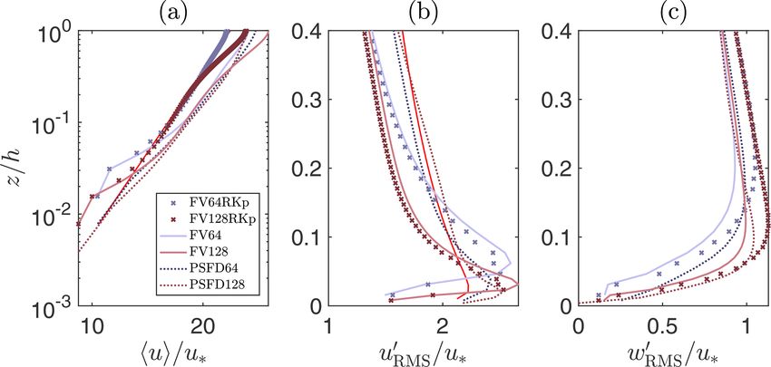
B. Giacomini and M. G. Giometto: On the suitability of general-purpose finite-volume solvers                                                1413

Table 1. Tabulated list of cases.

  Simulation           FV64     FV128      FV160      FV64*             FV128*            FV160*           PSFD64       PSFD128      PSFD160
  Nx × Ny × Nz         643      1283       1603       643               1283              1603             643          1283         1603
  Numerical solver     FV       FV         FV         FV + QUICK        FV + QUICK        FV + QUICK       PSFD         PSFD         PSFD

Figure 1. Vertical structure of mean streamwise velocity hui/u∗ (a), streamwise velocity RMS u0RMS /u∗ (b), cross-stream velocity RMS
 0
vRMS                                        0
      /u∗ (c), and vertical velocity RMS wRMS    /u∗ (d). The red line in (a) denotes the reference logarithmic profile and the red line in (b) is
a reference profile from Hultmark et al. (2013).

ing errors, whose impact on the solution cannot be a priori                against the phenomenological production range and inertial
quantified (Meyers et al., 2007).                                          subrange power-law profiles (k −1 and k −5/3 , respectively).
   Skewness and kurtosis of the streamwise velocity (Suu and               Predictions from the PSFD-based solver feature a relatively
Kuu , respectively) are shown in Fig. 2. The profiles of Suu               good agreement with the phenomenological power-law pro-
obtained with the FV-based solver and the QUICK scheme                     file, especially at high grid resolution. For example, the cases
as well as those obtained with the PSFD-based solver are                   PSFD128 and PSFD160 exhibit a slope of −1.2 in the pro-
in good agreement with experimental results from Monty                     duction range (here defined as kx z < 1). Profiles from the
et al. (2009), here taken as a reference. On the contrary, the             FV-based solver, on the contrary, exhibit strong sensitivity to
FV-based solver overpredicts Suu when the linear interpola-                grid resolution and are unable to capture the expected power-
tion scheme is used, with the skewness remaining positive                  law behavior. In the production range, velocity spectra from
throughout the whole extent of the surface layer. Note that                the FV solver start off relatively shallow at small wavenum-
a positive skewness of streamwise velocity represents a flow               ber, especially when using the linear scheme. A narrow band
field where negative fluctuations are more likely to happen                can be identified where Euu ∼ (kx z)−1 , followed by a rapid
than the corresponding positive ones. The kurtosis obtained                decay in energy density – the decay being particularly pro-
with the FV-based solver is consistently overpredicted, rep-               nounced when using the QUICK interpolation scheme be-
resenting a flow field populated by a greater number of ex-                cause of the associated numerical dissipation. Overall, the
treme events. Again, profiles from all cases feature a non-                energy density in the production range and in the inertial
monotonic convergence to the reference ones, as shown in                   subrange is not well captured by the FV-based solver and
Table 3, where the relative error on skewness and kurtosis                 grid refinement does not help circumvent this limitation, at
with respect to the measurements from Monty et al. (2009) is               least at the considered resolutions. The authors note that this
reported in the interval z0 / h ≤ z/ h ≤ 0.4.                              fact might limit the use of dynamic procedures based on the
                                                                           Germano et al. (1991) identity. A further characterization of
3.2   Spectra and autocorrelations                                         the energy distribution in the wavenumber space is given in
                                                                           Fig. 3b, where premultiplied velocity spectra kx Euu u−2  ∗ are
                                                                           shown. The usual reason for considering these quantities is
One-dimensional spectra of streamwise velocity fluctuations
                                                                           to create a plot in semi-log scale where equal areas under
(Euu ) are shown in Fig. 3a. The profiles are contrasted

https://doi.org/10.5194/gmd-14-1409-2021                                                        Geosci. Model Dev., 14, 1409–1426, 2021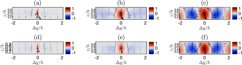
1414                          B. Giacomini and M. G. Giometto: On the suitability of general-purpose finite-volume solvers

Table 2. Relative error on the turbulence intensities ||u0RMS − u0RMS,ref ||L2 /||u0RMS,ref ||L2 w.r.t. the reference profile from Hultmark et al.
(2013) in the interval z0 / h ≤ z/ h ≤ 0.4.

        Simulation                  FV64     FV128      FV160     FV64*      FV128*      FV160*      PSFD64       PSFD128      PSFD160
        Relative error on u0RMS     0.23     0.17       0.17      0.28       0.20        0.20        0.10         0.05         0.07

Figure 2. Vertical structure of skewness of streamwise velocity (a) and kurtosis of streamwise velocity (b). Lines are defined in Fig. 1. The
red x-marks denote the measurements from Monty et al. (2009), digitalized by the authors.

the profiles correspond to equal energy. In addition, premul-              tal extent of the computational domain. The authors have in-
tiplied spectra provide information on the coherence of the                deed verified that a larger domain (twice as large along each
flow, in particular on the so-called large and very large scale            horizontal direction) enables one to capture LSMs with the
motions (LSMs and VLSMs, respectively). These structures                   PSFD solver at resolutions matching the one of the PSFD128
are responsible for carrying more than half of the kinetic                 case (not shown). A corresponding single run was carried out
energy and Reynolds shear stress and are a persistent fea-                 with the FV solver over the said larger domain and premulti-
ture of the surface and outer layers of both aerodynamically               plied spectra were found to be in good agreement with those
smooth and rough walls (Kim and Adrian, 1999; Balakumar                    presented herein, supporting the conjecture that the proposed
and Adrian, 2007; Monty et al., 2007; Hutchins and Maru-                   domain size suffices to capture the range of variability of FV
sic, 2007; Fang and Porté-Agel, 2015). The current domain                  solvers for the problem under consideration.
is of modest dimensions and is able to accommodate only                       To gain better insight on the spatial coherence of the flow
LSMs (Lozano-Durán and Jiménez, 2014), which are iden-                     field, the contour lines of the two-dimensional autocorrela-
tified in premultiplied spectra by a local maximum at the                                                    2D in the xy plane are shown
                                                                           tion of the streamwise velocity Ruu
streamwise wavenumber kx / h ≈ 1. The location of the peaks                                 2D
                                                                           in Fig. 4. The Ruu = 0.1 contour is often used to identify the
from the FV-based solver with linear interpolation scheme                  boundaries of coherent structures populating the flow field.
shifts toward higher wavenumber with grid refinement, with                 The contours from the FV-based solver with linear scheme
a maximum at kx / h ≈ 4 for the FV160 case. This fact sig-                 (Figs. 4a, d) are representative of a poorly correlated flow
nals a flow field where the streamwise extent of energetic                 field with a streamwise extent of the Ruu 2D = 0.1 contour of

modes (a.k.a., coherent structures) reduces as the grid is re-             0.5h and 0.1h along the streamwise and cross-stream direc-
fined. On the contrary, the FV-based solver in combination                 tions, respectively. On the contrary, the contours from the
with the QUICK scheme predicts the peak in premultiplied                   FV-based solver with the QUICK scheme (Fig. 4b, e) depict
energy density at the expected wavenumber, hence suggest-                  a flow field characterized by larger spatial autocorrelation,
ing that this approach is able to capture LSMs. The PSFD-                  in line with results from the PSFD-based solver. Note that
based solver features a peak at the expected wavenumber                    the flow statistics presented above should not be impacted
(kx = 1) only at the lowest resolution (PSFD64). Profiles                  by the fact that the current domain size prevents some of
from the higher-resolution cases feature high energy densi-                the contour lines (simulations FV64*, FV160*, PSFD64, and
ties at the lowest wavenumber, highlighting an artificial “pe-             PSFD160) from closing, as discussed in Lozano-Durán and
riodization” of energy-containing structures in the stream-                Jiménez (2014).
wise direction. This behavior is linked to the limited horizon-

Geosci. Model Dev., 14, 1409–1426, 2021                                                         https://doi.org/10.5194/gmd-14-1409-2021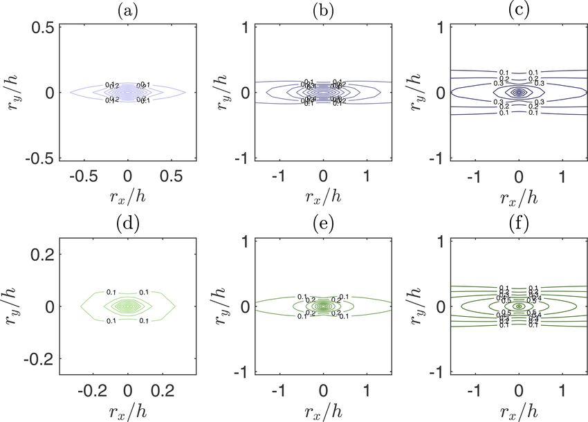
B. Giacomini and M. G. Giometto: On the suitability of general-purpose finite-volume solvers 1415
Table 3. Relative error on skewness ||Suu − Suu,meas ||L2 /||Suu,meas ||L2 and kurtosis ||Kuu − Kuu,meas ||L2 /||Kuu,meas ||L2 w.r.t. the mea-
surements from Monty et al. (2009) in the interval z0 / h ≤ z/ h ≤ 0.4.
Simulation FV64 FV128 FV160 FV64* FV128* FV160* PSFD64 PSFD128 PSFD160
Relative error on Suu 1.63 1.77 1.81 0.86 0.75 0.71 0.51 0.57 0.68
Relative error on Kuu 0.28 0.25 0.25 0.23 0.16 0.15 0.11 0.05 0.04
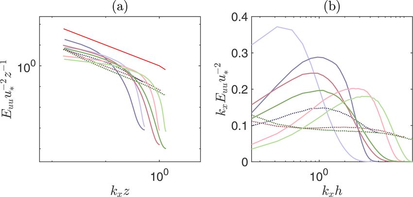
Figure 3. (a) Normalized one-dimensional spectra of streamwise velocity at z/ h ≈ 0.1. The solid red line depicts the (kx z)−1 production
range and (kx z)−5/3 inertial subrange scaling. All other lines as in Fig. 1. (b) Premultiplied one-dimensional spectra of streamwise velocity
at z/ h ≈ 0.1.
The one-dimensional spatial autocorrelation (Ruu ), shown correlation function, it is apparent that the FV-based solver
in Fig. 5 along the streamwise and cross-stream directions, underestimates the integral lengths when compared to the
further corroborates the above findings. From Fig. 5a it is PSFD cases and the reference DNS values, especially when
apparent that the extension of the selected domain does not the linear interpolation scheme is used.
enable the flow to become completely uncorrelated in the Instantaneous snapshots of streamwise velocity fluctua-
streamwise direction for the PSFD solver and for the FV tions over a horizontal plane support the above findings (see
solver using QUICK; Ruu remains finite in the available rx / h Fig. 6). Artificially periodized, streamwise-elongated bulges
range across resolutions. On the other hand, profiles from of uniform high and low momentum are indeed apparent in
the FV-based solver using the linear interpolation rapidly de- the snapshots from the PSFD-based solver (Fig. 6c, f). On the
cay towards zero. Along the cross-stream direction (Fig. 5b), contrary, the instantaneous streamwise velocity field from the
profiles from the PSFD-based solver feature the expected FV solver is populated by smaller regions of uniform mo-
negative lobes, highlighting the presence of high- and low- mentum, especially when using the linear scheme, and the
momentum streamwise-elongated streaks flanking each other size of energetic structures diminishes with increasing grid
in the said direction. This behavior is in line with findings resolution (see, e.g., Fig. 6a, d).
from previous studies on the coherence of wall-bounded tur-
bulence and with standard turbulence theory. Profiles from 3.3 Momentum transfer mechanisms
the FV-based solver exhibit a similar profile, albeit featur-
ing a more rapid decay and less prominent negative lobes, This section is devoted to the analysis of momentum transfer
especially for the high-resolution cases using the linear in- mechanisms in the ABL with a focus on quadrant analysis
terpolation scheme. A quantitative measure of the coherence (Lu and Willmarth, 1973) and on statistics of conditionally
of the flow field is provided in Table 4, where the integral averaged flow fields.
lengths 3rx ,u and 3ry ,u are reported for all the considered The quadrant hole analysis is a technique based on the de-
cases and compared against direct numerical simulations of composition of the velocity fluctuations into four quadrants:
a channel flow at Reτ = 2000 from Sillero et al. (2014). The the first and third quadrants, outward interactions (u0 > 0,
integral lengths in Table 4 are evaluated at z/ h ≈ 0.15 since w 0 > 0) and inward interactions (u0 < 0, w0 < 0), respec-
the data from Sillero et al. (2014) are available at this height. tively, are negative contributions to the momentum flux,
Although 3rx ,u might not be meaningful across the consid- whereas the second and fourth quadrants, a.k.a. ejections of
ered cases, owing to the lack of a zero crossing of the auto- low-speed fluid outward from the wall (u0 < 0, w0 > 0) and
https://doi.org/10.5194/gmd-14-1409-2021 Geosci. Model Dev., 14, 1409–1426, 2021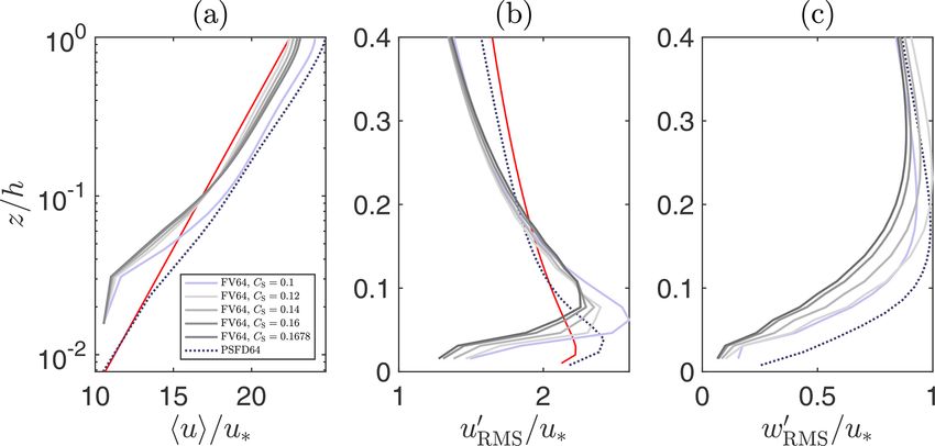
1416                         B. Giacomini and M. G. Giometto: On the suitability of general-purpose finite-volume solvers

Figure 4. Contours of two-dimensional spatial autocorrelation of streamwise velocity at height z/ h ≈ 0.1 from the simulations FV64 (a),
FV64* (b), PSFD64 (c), FV160 (d), FV160* (e), and PSFD160 (f). Contour levels from 0.1 to 0.9 with increments of 0.1.

Figure 5. One-dimensional spatial autocorrelation of streamwise velocity at height z/ h ≈ 0.1 along the streamwise direction (a) and along
the cross-stream direction (b). Lines as in Fig. 1.

sweeps of high-speed fluid toward the wall (u0 > 0, w0 < 0),           Reynolds shear stress from more extreme events. Clearly, the
represent positive contributions. A range of flow statistics can       FV-based solver with the linear scheme underpredicts ejec-
be defined based on this decomposition and used to provide             tions (Fig. 7a), outward interactions (Fig. 7b), and inward
insight on the mechanisms supporting momentum transfer in              interactions (Fig. 7c), and overpredicts sweeps at large hole
the ABL.                                                               size H (Fig. 7d). On the contrary, the FV solver with the
   Figure 7 features the quadrant-hole analysis, where the no-         QUICK scheme underpredicts all the profiles except for the
tation is the same as in Yue et al. (2007a), with H being the          ejections, which are captured fairly well instead (see Fig. 7a).
hole size, Si,H the resolved Reynolds shear stress contribu-           Note that ejections are violent events, concentrated over a
                                                f                      very thin region in the cross-stream direction of the ABL
tion to the ith quadrant at hole size H , and Si,H is the cor-
responding quadrant fraction. Stress fractions are presented           (Fang and Porté-Agel, 2015).
for values of the hole size H ranging from 0 to 8, where                  To gain insight on the vertical structure of momentum
larger hole sizes correspond to contributions to the resolved          transfer mechanisms, the exuberance ratio and the ratio of

Geosci. Model Dev., 14, 1409–1426, 2021                                                  https://doi.org/10.5194/gmd-14-1409-2021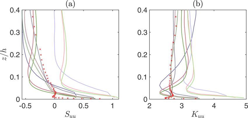
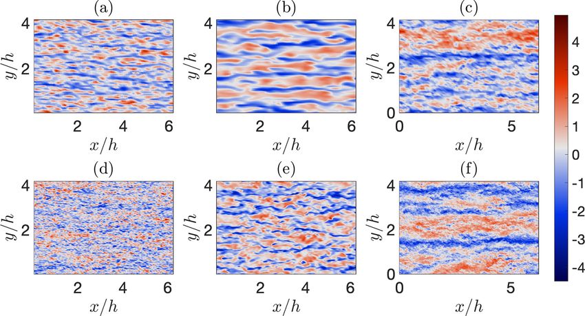
B. Giacomini and M. G. Giometto: On the suitability of general-purpose finite-volume solvers                                       1417

Table 4. Integral lengths at height z/ h ≈ 0.15.

  Simulation     FV64     FV128      FV160     FV64*   FV128*     FV160*     PSFD64      PSFD128     PSFD160      Sillero et al. (2014)
  3rx ,u / h     0.23     0.12       0.11      0.82    0.59       0.59       1.28        1.50        1.45         2.14
  3ry ,u / h     0.04     0.03       0.03      0.10    0.08       0.08       0.14        0.15        0.14         0.20

Figure 6. Instantaneous snapshots of normalized streamwise velocity fluctuations at z/ h ≈ 0.1 from the simulations FV64 (a), FV64* (b),
PSFD64 (c), FV160 (d), FV160* (e), and PSFD160 (f). The normalized velocity fluctuation is defined as (u − huixy )/u∗ , where averages
(and fluctuations therefrom) are evaluated in space over the selected horizontal plane.

sweeps to ejections are analyzed in the following. Figure 8a          ally averaged flow field are discussed next. The approach of
shows the exuberance ratio, defined as the ratio of nega-             Fang and Porté-Agel (2015) is adopted to compute the con-
tive to positive contributions to the momentum flux, (S1,0 +          ditionally averaged flow field, where the conditional event
S3,0 )/(S2,0 +S4,0 ) (Shaw et al., 1983). The exuberance ratios       is a positive streamwise velocity fluctuation at 1x/ h = 0,
from the PSFD-based solver are larger in absolute value than          1y/ h = 0, and z/ h = 0.5. Figure 9 features a pseudocolor
the correspondent ones from the FV-based solver across the            and vector plot of the conditionally averaged velocity field
whole surface layer except very close to the surface. Profiles        in a cross-stream vertical plane for selected cases, whereas
highlight that outward and inward interactions have a signif-         Fig. 10 displays a three-dimensional isosurface thereof. The
icant impact on the resolved Reynolds stress in the PSFD-             flow structure in the equilibrium surface layer is known to
based solver, whereas the flow simulated with the FV-based            be characterized by counter-rotating rolls and low- and high-
solver is characterized by a predominance of sweeps and               momentum streamwise-elongated streaks flanking each other
ejections. This behavior is consistent throughout the ABL.            in the cross-stream direction. Rolls and streaks are indeed
Figure 8b shows the ratio of sweeps to ejections at the low-          the dominant flow mechanism responsible for tangential
est portion of the ABL (z/ h ≤ 0.4). Profiles obtained with           Reynolds stress (Ganapatisubramani et al., 2003; Lozano-
the QUICK scheme are in line with predictions from the                Durán et al., 2012). As apparent from Fig. 9, the PSFD con-
PSFD-based solver and with findings from measurements of              ditionally averaged velocity field exhibits counter-rotating
surface-layer flow over rough surfaces, where ejections are           patterns associated with positive and negative streamwise
identified as the dominant momentum transport mechanism               velocity fluctuations (corresponding to the aforementioned
in the ABL (Raupach et al., 1991). On the contrary, the FV-           streaks). Throughout the ABL, the roll modes feature a di-
based solver with a linear scheme tends to favor sweeps over          ameter that is consistent with findings from the literature
ejections as the mechanisms for momentum transfer in the              (d ≈ h). Moreover, positive and negative velocity fluctua-
surface layer.                                                        tions are approximately of the same magnitude (≈ u∗ ). From
   To conclude the analysis on the mechanisms responsible             Fig. 10, it is apparent that the considered isosurfaces extend
for momentum transfer, velocity statistics from a condition-          about 4h along the streamwise direction. Quite surprisingly,

https://doi.org/10.5194/gmd-14-1409-2021                                                 Geosci. Model Dev., 14, 1409–1426, 2021
1418                          B. Giacomini and M. G. Giometto: On the suitability of general-purpose finite-volume solvers

Figure 7. Stress fractions at z/ h ≈ 0.1. The profiles are normalized so that the sum of the stress fractions for H = 0 is unity across the cases.
Lines are defined in Fig. 1.

Figure 8. Vertical structure of event ratios: (a) ratio of negative to positive contributions to the momentum flux; (b) ratio of sweeps to
ejections. Lines as in Fig. 1.

the FV-based solver is not able to predict the roll modes, irre-           problematics associated with the FV-solver solution, includ-
spective of the interpolation scheme and grid resolution, and              ing the relatively high (low) streamwise-velocity skewness
severely underpredicts the magnitude of the low-momentum                   when using linear (QUICK) schemes (see Fig. 2,a) and the
streaks. Further, Figs. 9 and 10 both depict a FV condition-               observed imbalance between sweeps and ejections (Figs. 1
ally averaged flow field that is poorly correlated along the               and 8).
cross-stream and streamwise directions, resulting in signifi-
cantly smaller momentum-carrying structures. This fact sup-
ports previous findings from the two-dimensional spatial au-               4    Conclusions
tocorrelation (Fig. 4). The lack of roll modes implies that the
FV-based solvers used here are not able to capture the fun-                The present work provides insight on the quality and relia-
damental mechanism supporting momentum transfer in the                     bility of an important class of general-purpose, second-order
ABL, at least at the considered grid resolutions. This limita-             accurate FV-based solvers for the wall-modeled LES of neu-
tion is likely to be the root cause of several of the observed             trally stratified ABL flow. The considered FV-based solvers

Geosci. Model Dev., 14, 1409–1426, 2021                                                       https://doi.org/10.5194/gmd-14-1409-2021
B. Giacomini and M. G. Giometto: On the suitability of general-purpose finite-volume solvers                                             1419

Figure 9. Visualization of the conditionally averaged velocity field in the cross-stream vertical plane at 1x/ h = 0 from simulations FV64 (a),
FV64* (b), PSFD64 (c), FV160 (d), FV160* (e), and PSFD160 (f). The conditional event is a positive streamwise velocity fluctuation at
1x/ h = 0, 1y/ h = 0, and z/ h = 0.5. Colors are used to represent the magnitude of the streamwise component and vectors denote the
cross-stream and vertical components.

Figure 10. Conditionally averaged flow field from simulations FV64 (a), FV64* (b), PSFD64 (c), FV160 (d), FV160* (e), and PSFD160 (f).
The conditional average is computed as in Fig. 9. Red isosurfaces show positive fluctuations (> 0.7, top; > 0.65, bottom); blue isosurfaces
show negative fluctuations (< −0.55, top; < −0.5, bottom).

are part of the OpenFOAM® framework, make use of the                      ity spectra, and spatial autocorrelations. An analysis of mech-
divergence form for the nonlinear term, and are based on a                anisms supporting momentum transfer in the flow field was
colocated grid arrangement.                                               also proposed. The main findings are summarized below.
   A suite of simulations was carried out in an open-channel                 With the exception of the FV solver with the projection
flow setup, varying the grid resolution up to 1603 control                method and the Runge–Kutta time-advancement scheme,
volumes, the interpolation schemes for the discretization of              mean velocity profiles from the PSFD and FV solvers all
the nonlinear term, the value of the Smagorinsky coeffi-                  feature a positive LLM. Existing techniques to alleviate this
cient, the pressure-velocity coupling method, and the time-               limitation led to no apparent improvement, thus calling for
advancement scheme. Several flow statistics were contrasted               alternative approaches.
against profiles from a well-established PSFD-based solver                   Near-surface streamwise velocity fluctuations are consis-
and against experimental measurements when these were                     tently overpredicted by both the PSFD and FV solvers, irre-
available. Considered flow statistics include mean velocity,              spective of the grid resolution. The overshoot is particularly
turbulence intensities, velocity skewness and kurtosis, veloc-            pronounced for the cases based on the QUICK interpolation

https://doi.org/10.5194/gmd-14-1409-2021                                                      Geosci. Model Dev., 14, 1409–1426, 2021
1420                        B. Giacomini and M. G. Giometto: On the suitability of general-purpose finite-volume solvers

scheme. This behavior can be related to a deficit of pressure       but given that grid resolutions used herein are state-of-the-
redistribution in the budget equations for the velocity vari-       art for general-purpose FV-based solvers and that computing
ances, which results in a pile-up of shear-generated stream-        power increases relatively slowly with time (Moore, 1965),
wise velocity fluctuations and deficit in the vertical and cross-   the aforementioned limitations are likely to persist for years
stream velocity fluctuation components.                             to come, thus introducing a degree of uncertainty in model
   The interpolation scheme used for the discretization of the      results that needs to be addressed. These limitations call for
nonlinear term plays a role in determining the remaining flow       research aimed at reducing the impact of discretization errors
statistics. Specifically, FV solvers with a linear interpolation    in this class of solvers, or for alternative approaches such as
scheme lead to                                                      using discretizations based on staggered grid arrangements
                                                                    and higher-order spatial discretization schemes.
  – a positive streamwise velocity skewness throughout the
    surface layer, which is at odds with experimental find-
    ings;

  – a severe overprediction of the streamwise velocity kur-
    tosis;

  – a poorly correlated streamwise velocity field in the hor-
    izontal directions, especially at high grid resolutions;

  – a severe underprediction of outward and inward interac-
    tions and ejection events;

  – a lack of organized high- and low-momentum streaks
    and associated roll modes in the conditionally averaged
    flow field.

Grid resolution either does not affect the above quantities or
leads to larger departures from the expected behavior. The
QUICK scheme, on the other hand, leads to

  – an improved prediction of the streamwise velocity
    skewness and kurtosis, especially as the grid stencil is
    reduced;

  – a streamwise velocity field that is more correlated along
    the horizontal directions, but integral length scales re-
    main only a fraction of those from the PSFD and refer-
    ence DNS results;

  – an underprediction of inward and outward interactions;

  – a lack of organized high- and low-momentum streaks
    and associated roll modes in the conditionally averaged
    flow field.

To summarize, the considered class of FV-based solvers pre-
dicts a flow field that is less correlated than the one obtained
with the PSFD solver and does not capture the salient mecha-
nisms responsible for momentum transfer in the ABL, at least
at the considered grid resolutions. These limitations appear
to be the root cause of many of the observed discrepancies
between FV flow statistics and the corresponding PSFD or
experimental ones, including the mispredicted streamwise-
velocity skewness (Fig. 2a), the imbalance between sweeps
and ejections (Figs. 1 and 8), and the overall sensitivity of
flow statistics to variations in the grid resolution. Higher grid
resolutions might help alleviate some of these shortcomings,

Geosci. Model Dev., 14, 1409–1426, 2021                                             https://doi.org/10.5194/gmd-14-1409-2021
B. Giacomini and M. G. Giometto: On the suitability of general-purpose finite-volume solvers 1421
Appendix A 0
served near-surface peaks (Fig. A3b) whereas wRMS is over-
predicted above z/ h = 0.15 (Fig. A3c).
A1 Smagorinsky constant
We here test the sensitivity of selected flow statistics to vari-
ations in the Smagorinsky constant CS . The values CS = 0.1,
CS = 0.12, CS = 0.14, CS = 0.16, and CS = 0.1678 (the de-
fault value in OpenFOAM® ) are considered, and all tests are
carried out at 643 control volumes.
As shown in Fig. A1a, the Smagorinsky constant has a rel-
atively important and nonmonotonic impact on the mean ve-
locity profile. The case at CS = 0.1 results in the largest posi-
tive LLM, in agreement with the predictions from the PSFD-
based solver, whereas the cases at larger CS exhibit a smaller,
albeit still positive, LLM. The Smagorinsky coefficient also
has a discernible impact on the velocity RMSs. Specifically,
as CS is increased, the magnitude of the near-surface maxi-
mum for both u0RMS (Fig. A1b) and wRMS 0 (Fig. A1c) is re-
duced, and the location of the maximum is shifted away from
the surface – possibly the result of a higher near-surface en-
ergy dissipation. In addition, larger values of CS yield a more
apparent departure from the corresponding profiles obtained
with the PSFD-based solver.
The one-dimensional spectra (Fig. A2a) show that larger
values of the Smagorinsky coefficient result in a more rapid
decay of energy density and in a shift of profiles toward
the inertial subrange. No value of the Smagorinsky coef-
ficient seems suitable for capturing the k −1 power law in
the production range of turbulence. Increasing CS leads to
a modest improvement in the two-point autocorrelation pro-
files (Fig. A2b, c).
A2 Solvers
The performance of an alternative solver within the
OpenFOAM® framework is considered here, and the re-
sults are contrasted against those previously shown (obtained
with the PISO algorithm in combination with an Adams–
Moulton time-advancement scheme). The solver is based on
a projection method coupled with the Runge–Kutta 4 time-
advancement scheme (Ferziger and Peric, 2002). Details on
the implementation can be found in Vuorinen et al. (2015).
The performances of the two solvers are compared at mod-
erate Reynolds number in Vuorinen et al. (2014), where it
is pointed out that the projection method coupled with the
Runge–Kutta 4 time-advancement scheme provides similar
results at lower computational cost. In the following, the per-
formances of the solver are tested for the considered ABL
flow. Two grid resolutions are considered based on 643 (case
FV64RKp) and 1283 (case FV128RKp) control volumes.
The vertical profile of the mean streamwise velocity is
shown in Fig. A3a. The use of the projection Runge–Kutta
4 solver leads to an underprediction of the velocity at the
wall as for the simulations FV64 and FV128, but no apparent
LLM in the surface layer. u0RMS exhibits the previously ob-
https://doi.org/10.5194/gmd-14-1409-2021 Geosci. Model Dev., 14, 1409–1426, 20211422 B. Giacomini and M. G. Giometto: On the suitability of general-purpose finite-volume solvers Figure A1. Vertical structure of streamwise velocity (a), streamwise velocity RMS (b), and vertical velocity RMS (c). Red lines denote the phenomenological logarithmic-layer profile (a) and analytical expressions from similarity theory (Stull, 1988) (b, c). Figure A2. Normalized one-dimensional spectra of streamwise velocity at z/ h ≈ 0.1 (a); one-dimensional spatial autocorrelation of stream- wise velocity at z/ h ≈ 0.1 along the streamwise direction (b) and along the cross-stream direction (c). Lines as in Fig. A1. The red line denotes (kx z)−1 . Figure A3. Vertical structure of streamwise velocity (a), streamwise velocity RMS (b), and vertical velocity RMS (c). Red lines denote the phenomenological logarithmic-layer profile (a) and the analytical expressions from similarity theory (Stull, 1988) (b, c). Geosci. Model Dev., 14, 1409–1426, 2021 https://doi.org/10.5194/gmd-14-1409-2021
B. Giacomini and M. G. Giometto: On the suitability of general-purpose finite-volume solvers                                           1423

Code availability. OpenFOAM® is an open-source computa-                 Bailey, B. N. and Stoll, R.: Turbulence in sparse, organized vegeta-
tional fluid dynamics toolbox. The present study made use of              tive canopies: A large-eddy simulation study, Bound.-Lay. Mete-
OpenFOAM® version 6.0, available for download at https://                 orol., 147, 369–400, 2013.
openfoam.org/version/6/ (last access: 3 March 2021.                     Balakumar, B. J. and Adrian, R. J.: Large- and very-large-scale mo-
                                                                          tions in channel and boundary-layer flows, Philos. T. Roy. Soc.
                                                                          A, 365, 665–681, 2007.
Data availability. Data and script to generate all figures in this      Balogh, M., Parente, A., and Benocci, C.: RANS simulation of ABL
manuscript can be downloaded from: https://doi.org/10.7916/d8-            flow over complex terrains applying an enhanced k- model and
199p-bk19 (Giacomini and Giometto, 2021).                                 wall function formulation: implementation and comparison for
                                                                          fluent and OpenFOAM, J. Wind Eng. Ind. Aerodyn., 104–106,
                                                                          360–368, 2012.
Author contributions. BG and MGG designed the study. BG con-            Beaudan, P. and Moin, P.: Numerical experiments on the flow past
ducted the analysis under the supervision of MGG. BG and MGG              a circular cylinder at sub-critical Reynolds number, Tech. rep.,
wrote the manuscript.                                                     Thermosciences Div., Stanford University, California, 1994.
                                                                        Bose, S. T. and Moin, P.: A dynamic slip boundary condition for
                                                                          wall-modeled large-eddy simulation, Phys. Fluids, 26, 015104,
                                                                          2014.
Competing interests. The authors declare that they have no conflict
                                                                        Bose, S. T. and Park, G. I.: Wall-modeled large-eddy simulation for
of interest.
                                                                          complex turbulent flows, Annu. Rev. Fluid Mech., 50, 535–561,
                                                                          2018.
                                                                        Bou-Zeid, E., Meneveau, C., and Parlange, M. B.: A scale-
Acknowledgements. The authors acknowledge computing re-                   dependent Lagrangian dynamic model for large eddy simu-
sources from Columbia University’s Shared Research Computing              lation of complex turbulent flows, Phys. Fluids, 17, 025105,
Facility project, which is supported by NIH Research Facility Im-         https://doi.org/10.1063/1.1839152, 2005.
provement Grant 1G20RR030893-01, and associated funds from              Bou-Zeid, E., Overney, J., Rogers, B. D., and Parlange, M. B.: The
the New York State Empire State Development, Division of Sci-             effects of building representation and clustering in large-eddy
ence Technology and Innovation (NYSTAR) Contract C090171,                 simulations of flows in urban canopies, Bound.-Lay. Meteorol.,
both awarded 15 April 2010. The authors are grateful to Weiyi Li for      132, 415–436, 2009.
generating the PSFD data, and to Ville Vuorinen and George I. Park      Breuer, M.: Large eddy simulation of the subcritical flow past a cir-
for useful discussions on the performance of FV-based solvers for         cular cylinder: Numerical and modeling aspects, Int. J. Numer.
the simulation of turbulent flows.                                        Meth. Fluids, 28, 1281–1302, 1998.
                                                                        Calaf, M., Meneveau, C., and Meyers, J.: Large eddy simulation
                                                                          study of fully developed wind-turbine array boundary layers,
Financial support. The work was supported via start-up funds pro-         Phys. Fluids, 22, 015110, 2010.
vided by the Department of Civil Engineering and Engineering Me-        Chester, S., Meneveau, C., and Parlange, M. B.: Modeling turbulent
chanics at Columbia University.                                           flow over fractal trees with renormalized numerical simulation,
                                                                          J. Comput. Phys., 225, 427–448, 2007.
                                                                        Chow, F., Street, R., Xue, M., and Ferziger, J.: Explicit filtering
Review statement. This paper was edited by Chiel van Heerwaar-            and reconstruction turbulence modeling for large-eddy simula-
den and reviewed by two anonymous referees.                               tion of neutral boundary layer flow, J. Atmos. Sci., 62, 2058–
                                                                          2076, 2005.
                                                                        Churchfield, M., Vijayakumar, G., Brasseur, J., and Moriarty, P.:
                                                                          Wind energy-related atmospheric boundary layer large-eddy
                                                                          simulation using OpenFOAM, presented as Paper 1B.6 at the
References                                                                American Meteorological Society, 19th Symposium on Bound-
                                                                          ary Layers and Turbulence NREL/CP-500-48905, National Re-
Abkar, M. and Porté-Agel, F.: The effect of free-atmosphere stratifi-     newable Energy Laboratory, Colorado, 2010.
  cation on boundary-layer flow and power output from very large        Churchfield, M., Lee, S., and Moriarty, P.: Adding complex terrain
  wind farms, Energies, 6, 2338–2361, 2013.                               and stable atmospheric condition capability to the OpenFOAM-
Albertson, J. D. and Parlange, M. B.: Natural integration of scalar       based flow solver of the simulator for on/offshore wind farm ap-
  fluxes from complex terrain, Adv. Water Resour., 23, 239–252,           plications (SOWFA), presented at the 1st symposium on Open-
  1999.                                                                   FOAM in Wind Energy, Oldenburg, Germany, National Renew-
Anderson, W. and Meneveau, C.: A large-eddy simulation model              able Energy Laboratory, 2013.
  for boundary-layer flow over surfaces with horizontally resolved      De Villiers, E.: The potential for large eddy simulation for the mod-
  but vertically unresolved roughness elements, Bound.-Lay. Me-           eling of wall bounded flows, PhD thesis, Imperial College of Sci-
  teorol., 137, 397–415, 2010.                                            ence, Technology and Medicine, London, 2006.
Bae, H. J., Lozano-Durán, A., Bose, S. T., and Moin,                    Deardorff, J. W.: A numerical study of three-dimensional turbulent
  P.: Turbulence intensities in large-eddy simulation of                  channel flow at large Reynolds numbers, J. Fluid Mech., 41, 453–
  wall-bounded flows, Phys. Rev. Fluids, 3, 014610,                       480, 1970.
  https://doi.org/10.1103/PhysRevFluids.3.014610, 2018.

https://doi.org/10.5194/gmd-14-1409-2021                                                    Geosci. Model Dev., 14, 1409–1426, 2021
1424 B. Giacomini and M. G. Giometto: On the suitability of general-purpose finite-volume solvers Fang, J. and Porté-Agel, F.: Large-eddy simulation of very-large- Lilly, D. K.: A proposed modification of the Germano subgridscale scale motions in the neutrally stratified atmospheric boundary closure method, Phys. Fluids, 4, 633–635, 1992. layer, Bound.-Lay. Meteorol., 155, 397–416, 2015. Lozano-Durán, A. and Jiménez, J.: Effects of the computational do- Fang, J., Diebold, M., Higgins, C., and Parlange, M. B.: To- main on direct simulations of turbulent channels up to Reτ = wards oscillation-free implementation of the immersed bound- 4200, Phys. Fluids, 26, 011702, 2014. ary method with spectral-like methods, J. Comput. Phys., 230, Lozano-Durán, A., Flores, O., and Jiménez, J.: The three- 8179–8191, 2011. dimensional structure of momentum transfer in turbulent chan- Fernando, H. J. S.: Fluid dynamics of urban atmospheres in com- nels, J. Fluid Mech., 649, 100–130, 2012. plex terrain, Annu. Rev. Fluid Mech., 42, 365–389, 2010. Lu, S. and Willmarth, W.: Measurements of the structure of the Ferziger, J. and Peric, M.: Computational methods for fluid dynam- Reynolds stress in a turbulent boundary layer, J. Fluid Mech., ics, Springer, 2002. 60, 481–511, 1973. Ganapatisubramani, B., Longmire, E. K., and Marusic, I.: Charac- Majander, P. and Siikonen, T.: Evaluation of Smagorinsky-based teristics of vortex packets in turbulent boundary layers, J. Fluid subgrid-scale models in a finite-volume computation, Int. J. Nu- Mech., 478, 35–46, 2003. mer. Meth. Fluids, 40, 735–774, 2002. García-Sánchez, C. and Gorlé, C.: Uncertainty quantification for Margairaz, F., Giometto, M. G., Parlange, M. B., and Calaf, M.: microscale CFD simulations based on input from mesoscale Comparison of dealiasing schemes in large-eddy simulation of codes, J. Wind Eng. Ind. Aerod., 176, 87–97, 2018. neutrally stratified atmospheric flows, Geosci. Model Dev., 11, García-Sánchez, C., Tendeloo, G. V., and Gorlé, C.: Quantifying 4069–4084, https://doi.org/10.5194/gmd-11-4069-2018, 2018. inflow uncertainties in RANS simulations of urban pollutant dis- Maronga, B., Gryschka, M., Heinze, R., Hoffmann, F., Kanani- persion, Atmos. Environ., 161, 263–273, 2017. Sühring, F., Keck, M., Ketelsen, K., Letzel, M. O., Sühring, M., Germano, M., Piomelli, U., Moin, P., and Cabot, W.: A dynamic and Raasch, S.: The Parallelized Large-Eddy Simulation Model subgrid-scale eddy viscosity model, Phys. Fluids, 3, 1760–1765, (PALM) version 4.0 for atmospheric and oceanic flows: model 1991. formulation, recent developments, and future perspectives, Ghosal, S.: An Analysis of Numerical Errors in Large-Eddy Simu- Geosci. Model Dev., 8, 2515–2551, https://doi.org/10.5194/gmd- lations of Turbulence, J. Comput. Phys., 125, 187–206, 1996. 8-2515-2015, 2015. Giacomini, B. and Giometto, M. G.: On the suitability of second- Meneveau, C. and Lund, T. S.: The dynamic Smagorinsky model order accurate finite-volume solvers for the simulation of at- and scale-dependent coefficients in the viscous range of turbu- mospheric boundary layer flow, Columbia University Libraries, lence, Phys. Fluids, 9, 3932, https://doi.org/10.1063/1.869493, https://doi.org/10.7916/d8-199p-bk19, 2021. 1997. Giometto, M., Katul, G., Fang, J., and Parlange, M. B.: Direct nu- Meyers, J. and Sagaut, P.: Is plane-channel flow a friendly case for merical simulation of turbulent slope Flows up to Grashof num- the testing of large-eddy simulation subgrid-scale models?, Phys. ber Gr=2^11, J. Fluid Mech., 829, 589–620, 2017. Fluids, 19, 048105, https://doi.org/10.1063/1.2722422, 2007. Hultmark, M., Calaf, M., and Parlange, M. B.: A new wall shear Meyers, J., Sagaut, P., and Geurts, B. J.: Optimal model parame- stress model for atmospheric boundary layer simulations, J. At- ters for multi-objective large-eddy simulations, Phys. Fluids, 18, mos. Sci., 70, 3460–3470, 2013. 095103, 2006. Hutchins, N. and Marusic, I.: Evidence of very long meandering Meyers, J., Geurts, B. J., and Sagaut, P.: A computational error- features in the logarithmic region of turbulent boundary layers, assessment of central finite-volume discretizations in large-eddy J. Fluid Mech., 579, 1–28, 2007. simulation using a Smagorinsky model, J. Comput. Phys., 227, Issa, R.: Solution of the implicitly discretised fluid flow equations 156–173, 2007. by operator-splitting, J. Comput. Phys., 62, 40–65, 1985. Mittal, R. and Moin, P.: Suitability of upwind-biased finite dif- Jasak, H., Jemcov, A., and Tukovic, Z.: OpenFOAM: A C++ library ference schemes for large-Eddy simulation of turbulent flows, for complex physics simulations, Presented at the International AIAA Journal, 35, 1415–1417, 1997. Workshop on Coupled Methods in Numerical Dynamics, IUC, Moeng, C.: A large-eddy-simulation model for the study of plane- Dubrovnik, Croatia, 2007. tary boundary-layer turbulence, J. Atmos. Sci., 41, 2052–2062, Kawai, S. and Larsson, J.: Wall-modeling in large eddy simulation: 1984. Length scales, grid resolution, and accuracy, Phys. Fluids, 24, Moin, P., Reynolds, W., and Ferziger, J.: Large eddy simulation of 015105, https://doi.org/10.1063/1.3678331, 2012. incompressible turbulent channel flow, Tech. Rep. TF-12, Ther- Kim, K. C. and Adrian, R. J.: Very large-scale motion in the outer mosciences Div., Stanford University, California, 1978. layer, Phys. Fluids, 11, 417–422, 1999. Momen, M., Bou-Zeid, E., Parlange, M. B., and Giometto, M. G.: Kravchenko, A. and Moin, P.: On the effect of numerical errors in Modulation of mean wind and turbulence in the atmospheric large eddy simulations of turbulent flows, J. Comput. Phys., 131, boundary layer by baroclinicity, J. Atmos. Sci., 76, 3797–3821, 310–322, 1997. 2018. Li, Q. and Bou-Zeid, E.: Contrasts between momentum and scalar Montecchia, M., Brethouwer, G., Wallin, S., Johansson, A. V., and transport over very rough surfaces, J. Fluid Mech., 880, 32–58, Knacke, T.: Improving LES with OpenFOAM by minimising 2019. numerical dissipation and use of explicit algebraic SGS stress Li, Q., Bou-Zeid, E., and Anderson, W.: The impact and treatment model, J. Turbulence, 20, 697–722, 2019. of the Gibbs phenomenon in immersed boundary method simula- Monty, J., Hutchins, N., NG, H., Marusic, I., and Chong, M.: A tions of momentum and scalar transport, J. Comput. Phys., 310, comparison of turbulent pipe, channel and boundary layer flows, 237–251, 2016. J. Fluid Mech., 632, 431–442, 2009. Geosci. Model Dev., 14, 1409–1426, 2021 https://doi.org/10.5194/gmd-14-1409-2021
You can also read