On the evolution of an ice shelf melt channel at the base of Filchner Ice Shelf, from observations and viscoelastic modeling - EPIC
←
→
Page content transcription
If your browser does not render page correctly, please read the page content below
The Cryosphere, 16, 4107–4139, 2022
https://doi.org/10.5194/tc-16-4107-2022
© Author(s) 2022. This work is distributed under
the Creative Commons Attribution 4.0 License.

On the evolution of an ice shelf melt channel at the base of Filchner
Ice Shelf, from observations and viscoelastic modeling
Angelika Humbert1,2 , Julia Christmann1 , Hugh F. J. Corr3 , Veit Helm1 , Lea-Sophie Höyns1,4 , Coen Hofstede1 ,
Ralf Müller5,6 , Niklas Neckel1 , Keith W. Nicholls3 , Timm Schultz5,6 , Daniel Steinhage1 , Michael Wolovick1 , and
Ole Zeising1,2
1 Alfred-Wegener-Institut,  Helmholtz-Zentrum für Polar- und Meeresforschung, Bremerhaven, Germany
2 Department   of Geosciences, University of Bremen, Bremen, Germany
3 British Antarctic Survey, Natural Environment Research Council, Cambridge, UK
4 Department of Mathematics and Computer Science, University of Bremen, Bremen, Germany
5 Institute of Applied Mechanics, University of Kaiserslautern, Kaiserslautern, Germany
6 Division of Continuum Mechanics, Technical University of Darmstadt, Darmstadt, Germany

Correspondence: Angelika Humbert (angelika.humbert@awi.de)

Received: 11 November 2021 – Discussion started: 30 November 2021
Revised: 28 July 2022 – Accepted: 18 August 2022 – Published: 10 October 2022

Abstract. Ice shelves play a key role in the stability of the      1   Introduction
Antarctic Ice Sheet due to their buttressing effect. A loss of
buttressing as a result of increased basal melting or ice shelf    Melt channels carved upward into the base of ice shelves
disintegration will lead to increased ice discharge. Some ice      have been hypothesized to destabilize ice shelves and are of-
shelves exhibit channels at the base that are not yet fully        ten linked to enhanced basal melt (Le Brocq et al., 2013; Lan-
understood. In this study, we present in situ melt rates of a      gley et al., 2014; Drews, 2015; Marsh et al., 2016; Dow et al.,
channel which is up to 330 m high and located in the south-        2018; Hofstede et al., 2021a). At some locations, these chan-
ern Filchner Ice Shelf. Maximum observed melt rates are            nels increase in height with distance from the grounding line,
2 m yr−1 . Melt rates inside the channel decrease in the di-       thus reducing the structural strength of the ice shelf, while at
rection of ice flow and turn to freezing ∼ 55 km downstream        other locations they diminish downstream, minimizing their
of the grounding line. While closer to the grounding line melt     influence on shelf integrity. It remains unknown why some
rates are higher within the channel than outside, this relation-   channels diminish downstream and whether channels that
ship reverses further downstream. Comparing the modeled            diminish downstream are also locations of enhanced basal
evolution of this channel under present-day climate condi-         melt.
tions over 250 years with its present geometry reveals a mis-         Channels at the base of ice shelves may form where sub-
match. Melt rates twice as large as the present-day values are     glacial channels beneath the inland grounded ice discharge
required to fit the observed geometry. In contrast, forcing the    fresh water into the ocean (Le Brocq et al., 2013), or they
model with present-day melt rates results in a closure of the      may arise from topographic features or from shear margins
channel, which contradicts observations. The ice shelf expe-       developing surface troughs when adjusting to flotation (Al-
riences strong tidal variability in vertical strain rates at the   ley et al., 2019). Features like bedrock undulations or eskers
measured site, and discrete pulses of increased melting oc-        underneath the grounded ice may also leave a channel-like
curred throughout the measurement period. The type of melt         imprint in the geometry of the floating shelf (Drews et al.,
channel in this study diminishes in height with distance from      2017; Jeofry et al., 2018). In all cases, the geometry of the
the grounding line and is hence not a destabilizing factor for     channel at the ice base is altered by two factors: incision due
ice shelves.                                                       to basal melt arising from oceanic heat and closure due to
                                                                   viscoelastic creep.

Published by Copernicus Publications on behalf of the European Geosciences Union.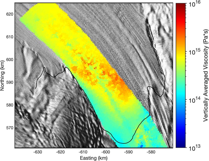
4108                                                                      A. Humbert et al.: Ice shelf melt channel evolution

   Surface troughs on ice shelves are linked to incisions at       rates. Besides seasonal variability, melt rates also change
the ice base, thus either to melt channels (e.g., Le Brocq         within smaller periods. Vaňková et al. (2020) identified melt
et al., 2013; Langley et al., 2014) or to basal crevasses (e.g.,   rate variations at the semi-diurnal M2 tidal constituent at 6 of
Humbert et al., 2015). The surface troughs are formed by           17 locations at Filchner–Ronne Ice Shelf, Antarctica. Like-
viscoelastic deformations in the transition to buoyancy and        wise, Lindbäck et al. (2019) and Sun et al. (2019) found di-
buoyancy equilibrium itself. Channels at the ice base have         urnal and fortnightly melt variations at other Antarctica ice
been surveyed using radio echo sounding (Rignot and Stef-          shelves. In situ observations of melt rates in sub-ice-shelf
fen, 2008; Vaughan et al., 2012; Le Brocq et al., 2013;            channels are often conducted with a phase-sensitive radio
Dutrieux et al., 2014; Langley et al., 2014; Dow et al., 2018).    echo sounder (pRES), which is described in more detail be-
Their typical dimensions range from 300–500 m wide and             low.
up to 50 m high (Langley et al., 2014) to 1–3 km wide and             Modeling basal melt rates adequately requires fully cou-
200–400 m high (Rignot and Steffen, 2008). Channel flanks          pled ice–ocean models that evaluate the energy balance at the
are not necessarily smooth but may form terrace structures in      ice–ocean transition to compute basal melt rates. While none
the lateral (across ice flow) dimension as shown by Dutrieux       of the global circulation models deals with ice shelf cavi-
et al. (2014) for Pine Island Glacier, Antarctica. These ter-      ties, there are some coupled ice-sheet–ocean models simu-
races are separated by up to 50 m high walls with steep slopes     lating large-scale basal melt rates (Gwyther et al., 2020; Din-
between 40 and 60◦ .                                               niman et al., 2016; Jourdain et al., 2017; Seroussi et al., 2017;
   Hofstede et al. (2021a) found a basal channel on Support        Timmermann and Hellmer, 2013; Galton-Fenzi et al., 2012).
Force Glacier at the transition to the Filchner Ice Shelf at-      However, only a few of them incorporate melt channels as
tributed to the outflow of subglacial water. The channel in-       this requires very high horizontal resolution: Gladish et al.
creases in height close to the grounding line and widens           (2012) showed that channels confine the warm water and
downstream. Between 7 and 14 km from the grounding line,           stabilize the ice shelf by preventing melt on broader spatial
the flanks of the channel become steeper and terraces form         scales. This conclusion is affirmed by Millgate et al. (2013),
on its sides, which are sustained over 38 km from the ground-      who found that an increasing number of melt channels lead
ing line, but with decreasing height between 14 and 38 km.         to a decreasing overall mean melt rate. Our study will pro-
Within this distance, the height of the channel varies only        vide an observational data set of basal melt rates that allows
slightly from 170 to 205 m. This particular channel is the fo-     understanding these types of modeling results.
cus of this study.                                                    The change in geometry due to mechanical deformation is
   Basal melt rates inside a channel underneath Ross Ice           another important contribution to the evolution of basal chan-
Shelf, Antarctica, were found by Marsh et al. (2016) to be up      nels (Bassis and Ma, 2015; Wearing et al., 2021). The spa-
to 22.2 m yr−1 near the grounding line and only 2.5 m yr−1         tial gradients in displacement u lead to strain ε that causes a
for observations 40 km downstream. Outside of the channel,         change in ice thickness. This process is governed by the vis-
the melt rate was only 0.82 m yr−1 , demonstrating enhanced        coelastic nature of a Maxwell fluid for ice. While ice is react-
melt inside the channel compared to its surroundings. At Pine      ing purely viscously on long timescales, its behavior on short
Island Glacier, Antarctica, Stanton et al. (2013) found basal      timescales is elastic (Reeh et al., 2000; Gudmundsson, 2011;
melt rates of up to 24 m yr−1 and an across-channel variabil-      Sergienko, 2013; Humbert et al., 2015; Christmann et al.,
ity that they suggested to be related to channelized flow. The     2016; Schultz, 2017; Christmann et al., 2019). The transi-
decrease in channel melt rates with distance downstream is         tion from grounded to floating ice and short-term geometry
likewise described by Le Brocq et al. (2013). Buoyant fresh        changes due to basal melt or accumulation are examples of
water initially enhances basal melting inside the channel by       ice affected by the elastic response. Over timescales of years,
increasing the vigor of the turbulent plume at the ice base and    viscous creep becomes more relevant. As a consequence, the
entraining more ambient warm water (Jenkins and Doake,             geometry of melt channels needs to be modeled using vis-
1991). However, at some point the rising plume can become          coelastic material models based on a characteristic Maxwell
supercooled due to the falling pressure, which leads to the        time of 153 d (deduced in the model section) arising from
formation of frazil ice and freeze-on. This is a general feature   the material parameters used for this study. Until now, the
of the thermohaline circulation underneath ice shelves (e.g.,      viscoelastic nature of the evolution of basal channels was ne-
MacAyeal, 1984). Similar to Le Brocq et al. (2013), Marsh          glected as previous studies only consider viscous ice flow.
et al. (2016) assumed that the channel at Ross Ice Shelf is           In this study, we present in situ melt rates of a large melt
formed by the outflow of subglacial meltwater. Washam et           channel feature in the southern Filchner Ice Shelf at the
al. (2019) found high seasonal variability in basal melting        inflow from Support Force Glacier (SFG). Field measure-
within a channel at Petermann Glacier, Greenland. In sum-          ments and satellite-borne data provide constraints to inves-
mer, melt rates reached a maximum of 80 m yr−1 , whereas           tigate how this feature evolves using numerical modeling.
in winter, melt rates were below 5 m yr−1 . They suggested         In addition to the spatial distribution of basal melt, we an-
that increased subglacial discharge during summer strength-        alyze the temporal evolution of melt rates. We split this pa-
ens ocean currents under the ice, which drives the high melt       per into two main parts, starting with observations followed

The Cryosphere, 16, 4107–4139, 2022                                                    https://doi.org/10.5194/tc-16-4107-2022
A. Humbert et al.: Ice shelf melt channel evolution                                                                            4109

by a modeling section. We present the methodology and the             We followed Brennan et al. (2014) and Stewart et al.
results in each part separately. A synthesis then follows fo-      (2019) for data processing to get amplitude- and phase-depth
cusing on the evolution of the melt channel.                       profiles. The final profile that contains the amplitude and
                                                                   phase information as a function of two-way travel time was
                                                                   obtained from a Fourier transformation. To convert two-way
2     Observations                                                 travel time into depth, the propagation velocity of the radar
                                                                   wave is computed following Kovacs et al. (1995). For this
2.1     Data acquisition                                           the vertical ice/firn density profile is required. Here we use
                                                                   a model described by Herron and Langway (1980). As input
We acquired data at a melt channel on the southern Filch-
                                                                   parameters, accumulation rate and mean annual temperature
ner Ice Shelf under the framework of the Filchner Ice
                                                                   are needed, for which we use data from the regional climate
Shelf Project (FISP). We performed 44 phase-sensitive radar
                                                                   model RACMO 2.3/ANT (van Wessem et al., 2014, multi-
(pRES) measurements (locations are shown in Fig. 1) in
                                                                   annual mean 1979–2011). Despite the correction of higher
the season 2015/16, which were repeated in 2016/17 as
                                                                   propagation velocities in the firn, the uncertainty of the ve-
Lagrangian-type measurements. These measurements were
                                                                   locity and thus of the depth is 1 % (Fujita et al., 2000).
taken in 13 cross-sections ranging from 14 to 61 km down-
stream from the grounding line (Fig. 1). This allows us to
investigate the spatial variability of basal melt rates. At each   2.2.2   Basal melt rates from repeated pRES
cross-section, up to four measurements were performed at                   measurements
different locations: at the steepest western flank (SW), at the
                                                                   The method for determining basal melting rates, previously
lowest surface elevation (L), at the steepest eastern flank (SE)
                                                                   described by, e.g., Nicholls et al. (2015) and Stewart et al.
and outside the east of the channel (OE; Fig. 1b). In order
                                                                   (2019), is based on the ice thickness evolution equation. The
to achieve an all-year time series, one autonomous pRES
                                                                   change in ice thickness over time ∂H /∂t consists of com-
(ApRES) station was installed (Fig. 1b). This instrument
                                                                   ponents arising from deformation and accumulation/ablation
performed autonomous measurements every 2 h, resulting in
                                                                   at both interfaces (e.g., Zeising and Humbert, 2021). As our
4342 measurements between 10 January 2017 and 6 January
                                                                   observations are discrete in time, the change in ice shelf
2018. One year earlier, a GPS station was also in operation
                                                                   thickness 1H within the time period 1t, which is caused
at this point from 24 December 2015 to 5 May 2016, the data
                                                                   by changes at the surface and in the firn 1Hs (e.g., snow
of which we use for tidal analysis. To distinguish the single
                                                                   accumulation/ablation and firn compaction), by strain in the
repeated measurements from the autonomous measurements,
                                                                   vertical direction 1Hε and by thickness changes due to basal
we refer to them as pRES and ApRES measurements, respec-
                                                                   melt 1Hb , is considered:
tively.

2.2     Materials and methods                                      1H   1Hs 1Hε 1Hb
                                                                      =    +    +                                                (1)
                                                                   1t   1t   1t   1t
2.2.1    pRES device and processing
                                                                   (Vaňková et al., 2020; Zeising and Humbert, 2021). In or-
The pRES device is a low-power, ground-based radar that            der to obtain the basal melt rate, the change in ice thickness
allows for estimating displacement of layers from repeated         must be adjusted for the other contributions. Snow accumu-
measurements with a precision of millimeters (Brennan et al.,      lation/ablation and firn compaction but also changes in radar
2014). This accuracy enables the investigation of even small       hardware or settings (a different pRES instrument was used
basal melt rates, taking into account snow accumulation to-        for the revisit) can cause a vertical offset near the surface that
gether with firn compaction and strain in the vertical di-         cannot be distinguished from one another. Following Jenk-
rection (Corr et al., 2002; Jenkins et al., 2006). The pRES        ins et al. (2006), we aligned both measurements below the
is a frequency-modulated continuous wave (FMCW) radar              firn–ice transition. To this end, we computed the depth at
that transmits a sweep, called chirp, over a period of 1 s         which pore closure takes place (hpc ), i.e., the depth at which
with a center frequency of 300 MHz and bandwidth of                a density of 830 kg m−3 is reached. We apply the densifica-
200 MHz (Nicholls et al., 2015). For a better signal-to-noise      tion model (Herron and Langway, 1980) and mean annual
ratio, the single repeated measurements were performed with        accumulation rate and temperature from the multi-year mean
100 chirps per measurement and the measurements of the             RACMO2.3 product (van Wessem et al., 2014). In our study
time series with 20 chirps due to memory and power limita-         area, hpc varies between 62 and 71 m. The actual alignment is
tions. After collecting the data, anomalous chirps within each     based on a correlation of the amplitudes for a window of 6 m
burst were removed, and the remaining chirps were stacked.         around hpc . No reliable alignment could be obtained from the
Anomalous chirps were identified by correlating each chirp         correlation for nine stations because the correlations of the
with every other chirp of the burst. Those with a low correla-     surrounding depths resulted in ambiguous alignments. As a
tion coefficient on average were rejected.                         consequence, these stations were not considered.

https://doi.org/10.5194/tc-16-4107-2022                                                  The Cryosphere, 16, 4107–4139, 2022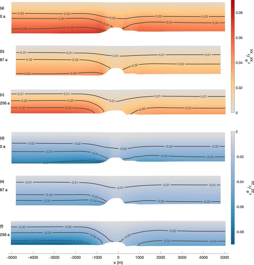
4110 A. Humbert et al.: Ice shelf melt channel evolution
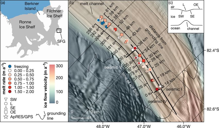
Figure 1. (a) Map of the Ronne and Filchner ice shelves. The study area near the Support Force Glacier (SFG) is marked with a black box.
(b) Study area with pRES-derived basal melt rates at 13 cross-sections of the melt channel. The different symbols indicate the position relative
to the channel, as shown in panel (c). Those melt rates derived from a nadir and an off-nadir basal return are marked with a white outline.
For each cross-section, the distance from the grounding line and the duration of ice flow from the location furthest upstream are given. The
location of an ApRES/GPS station is shown by a star. The seismic I, IV and V lines mark the location of active seismic profiles (Hofstede
et al., 2021a, b). The background is a hillshade of the Reference Elevation Model of Antarctica (Howat et al., 2018, 2019) overlaid by the
ice flow velocity (Hofstede et al., 2021a). (c) Sketch of a cross-section of the channel with measurement locations on the steepest western
surface flank (SW), at the lowest surface elevation (L), on the steepest eastern surface flank (SE) and outside the east of the channel (OE).
After the alignment, the change in the ice thickness Hi be- of 20 m below the surface to 20 m above the ice base. To
low the pore closure depth hpc is only affected by vertical determine vertical displacements, we cross-correlated each
strain and basal melt. Thus the basal melt rate ab (positive segment of the first measurement with the repeated mea-
for melting, negative for freezing) is surement. The lag of the largest amplitude correlation coeffi-
cient was used to find the correct minimum phase difference,
1Hb 1Hi 1Hε
ab = − =− − , (2) from which we derived the vertical displacement. Since noise
1t 1t 1t prevents the reliable estimation of the vertical displacement
with 1Hε being the thickness change due to vertical strain from a certain depth on, we calculated the depth at which the
obs . 1H is derived from integrating ε obs from the aligned
εzz ε zz
averaged correlation of unstacked chirps undercuts the em-
reflector at hpc to the ice base hb : pirical value of 0.65. We name this the noise-level depth limit
hnl , which is 743 m on average in this study area. Only those
Zhpc segments located below hpc and above hnl were used to avoid
obs densification processes and noise to influence the strain esti-
1Hε = εzz dz. (3)
mation. A linear regression was calculated from the shifts of
hb
the remaining segments, assuming a constant vertical strain
Here, hb denotes the average depth of the ice base of the distribution over depth as the overall trend. However, at six
measurements. The vertical strain is defined as stations, all in the hinge zone where the ice is bent by tides,
we observed a slight deviation from a linear trend at deeper
obs ∂uz
εzz = , (4) layers (Fig. A1a). A depth-dependent tidal vertical strain
∂z caused by tidal bending near the grounding line has been ob-
with the displacement in the vertical direction uz . served previously (Jenkins et al., 2006; Vaňková et al., 2020),
In order to determine uz , we followed the method de- although the long-term vertical strain was found to be depth-
scribed by Stewart et al. (2019). We divided the first measure- independent (Vaňková et al., 2020). The segments that indi-
ment in segments of 6 m width with 3 m overlap from a depth cate a non-linear distribution are located below hnl and are
The Cryosphere, 16, 4107–4139, 2022 https://doi.org/10.5194/tc-16-4107-2022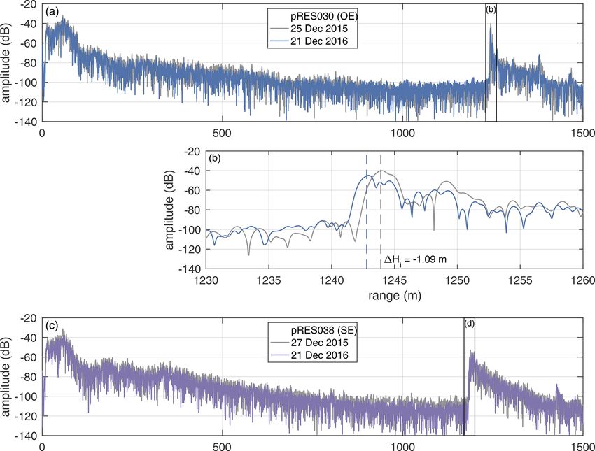
A. Humbert et al.: Ice shelf melt channel evolution                                                                                               4111

                                                                                                                                                  syn
hence not taken into account for the regression. Neverthe-                       We can invert this and calculate a synthetic melt rate ab (t)
less, we want to provide a lower limit of |1Hε | considering                     that reconstructs the observed ice thickness H :
other forms of strain-depth relations (Jenkins et al., 2006).
For this purpose, we use a strain model that is decreasing lin-                                      Zt
                                                                                                                                     syn
                                                                                                          1Hs (t 0 ) + 1Hε (t 0 ) + ab (t 0 ) dt 0 . (6)

early from half the ice thickness (approximately hnl ) to the                    H (t) = H (t0 ) +
depth of at which εzzobs = 0 (Fig. A1b). This serves as a lower                                      t0
                                    obs (z) gives the upper limit.
limit of |1Hε |, whereas a linear εzz
The average of both gives 1Hε and the difference the uncer-                      Descriptions of the symbols are given in Table A2.
tainty.
   In order to derive 1Hi , we used a wider segment of 10 m                      2.2.4   Basal melting from ApRES time series
around the basal return, which was identified by a strong in-
                                                                                 The processing of the autonomous measured time series with
crease in amplitude. Its upper limit is located 9 m above the
                                                                                 a 2 h measurement interval differs slightly from the single
basal return, while the lower limit is defined 1 m below the
                                                                                 repeated measurements. For the ApRES time series, the in-
basal return. The vertical displacement of the ice base and
                                                                                 strument was located below the surface, thus snow accumu-
thus the change in ice thickness was obtained from the cross-
                                                                                 lation had no influence on the measured ice thickness and an
correlation of the basal segment. However, more than one
                                                                                 alignment of the measurements is not necessary. This gives
strong basal reflection occurred at seven sites. For these sites,
                                                                                 the possibility to determine the firn compaction 1Hf . With-
we averaged the melt rates we derived from both basal seg-
                                                                                 out the alignment, thickness change due to strain needs to be
ments. In Appendix A1 we discuss the identification of the
                                                                                 considered for the whole ice thickness H :
basal reflection and the influence of off-nadir basal returns
on the estimation of basal melt rates (Table A1, Figs. A2 and                            ZH
A3).                                                                             1Hε =         obs
                                                                                              εzz  dz.                                              (7)
   The uncertainty of the melt rate results mainly from the
                                                                                         0
alignment of the repeated measurement and the uncertainty
of 1Hε . This leads to uncertainties in the melt rate of up to                   For processing, we followed the method described by Zeising
0.26 m yr−1 for locations in the hinge zone, while at other                      and Humbert (2021), which differs slightly from the process-
locations the uncertainty is predominantly in the range of                       ing applied by Vaňková et al. (2020). Similar to processing of
< 0.05 m yr−1 . At those stations where the melt rate was av-                    the single repeated measurements, we divided the first mea-
eraged, the error represents the difference of the two melt                      surement into the same segments and calculated the cross-
rates. Since this difference is up to 1.34 m yr−1 , the error sig-               correlation of the first measurement (t1 ) with each repeated
nificantly exceeds 0.26 m yr−1 in some cases.                                    measurement (ti ). The displacement was obtained by the lag
                                                                                 of the minimum phase difference. To avoid half-wavelength
2.2.3   Benchmarking melt rates and thickness evolution                          ambiguity due to phase wrapping, we limited the range of ex-
                                                                                 pected lag based on the displacement derived for the period
In order to classify how representative the melt rates are for                   t1 –ti−1 .
the past, we reconstructed the ice thickness based on the                            The estimation of the vertical strain for the period t1 –ti is
values derived from the pRES measurements. First, we lin-                        based on a regression analysis of the vertical displacements
early interpolated ab , 1Hε and 1Hs along the distance of the                    for chosen segments. Only those segments located below a
channel to get continuous values between the cross-sections                      depth of 70 m and above the noise-level depth limit of
and smoothed the results in order to obtain a trend for each                     h ≈ 600 m were used to avoid densification processes and
process. We converted the distance from the upstream-most                        noise influencing the strain estimation. Assuming constant
cross-section to an age beyond this cross-section by assum-                      strain over depth, the regression analysis gives the vertical
ing the mean flow velocity is constant in time and space.                        strain, and the cumulative displacement uz (z) is
Next, we treat the change in ice thickness as a transport equa-                            obs
                                                                                 uz (z) = εzz  z + 1Hf ,                                            (8)
tion. To this end, we compute the advection of the ice thick-
ness along the flowline under present-day climate conditions
                                                                                 where the intercept at the surface is the firn compaction 1Hf .
(HPDadv ). For this we use interpolated functions of ab (t),
                                                                                 Similar to determination of 1Hi of the single repeated mea-
1Hε (t) and 1Hs (t). The expected ice thickness at HPDadv is
                                                                                 surements, we derived the change in ice thickness 1H for a
then the thickness at t0 = 0 years plus the cumulative change
                                                                                 wider segment of 10 m. The cumulative melt of the ApRES
in ice thickness:
                                                                                 time series was finally derived by

                         Zt                                                                     Zt
                                                                                                     1H (t 0 ) − 1Hε (t 0 ) − 1Hf (t 0 ) dt 0 .

                              1Hs (t 0 ) + 1Hε (t 0 ) + ab (t 0 ) dt 0 .

HPDadv (t) = H (t0 ) +                                                     (5)   1Hb (t) = −                                                        (9)
                         t0                                                                     t1

https://doi.org/10.5194/tc-16-4107-2022                                                                   The Cryosphere, 16, 4107–4139, 2022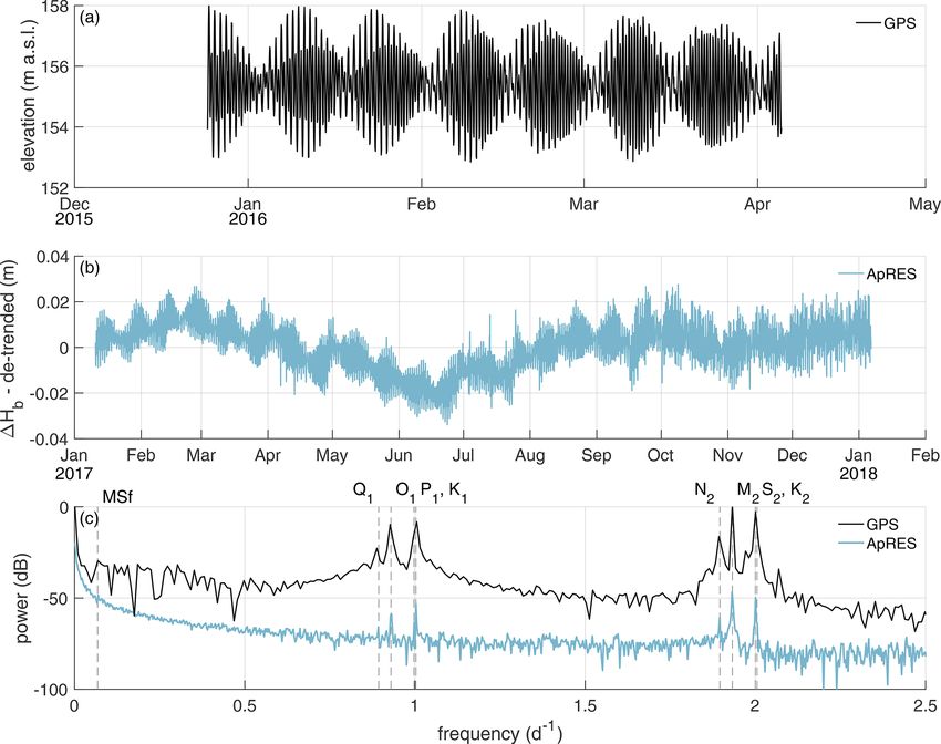
4112                                                                       A. Humbert et al.: Ice shelf melt channel evolution

In order to investigate if the basal melt is affected by tides,     At others, a change in the shape of the first basal return pre-
we first de-trended the cumulative melt time series and com-        vented the determination of the change in ice thickness.
puted the frequency spectrum afterwards.                               The estimated basal melt rates range from 0 to 2 m yr−1 ,
   Subsequently, we used the time series of 1H (t) to inves-        with the largest melt rates on the steepest western flank (SW)
tigate the occurrence of non-tidal melt events. We de-tided         of the channel (Fig. 2a). A trend of decreasing melt rates in
1H (t) twice – once by subtracting a harmonic fit based             the along-channel direction was found at the highest part (L)
on frequencies up to the fortnightly constituent (Mf) and           of the channel. Here, melt rates decrease from 1.8 m yr−1 to
secondly by subtracting a harmonic fit based on frequen-            basal freezing, measured at the three most downstream cross-
cies up to the solar annual constituent (Sa) to remove all          sections. Outside of the channel (OE), basal melt rates are
tide-induced signals and to calculate the thinning rate af-         more variable without a trend. Stations at the eastern flank
terwards. In this way, we identify non-tidal melt events and        (SE) show a lower range of variability. Here, ab varies be-
the influence of annual/seasonal signals without estimating         tween basal freezing and 0.8 m yr−1 .
the correct amount of strain thinning/thickening. Assuming             The height of the channel (difference in ice thickness be-
that basal melt causes changes on short timescales of sev-          tween L and OE; Fig. 2b) increases from about 200 m at the
eral days, we attribute abrupt increases in the thinning rate to    southernmost cross-section to a maximum of about 330 m
basal melt anomalies.                                               over a distance of 20 km in the ice flow direction. At this
                                                                    location, the melt rates within the channel fall below those
2.2.5    Global Positioning System (GPS) processing                 outside the channel and the height of the channel decreases,
                                                                    reaching ∼ 100 m at the northernmost cross-section.
The GPS processing is similar to the method used by Christ-            In Fig. 2c we display the melt rates as a function of ice
mann et al. (2021). With the Waypoint GravNav 8.8 pro-              shelf draft, derived from the TanDEM-X surface elevation
cessing software, we applied a kinematic precise point po-          and the pRES ice thickness. The melt rates outside the chan-
sitioning (PPP) processing for the GPS data that were stored        nel (OE) seem to be independent of the ice shelf draft, while
in daily files. We merged three successive daily solutions to       inside the channel (L) the melt rates decrease with reduced
enable full day overlaps avoiding jumps between individual          draft. However, melt rates at the largest draft inside the chan-
files. Afterwards, we combined the files in the middle of each      nel are approximately 3 times larger than those outside the
1 d overlap using relative point-to-point distances and re-         channel or at the steepest eastern flank (SE) at similar draft.
moved outliers. The data were low-pass filtered for frequen-           The distribution of 1Hε shows a significant thickening of
cies higher than 1/3600 Hz. For tidal analysis, we calculated       more than 1 m yr−1 at the most upstream cross-section at L
the power spectrum of the vertical displacement.                    and OE (Fig. A4). In the ice flow direction, 1Hε declines,
                                                                    reaching about zero above the channel at the cross-section
2.2.6    Digital elevation model (DEM)                              furthest downstream. In contrast, outside the channel, strain
                                                                    thinning occurred from 30 km downstream of the ground-
We use the TanDEM-X PolarDEM 90 m digital elevation                 ing line. The change in ice thickness due to firn compaction
data product provided by the German Aerospace Center                and accumulation is close to zero in the entire study area
(DLR) as reference elevation model (DLR, 2020). As the              (Fig. A4).
elevation values represent ellipsoidal heights relative to             However, the measurements only show a snapshot, as the
the WGS84 ellipsoid, we transform the PolarDEM to the               variability on longer timescales is unknown. Based on the in-
EIGEN-6C4 geoid (Foerste et al., 2014). In the following, we        terpolated melt rates, 1Hε and 1Hs along the channel (solid
refer to the DEM heights above the geoid as observed surface        lines in Figs. 3a and A4), we computed the advected ice
elevation hTDX . The absolute vertical height accuracy of the       thickness under present-day climate conditions HPDadv (solid
PolarDEM is validated against ICESat data and given to be           lines in Fig. 3b). The comparison of HPDadv with the mea-
< 10 m (Rizzoli et al., 2017). For our region of interest, the      sured ice thickness (dashed lines) shows large differences of
accuracy is given to be < 5 m as shown in Fig. 16 of Rizzoli        up to 185 m above the channel. While the observed ice thick-
et al. (2017).                                                      ness decreases rapidly above the channel, HPDadv remains al-
                                                                    most constant. In contrast, no significant differences between
2.3     Results and discussion of observations                      the observed ice thickness and HPDadv can be identified out-
                                                                    side the channel. If the present-day melt rates were repre-
2.3.1    Spatial melt rate distribution around basal                sentative of the long-term mean, the channel would close
         channel                                                    within 250 years, as the difference in HPDadv above and out-
                                                                    side the channel reaches zero. However, since the channel
We were able to determine basal melt rates at 34 of the 44 sin-     still exists beyond the northern end of our study area, it can
gle repeated pRES measurements. At some of the excluded             be concluded that the melt rates in the channel must have
stations, low correlation values prevented the alignment at         been higher in the past. How large the melt rates must have
the firn–ice transition or the estimation of the vertical strain.   been on average can be deduced from the reconstruction of

The Cryosphere, 16, 4107–4139, 2022                                                    https://doi.org/10.5194/tc-16-4107-2022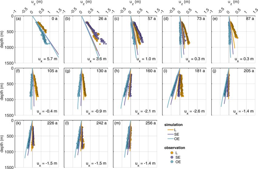
A. Humbert et al.: Ice shelf melt channel evolution 4113
Figure 2. Spatial distribution of pRES-derived (a) basal melt rates (positive ab represents melting) and (b) ice thickness at the locations SW
(red), L (yellow), SE (purple) and OE (blue) around the channel as a function of distance from the grounding line. (c) Melt rate as a function
of ice draft obtained from pRES-derived ice thickness and hTDX .
the existing ice thickness. The resulting synthetic average a few days and melted up to 1.5 cm of ice. In comparison, the
melt rate in the channel is about twice as high as the ob- annual or seasonal signals have little impact on the thinning
served melt rates, reaching 3.5 m yr−1 in the upstream area rate.
(yellow dashed line in Fig. 3a). Assuming a steady-state ice The unfiltered time series of the cumulative melt indicates
thickness upstream of the study area (supported by low eleva- a tidal signal with amplitudes of ∼ 1 cm within 12 h around
tion change found in Helm et al., 2014) and constant vertical the low-pass-filtered cumulative melt. However, we found
strain and accumulation in the past, this indicates that melt evidence that this tidal signal is due to the inaccuracy in the
rates in the last 250 years have been significantly higher than determination of the strain and not a true tidal melt ampli-
observed now. tude: we found a clear accordance of the strain in the upper
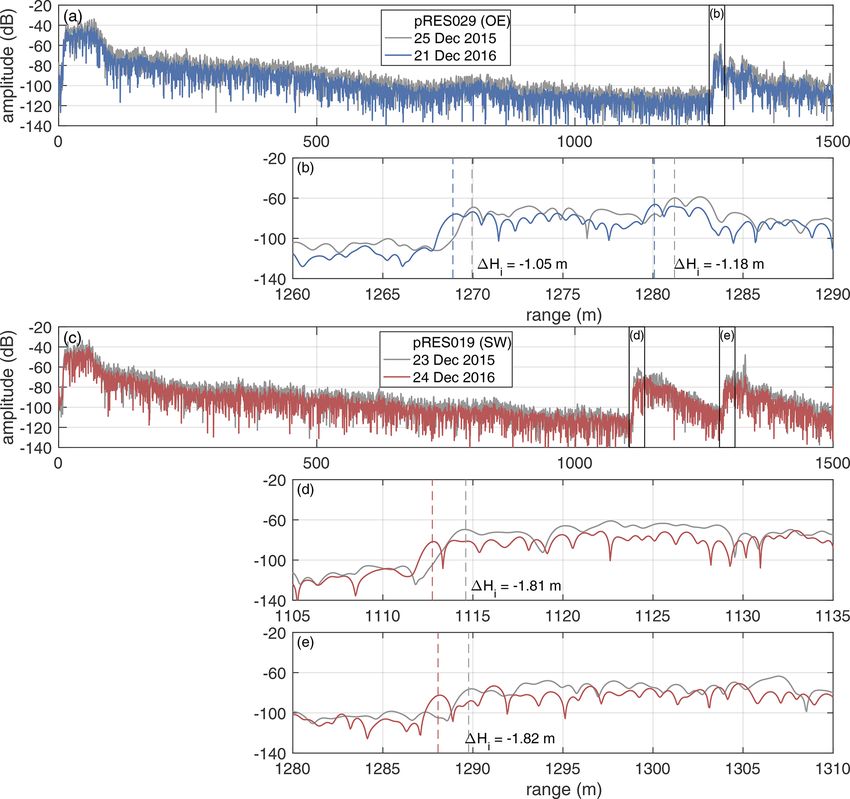
In addition to the observations we have presented in this ice column with the tidal signal as recorded by GPS mea-
section, we show the pRES-derived vertical displacement surements; however, we lack tidal vertical strain in the lower
profiles in Sect. 3.2.2 together with simulations. column of the ice due to the noise. As the tidal variation of
1H /1t is by far lower than the observed 1Hε /1t, either
2.3.2 Time series of basal melting deformations in the upper and lower parts compensate for
each other or basal melt/freeze takes this role. We can ex-
The ApRES time series outside the melt channel reveals clude freezing, as we do not find jumps in the amplitude of
an average melt rate of 0.23 m yr−1 (Fig. 4a). A look at the basal return in the ApRES signal (Vaňková et al., 2021)
the monthly mean melt rates shows increased melt dur- over tidal timescales. Consequently, we infer that strain in the
ing the summer months (January, February and November, lower half compensates for that in the upper part and there is
December) in comparison with the winter season. In these only a small variation of basal melt on tidal timescales.
months the melt rates show values from more than 0.3 up to As our location is close to two hinge zones, upstream and
0.62 m yr−1 . The spectral analysis of the unfiltered cumula- west of the melt channel, only a full three-dimensional model
tive melt time series shows all main diurnal and semi-diurnal could shed light on the vertical strain in the lower part of
constituents, which is in accordance with the frequencies ob- the ice column. This is numerically costly for the required
served from the GPS station (Fig. A5). non-linear strain theory and beyond the scope of the project.
The presence of the tide-induced signal prevents a robust With melt channels being located (or initiated) in the hinge
analysis of the basal melt rate as a high-resolution time se- zone, any kind of ApRES time series performed at thick ice
ries. Nevertheless, to investigate the occurrence of non-tidal columns might be affected by the unclear strain-depth profile
melt anomalies, we analyzed the time series of 1H (t) after it in the lower part of the ice column. This may be overcome
was de-tided. The resulting de-tided thinning rate shows sev- by a radar device with higher transmission power, which al-
eral melt anomalies distributed over the entire measurement lows the detection of vertical displacement of layers down to
period (Fig. 4b). These events lasted from a several hours to
https://doi.org/10.5194/tc-16-4107-2022 The Cryosphere, 16, 4107–4139, 2022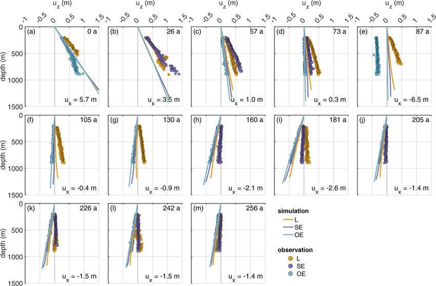
4114                                                                             A. Humbert et al.: Ice shelf melt channel evolution

Figure 3. (a) Melt rates at locations L (yellow) and OE (blue) are shown by dots (L) and squares (OE). The interpolated melt rates (ab ) are
                                                 syn
shown by solid lines, and synthetic melt rates (ab ) that are necessary to reproduce HpRES at L and OE are shown by dashed lines. (b) Ice
thicknesses at locations L (yellow) and OE (blue) are shown by dots (L) and squares (OE). The interpolated ice thicknesses (HpRES ) are
shown by dashed lines, and the advected ice thicknesses under present-day climate conditions (HPDadv ) from the observed melt rates at L
and OE are shown by solid lines. The two x axes show the distance from the grounding line in kilometers and the duration of ice flow in years
from the measurement location furthest upstream. Unconsidered observations were marked as outliers. Error bars mark the uncertainties of
the pRES-derived values.

Figure 4. Time series of basal melting at the ApRES location outside the channel. (a) Cumulative melt (blue line, left y axis) over the
measurement period from 10 January 2017 to 6 January 2018 with low-pass-filtered time series (black line). In September 2017, a malfunction
of the ApRES caused a change in the attenuation which resulted in a noisier time series. Monthly mean melt rates are shown by red lines
on the right y axis. Due to the inaccuracy in the determination of the strain, the cumulative melt still contains a contribution from strain.
(b) Thinning rate after subtracting of the tidal signal up to the fortnightly constituent (yellow line) and up to the solar annual constituent
(blue line). The dashed gray lines in panels (a) and (b) mark stronger melt events.

The Cryosphere, 16, 4107–4139, 2022                                                            https://doi.org/10.5194/tc-16-4107-2022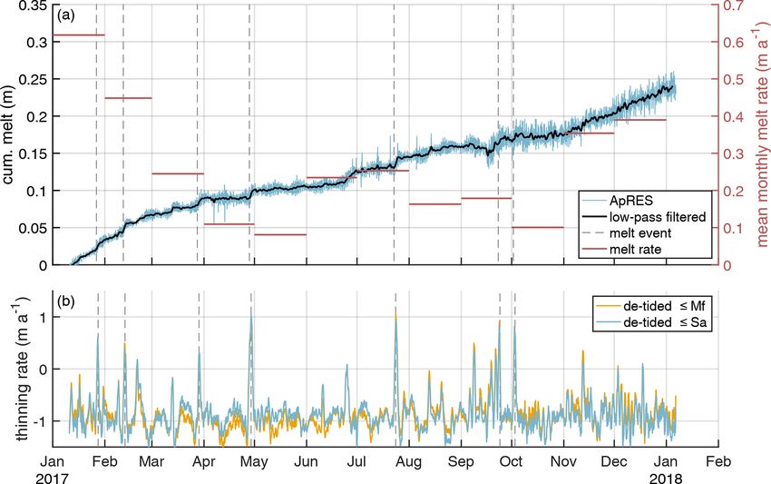
A. Humbert et al.: Ice shelf melt channel evolution                                                                          4115

the base. The observed tidal dependency of the vertical strain     ν). We conduct all viscoelastic simulations with commonly
is consistent with the finding from other ApRES locations at       used values for ice of E = 1 GPa and ν = 0.325 (Christmann
the Filchner–Ronne Ice Shelf by Vaňková et al. (2020). They       et al., 2019). Another material parameter of the viscoelas-
found the strongest dependency, even of the basal melt rate at     tic Maxwell material is the viscosity. It controls the viscous
some stations, on the semidiurnal (M2 ) constituent. Besides       flow of ice. We use a constant viscosity of η = 5 × 10¹⁵ Pa s
depth-independent tidal vertical strain, Vaňková et al. (2020)    and discuss the influence of this material parameter later
found tidal deformation from elastic bending at ApRES sta-         on. This constant viscosity is at the upper limit of the vis-
tions located near grounded ice.                                   cosity distribution derived by an inversion for the rheolog-
   For an ice shelf such as the Filchner we expect the prin-       ical rate factor in the floating part of the Filchner–Ronne
cipal drivers of basal melting to be the water speed and its       Ice Shelf (Sect. B2 and Fig. B2). This inversion has been
temperature above the in situ freezing point (e.g., Holland        conducted using the Ice-sheet and Sea-level System Model
and Jenkins, 1999). For much of the ice shelf the water speed      (ISSM) (Larour et al., 2012) in the higher-order Blatter–
is dominated by tidal activity (Vaňková et al., 2020), but near   Pattyn approximation (Blatter, 1995; Pattyn, 2003), using
the grounding line of SFG we expect the tidal currents to be       BedMachine geometry (Morlighem, 2020; Morlighem et al.,
low, consistent with the evidence from the ApRES thinning          2020), the velocity field of Mouginot et al. (2019b, a), and
rate time series. It is likely that the anomalously high melting   a temperature field presented in Eisen et al. (2020), based
events seen in the record result from the passage of eddies,       on the geothermal heat flux of Martos et al. (2017). For
with their associated water speed and temperature anomalies.       the assumed material parameters, we obtain a characteris-
                                                                   tic Maxwell time of τ = 153 d by τ = (2 + 2ν)η/E (Haupt,
                                                                   2000).
3     Viscoelastic modeling                                           The model geometry represents a cross-section through
                                                                   the melt channel (Fig. 5), with the x direction being across
To obtain a more profound understanding of the evolution           channel and resembling the seismic IV profile (Fig. 1) for
of the channel, we conduct transient simulations and analyze       t = 0 year. By assuming plane strain, the shape and the load-
the change in geometry of 2D cross-sections (x, z direction)       ing do not vary in the along-flow direction (width is suffi-
over time, as well as the simulated strain field. The simula-      ciently large). The stress state is independent of the third di-
tions are forced with the basal melt rates (both interpolated      mension, the displacement uy in the flow direction is zero
and synthetic) obtained in this study (Fig. 3). We transform       and hence all strain components in the direction of the width
distance (y direction) to time in the along-flow direction of      vanish:
the ice shelf (Fig. 1) using present-day velocities. This en-
ables us to study under which conditions the channel is stable     εyy = εxy = εyz = 0.                                       (10)
or vanishes.
   Ideally, we would have observations of ice geometry and
basal melt rates from the grounding line onward, but our first     The computational domain is discretized by an unstructured
cross-section with observations is located 14 km downstream        mesh using prisms with a triangular basis involving a re-
of the grounding line (Fig. 1). The initial elastic response of    fined resolution near the channel. We use the direct MUMPS
the grounded ice becoming afloat has faded away. Further           solver and backward differentiation formula with automatic
elastic contributions to the deformation originate from in situ    time step control and quadratic Lagrange polynomials as
melt at the base and accumulation at the surface. To best fit      shape functions for the displacements. The viscous strain is
the stress state at the first cross-section, we conduct a spin-    an additional internal variable in the Maxwell model, and we
up.                                                                use shape functions of the linear Lagrange type. In some
                                                                   cases, the geometry evolution leads to degraded mesh el-
3.1    Model                                                       ements, which requires automated remeshing from time to
                                                                   time.
The model comprises non-linear strain theory, as there is             In this study, the ice density is 910 kg m−3 and the seawa-
no justification to expect a priori the simplified, linearized     ter density is 1028 kg m−3 . At the upper and lower bound-
strain description for simulation times longer than 200 years      aries, we apply stress boundary conditions: for the ice–ocean
(e.g., Haupt, 2000). We treat the ice as a viscoelastic fluid      interface, a traction boundary condition specifies the wa-
and solve the system of equations for displacements using          ter pressure by a Robin-type condition. The ice–atmosphere
the commercial finite-element software COMSOL (Sect. B1;           interface is traction-free. Laterally, we apply displacement
Fig. B1; Christmann et al., 2019). The constitutive rela-          boundary conditions. As we take a plane strain approach, we
tion corresponds to a Maxwell material with an elastic re-         can neglect deformation in the along-flow direction. To ob-
sponse on short timescales and viscous response on long            tain realistic lateral boundary conditions, we transform ob-
timescales. For homogeneous, isotropic ice, two elastic mate-      served vertical strain and, hence, vertical displacements at
rial parameters exist (Young’s modulus E and Poisson’s ratio       the location OE in horizontal displacements. First, we as-

https://doi.org/10.5194/tc-16-4107-2022                                                 The Cryosphere, 16, 4107–4139, 2022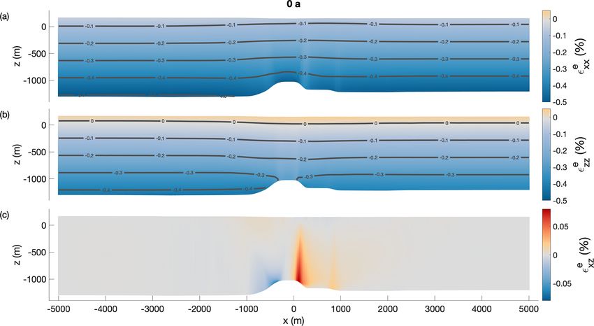
4116                                                                      A. Humbert et al.: Ice shelf melt channel evolution

sume incompressibility,

 obs      obs    obs
εzz  = − εxx  + εyy    ,                                   (11)

and compute the sum of the horizontal strain. We integrate
this strain to get a horizontal displacement. Therefore, we
assume a homogeneous material, no additional forces in the
horizontal direction and a constant ice thickness. The last as-
sumption is not valid inside the channel. However, with a
channel of 300 m maximum height over 1 km width, the devi-
ation from outside to inside the channel is small for a compu-
                                                                   Figure 5. The cross-section of the model geometry at the end of the
tational domain of around 10 km width and an ice thickness
                                                                   spin-up (t0 ) of the first experiment shows its corresponding width
around 1300 m. With these assumptions we get a constant            and ice thickness outside the east of the channel. The boundary con-
strain and integrate this strain to get a horizontal displace-     ditions of the viscoelastic model are the water pressure pw acting
ment. As we additionally assume plane strain, we can only          perpendicular to the ice base; the displacement in the flow direction
apply this displacement to the lateral boundary in the across-     uy , which is zero due to plane strain assumptions; and the time-
flow direction. To model the compression and extension of          dependent displacement ux (t) acting in the lateral direction derived
the ice flow through the embayment, we apply the horizontal        by pRES observations. The locations of the pRES station at the low-
displacement to each lateral side so that ux becomes               est point (L) of the channel and outside the east (OE) of the channel
                                                                 are shown at their position on the surface in addition to the SMB
         ZW                      ε obs + ε obs W                  (mass increase) and the melt rate ab (mass decrease) at the base of
       1      obs    obs
                                  xx      yy
                                                                   the geometry.
ux =         εxx  + εyy    dx =                   ,        (12)
       2                                 2
        0

with W the width of the simulated cross-section (Fig. 5).          is higher than outside the west of the channel, whereas after-
We assume that the horizontal displacements are depth-             wards the melt rates in the western part are higher than in the
independent at lateral boundaries, resulting in a compression      eastern part outside the channel.
or elongation perpendicular to the channel (Fig. B3a).                As we conduct Lagrangian experiments, we computed the
   The climate forcing consists of surface mass balance            time between the observed measurements through their dis-
(SMB) and basal melt rate. Technically, both are applied           tance divided by flow velocity. We define t0 = 0 year at the
by changing the geometry of the reference configuration            pRES measurements furthest upstream (Fig. 1) that is also
with the respective cumulative quantities (Fig. B3b, c). For       the location of the seismic observation IV by Hofstede et
the SMB, we used multi-year mean RACMO2.3 data (van                al. (2021a, b). To evaluate our simulations, we compare the
Wessem et al., 2014) ranging from 0.15 to 0.17 m yr−1 for          simulated surface topography and ice thickness as well as
a density of 910 kg m−3 , which we slightly modified to ac-        uz (z) with the observed one for the considered time interval
count for the surface depression over the channel: accumula-       of 250 years.
tion measurements at the pRES locations indicated higher ac-          We performed a spin-up to avoid model shocks, introduced
cumulation in the channel than outside by a factor of roughly      by the transient behavior of a Maxwell material, that could be
1.5. Thus, we used 50 % higher accumulation rates above the        falsely interpreted as the response to geometry changes, for
basal channel and a smooth cosine-shaped transition in the         instance, caused by basal melt rates. The main goal here is
x direction. A crucial forcing is of course the basal melt rate.   to have the geometry after spin-up fit reasonably to the ge-
Here we conduct individual experiments that are based on           ometry measured at the seismic IV line (see Fig. 1) that we
our observed melt rates and their variations. As these data are    denote as time t0 . The spin-up covers 75 years, which corre-
spatially sparse, we need to interpolate those values in the       sponds to the time from the grounding line to that profile un-
across-channel (x) direction. We assume a smooth cosine-           der present-day flow speeds. To this end, we take a constant
shaped transition between the observed basal melt rates out-       melt rate equal to the melt rate at t0 and adjust the geometry
side the east of the channel (OE) and inside the channel (L).      at the grounding line to match the geometry at t0 of the seis-
For melt rates outside the west of the channel, we do not have     mic IV profile reasonably well. After the spin-up, the width
any observations and assume them to be time-independent.           W (t0 ) of the simulated geometry is 10 km. With this proce-
With 10 % lower melt rates than for OE during the spin-up          dure the initial elastic deformation at the beginning of the
and a smooth cosine-shaped transition between outside the          transient simulation vanished and the viscoelastic geometry
west of the channel and the lowest surface elevation, we get a     evolution of the melt channel can be evaluated for different
good agreement of the ice base geometry for outside the west       melt scenarios and SMB forcings.
of the channel with seismic IV and V. For the first 20 years          Short-term forces like the time-varying climate forcing as
after the spin-up, the melt rate outside the east of the channel   well as the lateral extension or compression demand the us-

The Cryosphere, 16, 4107–4139, 2022                                                     https://doi.org/10.5194/tc-16-4107-2022
A. Humbert et al.: Ice shelf melt channel evolution 4117
age of a viscoelastic instead of a viscous model to simulate than the observed melt rate. Again, the melt rate has been
syn
the temporal evolution of the basal channel shown later on. kept constant over the spin-up with ab (t0 ). The synthetic
First, we conduct a series of simulations with different mate- melt rate leads to a cumulative melt after 250 years of 290 m
rial parameters and identify the best match of observed and (Fig. B3a), with 184 m more ice melted at L than in the first
simulated ice thickness above (L) and outside the east (OE) experiment, and, hence, the initial geometry has to be differ-
of the channel. At these two positions, most of the pRES ent to the first experiment; hence, we conduct an own spin-up
measurements were done, and the distribution of the melt simulation for the second experiment.
rates gives an adequate basis to force the model. Due to the The modeled geometry of this experiment is presented
sparsity of observations at the western side, we apply a forc- in Fig. 7. The simulated ice thickness at L is in very good
ing in the model based only on melt rates at L and OE. agreement with HpRES . There is some mismatch at OE, but
In the first experiment, we use an interpolation of the ob- the simulated trend of thinning is synchronous to the ob-
served melt rates as forcing and compare the results with servations. After 250 years the deviation from the observed
HPDadv (solid lines in Fig. 3). The second experiment aims to ice thickness at OE reaches +53 m. The simulated base
derive the best match between simulated and observed geom- for the second experiment shows a persistent basal channel
etry. For this experiment, we use synthetic melt rates (dashed (Fig. B5). The mismatch of the surface elevation at L and
lines in Fig. 3a). OE reverses over time: while the simulated surface topog-
raphy at OE is at first too low, it is too high in the second
3.2 Results and discussion of simulations half of the transient simulation (Fig. 7). However, the trends
of the observed hTDX and simulated hsim elevation behave
3.2.1 First experiment: pRES-derived melt rate similarly. While ice thickness is in good agreement, surface
elevation above the channel is overestimated by 4 m at the
The spin-up for this experiment starts with a manually ad- end of the spin-up. After 57 years, it turns from an overes-
justed geometry (including the channel at the base) at timation to an underestimation that results in an 8 m lower
t = −75 years to fit seismic IV profile at t0 . We applied a hsim than the observed hTDX after 250 years. To understand
constant melt rate of 1.5 m yr−1 at L and 0.5 m yr−1 at OE. if the ice is in hydrostatic equilibrium, we compute the free-
This forcing enlarges the melt channel during the spin-up as board at the position L for an ice density of 910 kg m−3 . The
the ice thickness OE increases due to the prescribed displace- surface elevation is 133 m at t0 and decreases to 112 m after
ment representing compression caused by the lateral bound- 250 years. Although hTDX is larger than this, the ice is ap-
aries moving towards the center of the channel. The general proaching flotation in the downstream direction. One could
shape of the base matches the seismic profile IV reasonably take another approach and estimate the mean density un-
well (Fig. 1 and Fig. B4). After the spin-up, we force the base der the assumption of buoyancy equilibrium: at t0 this cor-
with ab (solid line in Fig. 3a). responds to 901 kg m−3 , and after 250 years this corresponds
The results of this experiment are displayed in Fig. 6. For to 896 kg m−3 . As more ice is melted from below and with
both locations, L and OE, the simulated geometry and ob- higher snow accumulation at L, the density decreases, which
served geometry differ significantly. The simulated ice thick- is to be expected.
ness above the channel declines by 21 m in 250 years, while After 250 years, the simulated freeboard at L is 1 m higher
the observed thickness is 191 m thinner. Outside the chan- than the surface elevation of 138 m inferred by buoyancy
nel, the simulated trend shows thinning. This thinning begins equilibrium using an ice density of 910 kg m−3 , and at OE
after 50 years, whereas we find continuous thinning in the the discrepancy is 3 m. Overall, we see convergence to equi-
observations. This delayed onset of thinning is also repre- librium state at OE and the simulated surface elevation at L.
sented in the simulated surface topography. Most notable is At the end of the simulation, only hTDX above the channel
the match between simulated Hsim and advected HPDadv ice does not reach buoyancy equilibrium, which leads to the jus-
thickness under present-day climate conditions at the center tifiable assumption that the mean ice density at L is lower
of the channel (L). At the same time, the mismatch to HpRES than OE.
confirms that present-day melt rates would not lead to the At the position of the furthest upstream pRES observa-
observed channel evolution over 250 years. tions, we know from interferometry shown in Hofstede et
al. (2021a) that the location is still in the hinge zone. The
3.2.2 Second experiment: synthetic melt rate assumption of buoyant equilibrium is therefore likely to be
flawed. At the end of the simulation, the geometry should
The spin-up for the second experiment starts with a differ- be close to buoyancy equilibrium despite melting and a 50 %
ent geometry than the first experiment as the basal melt rate higher SMB at L than OE. Hence, simulations carried out us-
is different. However, it has also been manually adjusted ing a higher SMB within the channel would result in better
at t = −75 years to fit seismic IV profile at t0 . In the sec- agreement with the observed values of hTDX .
ond simulation experiment, we force the base with the syn- Next, we consider the variation of the vertical displace-
thetic melt rate (Fig. 3a) that is larger inside the channel ment with depth. The results are presented in Fig. 8. For
https://doi.org/10.5194/tc-16-4107-2022 The Cryosphere, 16, 4107–4139, 20224118 A. Humbert et al.: Ice shelf melt channel evolution Figure 6. First experiment: simulated surface elevation (a) and ice thickness (b) using the pRES-derived melt rate. Colors denote quantities above the channel (yellow) and outside the channel (blue). (a) Simulated surface elevation hsim (solid lines) and observed hTDX (dashed lines). (b) Simulated ice thickness Hsim (solid lines), under present-day climate conditions advected HPDadv (dashed-dotted lines) and observed HpRES (dashed lines). Gray lines represent the spin-up. Figure 7. Second experiment: simulated surface elevation (a) and ice thickness (b) using the synthetic melt rate. Colors denote quantities above the channel (yellow) and outside the channel (blue). (a) Simulated surface elevation hsim (solid lines) and observed hTDX (dashed lines). (b) Simulated ice thickness Hsim (solid lines) and observed HpRES (dashed lines). Gray lines represent the spin-up. this purpose, we calculated the cumulative vertical displace- increasing distance from the grounding line. Given the com- ment in 1 year. For comparability, the vertical displacements plexity of the problem, the simulations show a reasonable due to accumulation and snow compaction were removed agreement with the observations. The best match is reached from the observed distributions. Most notably, we move from at OE, which is not that surprising. The generally good agree- a vertically extensive regime to a compressive regime with ment of the simulated displacements outside the channel The Cryosphere, 16, 4107–4139, 2022 https://doi.org/10.5194/tc-16-4107-2022
A. Humbert et al.: Ice shelf melt channel evolution                                                                         4119

comes from tuning ux at the lateral boundary to match uz           Mercer and Whillans ice streams into the Ross Ice Shelf
from the pRES measurements at OE. A schematic illustration         were 22.2 m yr−1 (Marsh et al., 2016). These values dropped
of first principal strains and their directions shows a closure    to below 4 m yr−1 over a distance of 10 km and reached
of the channel for lateral compression and simultaneously a        2.5 m yr−1 after 40 km. We also find that the melt rates de-
thickening of the ice shelf that is larger inside the channel      crease by a factor of 5 in the center of the channel over a
than outside (Fig. B6). For lateral extension, we conversely       distance of 11 km; however, this takes place between 14 and
get a thinning of the ice shelf that is smaller inside the chan-   25 km downstream of the grounding line. At the Ross Ice
nel than outside. Both simulated and observed vertical dis-        Shelf, the ratio between the melt rates inside the channel and
placement distributions show that the strain decreases from        1 km outside it is about 27, whereas we find only a factor of
L to OE (Fig. 8). The only exception here is t = 57 years,         3, with the distance between L and OE being 1.8 km.
where the vertical strain at SE is larger than the one at L,          Zeising et al. (2022b) presented pRES-derived basal melt
in the observations. While at 0 and 26 years the deviation         rates downstream of our study area. Roughly 40 km down-
of the simulated displacements between L and OE is small,          stream of the northernmost cross-section (∼ 200 years of ice
it increases afterwards. From 105 years, the simulated ver-        flow), these measurements show that the channel still ex-
tical displacements agree very well with those of the pRES         ists, but with a small height of ∼ 16 m. Inside the channel,
measurements, where a displacement distribution was deriv-         Zeising et al. (2022b) determined a melt rate ∼ 0.20 m yr−1
able at L and OE. The same comparison for the first experi-        lower than outside. The larger melt rates outside the channel
ment (Fig. B7) shows similar results, with significantly less      compared to inside are in agreement with the finding of our
pronounced differences between L and OE. Hence, the mis-           study. In general, the channel height declines, so the channel
match to the observed vertical displacements for this exper-       fades out. The channel diminishes because melt rates inside
iment using the measured melt rates is higher than for the         the channel fall below those outside the channel. The trend
second experiment with the synthetic melt rates.                   in vertical strain has only a minor contribution to this evolu-
   As the last point of this second experiment, we consider        tion. We thus do not find any evidence that such channels are
the influence of the viscosity on the evolution of the melt        a cause for instabilities of ice shelves as suggested by Dow
channel (Fig. B8). To reach the ice thickness of seismic IV,       et al. (2018).
the simulation applying the smallest viscosity needs a higher         One of the main findings of our study is that the present
initial channel at the beginning of the spin-up (Sect. B3). The    geometry can only be formed with considerable higher melt
channel thickness of the pRES measurement is modeled best          rates in the past (see Fig. 3). This finding is based on the
using a viscosity of 5 × 10¹⁵ Pa s. A 2-times-higher viscos-       assumption that the strain rates were in the past similar to
ity leads to a geometry where the ice is 42 m thinner in the       the present day and that melt on both flanks of the channel
center of the channel after 250 years, while a 5-times-lower       is similar. This is justified, as significant changes in strain
viscosity results in 116 m thicker ice above the channel due to    would require a change in the system that would cause other
more viscous flow into the channel. The simulated ice thick-       characteristics to change, like the main flow direction, for
ness OE is similar for all three different viscosities. The dis-   which we do not find any indication. However, in our setting,
tributions of vertical displacement with depth illustrate that     we are in a compressive regime. A similar assumption may
the difference between L and OE is larger for smaller vis-         not be possible at other locations.
cosity values (Fig. B9). Often the viscosity of 5 × 10¹⁵ Pa s         The pRES melt rate observations covered only 1 year.
fits quite well to obtain the observations by the simulation,      As the ocean conditions within the sub-ice shelf cavity are
but for some a slightly (Fig. B9a) or a considerably lower         known to respond to the ocean forcing from the ice front
viscosity (Fig. B9c) would be needed.                              (e.g., Nicholls, 1997), we would expected them to be subject
   We also conducted simulations to test with extreme high         to significant interannual variability. Underlying any inter-
melt rates along the steep slopes at the flanks, which did not     annual variability, a long-term reduction in basal melt rates
lead to a reasonable evolution of geometry of the channel,         would be the expected response to a reduction in production
and they are therefore not presented here.                         of dense shelf waters north of the ice front, resulting from
                                                                   a reduction in sea ice formation (Nicholls, 1997), which in
                                                                   turn results from a reduction in the southerly winds that blow
4   Discussion                                                     freshly produced sea ice to the north.
                                                                      A decrease in northward motion of sea ice has been ob-
First we aim to compare our findings with other measure-           served in the satellite record (e.g., Holland and Kwok, 2012),
ments inside a melt channel, which are unfortunately still         but no observation of sea ice trends over 250 years is avail-
very sparse, and we want to emphasize here that there is a         able to our knowledge. The modeling experiments by Naugh-
strong need for more of this type of observation in the fu-        ten et al. (2021) also find decreasing ice shelf basal melt
ture. We find that melt rates inside the channel are in gen-       rates. This reduction is therefore consistent with higher basal
eral rather modest, < 2 m yr−1 . Values retrieved at a chan-       melt rates in the past. However, our model results suggest
nel 1.7 km from the grounding line at the inflow of the            that the mismatch between the past melt rates needed to ex-

https://doi.org/10.5194/tc-16-4107-2022                                                 The Cryosphere, 16, 4107–4139, 2022
You can also read


