Non-Parametric Stochastic Sequential Assignment With Random Arrival Times
←
→
Page content transcription
If your browser does not render page correctly, please read the page content below
Proceedings of the Thirtieth International Joint Conference on Artificial Intelligence (IJCAI-21)

    Non-Parametric Stochastic Sequential Assignment With Random Arrival Times

             Danial Dervovic1 , Parisa Hassanzadeh1 , Samuel Assefa1 , Prashant Reddy1
                                          1
                                            J.P. Morgan AI Research
           {danial.dervovic, parisa.hassanzadeh, samuel.a.assefa, prashant.reddy}@jpmorgan.com

                          Abstract                                             ing [Morishita and Okumura, 1983] there is a need for fil-
                                                                               tering a stream of comparable examples that are too numer-
     We consider a problem wherein jobs arrive at ran-                         ous for exhaustive manual inspection, with the imperative of
     dom times and assume random values. Upon each                             maximising the value of inspected examples. We shall take an
     job arrival, the decision-maker must decide imme-                         abstract view of jobs arriving, each having an intrinsic value.
     diately whether or not to accept the job and gain                            To this end, we extend a problem first considered by [Al-
     the value on offer as a reward, with the constraint                       bright, 1974], in which jobs arrive according to a random pro-
     that they may only accept at most n jobs over                             cess and take on random nonnegative values. At each job ar-
     some reference time period. The decision-maker                            rival, the decision-maker must decide immediately whether or
     only has access to M independent realisations of                          not to accept the job and gain the value on offer as a reward.
     the job arrival process. We propose an algorithm,                         They may only accept at most n jobs over some reference
     Non-Parametric Sequential Allocation (NPSA), for                          time period. In [Albright, 1974], this problem is solved op-
     solving this problem. Moreover, we prove that the                         timally by way of a system of ordinary differential equations
     expected reward returned by the NPSA algorithm                            (ODE). Importantly, the job arrival process is assumed to be
     converges in probability to optimality as M grows                         known and admits a closed-form mathematical expression.
     large. We demonstrate the effectiveness of the al-                        Solving the resulting system of ODEs analytically quickly
     gorithm empirically on synthetic data and on public                       becomes impractical, even for trivial job arrival processes.
     fraud-detection datasets, from where the motivation                       We propose an efficient algorithm, Non-parametric Sequen-
     for this work is derived.                                                 tial Allocation Algorithm (NPSA), which allows one merely
                                                                               to observe M realisations of the job arrival process and still
1    Introduction                                                              recover the optimal solution, as defined by this solution of
In industrial settings it is often the case that a positive class              ODEs, with high probability. We empirically validate NPSA
assignment by a classifier results in an expensive manual in-                  on both synthetic data and public fraud data, and rigorously
tervention. A problem frequently arises whereby the number                     prove its optimality.
of these alerts exceeds the capacity of operators to manually                     This work plugs the gap in the literature where the follow-
investigate alerted examples [Beyer et al., 2016]. A com-                      ing must be simultaneously accounted for: i. explicit con-
mon scenario is one where each example is further endowed                      straints on the number of job acceptances; ii. maximising
with an intrinsic value along with its class label, with all                   reward; iii. treating job arrivals as a continuous-time random
negative examples having zero value to the operator. Given                     process; and iv. learning the job value distribution and arrival
their limited capacity, operators wish to maximise the cumu-                   process from data.
lative value gained from expensive manual interventions. As                    Related Work. The framework of Cost-sensitive learn-
an example, in financial fraud detection [Bolton and Hand,                     ing [Elkan, 2001] seeks to minimise the misclassification
2002], this is manifested as truly fraudulent transactions hav-                cost between positive and negative examples, even on an
ing value to the operator as (some function of) the mone-                      example-by-example basis [Bahnsen et al., 2014], but of-
tary value of the transaction, and non-fraudulent transactions                 ten the methods are tuned to a specific classification al-
yielding zero value [Dal Pozzolo, 2015].                                       gorithm and do not admit specification of an explicit con-
   In this paper we systematically account for the constraint                  straint on the number of positive labels. In [Shen and Kur-
on intervention capacity and desire to maximise reward, in                     shan, 2020], the authors formulate fraud-detection as an RL
the setting where selections are made in real-time and we                      problem. They explicitly take into account the capacity
have access to a large backlog of training data. This prob-                    of inspections and costs, but operate in discrete-time and
lem structure is not limited to fraud, for example in cy-                      provide no theoretical guarantees. Solving a Constrained
bersecurity [Vaněk et al., 2012], automated content mod-                      MDP [Altman, 1999] optimises reward under long-term con-
eration [Consultants, 2019], compliance verification [Aven-                    straints that can be violated instantaneously but must be sat-
haus et al., 1996] and automated inspection in manufactur-                     isfied on average, such as in [Efroni et al., 2020; Zheng and

                                                                        4214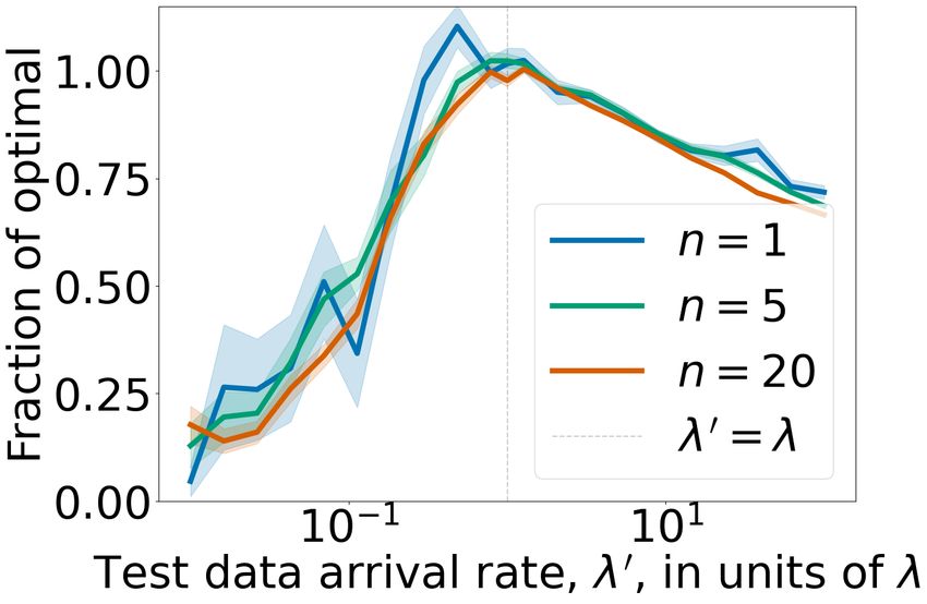
Proceedings of the Thirtieth International Joint Conference on Artificial Intelligence (IJCAI-21)

Ratliff, 2020]. Works such as [Mannor and Tsitsiklis, 2006;                     graph, that is, to derive critical curves for the n workers so
Jenatton et al., 2016] on Constrained Online Learning fo-                       as to maximise the expected cumulative reward at test time.
cus on a setting where the decision-maker interacts with an                     In Section 3.1 we present an efficient algorithm for deriving
adversary and is simultaneously learning the adversary’s be-                    these critical curves. We hereafter refer to the modified prob-
haviour and the best response, as measured by regret and vari-                  lem we address in this paper as Non-Parametric SeqAlloc, or
ants thereof [Zhao et al., 2020]. Constraints typically relate to               SeqAlloc-NP for short.
quantities averaged over sample paths [Mannor and Shimkin,
2004], whereas in our problem we have a discrete finite re-                     3     Optimal Sequential Assignment
source that is exhausted. In this work we consider a non-
adversarial environment that we learn before test-time from                     Following [DeGroot, 1970; Sakaguchi, 1977] we define a
training data. Moreover, the setting we focus on here explic-                   function that will take centre-stage in the sequel.
itly is continuous-time and finite horizon, contrasting with the                Definition 1 (Mean shortage function). For a nonnegative
constrained MDP and online learning literature which con-                       random variable X with pdf f and finite
                                                                                                                     R ∞ mean µ, the mean
siders discrete-time with an often infinite horizon. Our prob-                  shortage function is given as φ(y) := y (x − y)f (x) dx for
lem aligns most closely with the framework of Stochastic Se-                    y ≥ 0.
qential Assignment Problems (SSAP) [Derman et al., 1972;
                                                                                  The next result follows from [Albright, 1974, Theorem 2].
Khoshkhou, 2014], where it is assumed that distributions of
job values and the arrival process are known and closed-form                    Theorem 1 (SeqAlloc critical curves). The (unique) optimal
optimal policies derived analytically; the question of learning                 critical curves yn (t) ≤ . . . ≤ y1 (t) solving the SeqAlloc
from data is ignored [Dupuis and Wang, 2002].                                   problem satisfy the following system of ODEs (where 1 ≤
                                                                                k ≤ n):
2    Problem Setup                                                                        dyk+1 (t)
                                                                                                    = −λ(t) (φ(yk+1 (t)) − φ(yk (t))) ,
We follow a modified version of the problem setup in [Al-                                    dt
bright, 1974]. We assume a finite time horizon, from t = 0                               φ(y0 (t)) = 0,   yk (T ) = 0,     t ∈ [0, T ].
to t = T , over which jobs arrive according to a nonhomo-
geneous Poisson process with continuous intensity function                         Indeed, solving this system of ODEs exactly is generally
λ(t). There are a fixed number of indistinguishable work-                       intractable, as we shall see in more detail in Section 4. Theo-
ers, n, that we wish to assign to the stream of incoming jobs.                  rem 1 provides the optimal solution to the SeqAlloc problem.
Each worker may only accept one job. Every job has a non-
                                                                                3.1    Numerical Algorithm for SeqAlloc-NP
negative value associated to it that is gained as a reward by
the decision-maker if accepted. Any job that is not assigned                    An algorithm to solve the non-parametric problem,
immediately when it arrives can no longer be assigned. It is                    SeqAlloc-NP, immediately suggests itself as shown in
assumed the total expected number of jobs that arrive over                      Algorithm 1: use the M independent realisations of the job
the horizon [0, T ] is much larger than the number of available                 arrival process to approximate the intensity λ(t) and the
                        RT                                                      mean shortage function φ(y), then use a numerical ODE
workers, that is, n  0 λ(t) dt.
                                                                                solver with Theorem 1 to extract critical curves.
   We take the job values to be i.i.d. nonnegative random
variables drawn from a cumulative distribution F with finite
mean 0 < µ < ∞ and density f . Moreover, we assume that                          Algorithm 1: NPSA: solution to SeqAlloc-NP
the job value distribution is independent of the arrival process.                 Input: Number of workers n, ODE solver D
The decision-maker’s goal is to maximise the total expected                       Data: M realisations of job arrival process, M
reward accorded to the n workers over the time horizon [0, T ].                                            yk (t)}nk=1
                                                                                  Output: Critical curves {e
We hereafter refer to Albright’s problem as SeqAlloc (short                         begin
for Sequential Allocation).                                                                                   e from M
   In the SeqAlloc model, it is assumed that λ(t) and F are                            Estimate λ(t)e and φ(y)
known to the decision-maker ahead of time, and an optimal                              ye0 (t) ← ∞, Y ← {e     y0 (t)}
critical curve yk (t) is derived for each of the n workers.                            for k in (1, . . . , n) do
When the k th worker is active, if a job arrives at time t with                              Solve via D: yek (T
                                                                                                                ) = 0, t ∈ [0, T ].
                                                                                             de
                                                                                              yk (t)
value greater than yk (t) the job is accepted, at which point                                  dt    = −λ(t) φ(e
                                                                                                          e      e yk (t)) − φ(e
                                                                                                                             e yk−1 (t)) ,
the (k − 1)th worker is then active, until all n workers have                               Y ← Y ∪ {e   yk (t)}
been exhausted. These critical curves are addressed in more
detail in Theorem 1.                                                                    return Y \ ye0 (t)
   We modify the SeqAlloc problem setting in the following
way. The arrival intensity λ(t) and F are unknown to the
decision-maker ahead of time. Instead, they have access to                         Algorithm 1 is a meta-algorithm in the sense that the es-
M independent realisations of the job arrival process. Each                     timators λ(t)
                                                                                         e and φe must be defined for a full specification.
realisation consists of a list of tuples (xi , ti ), where xi is the            These estimators must be accurate so as to give the correct
reward for accepting job i and ti its arrival time. The goal                    solution and be efficient to evaluate, as the numerical ODE
for the decision-maker is the same as in the previous para-                     solver will call these functions many times. In Section 3.2

                                                                         4215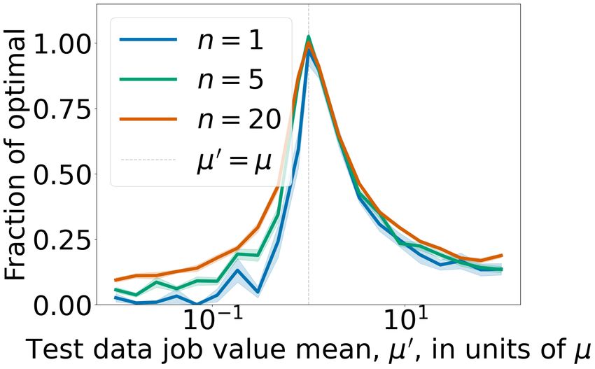
Proceedings of the Thirtieth International Joint Conference on Artificial Intelligence (IJCAI-21)

we define λ(t)
           e     and in Section 3.3 we define φe appropri-                      φi evaluated at each data sample xi and linearly interpolate
ately. Taken together with Algorithm 1 this defines the Non-                    for intermediate y ∈ [xi , xi+1 ) at evaluation time. Indeed,
parametric Sequential Allocation Algorithm, which we des-                       after initial one-time preprocessing, this estimate φeN (y) has
ignate by NPSA for the remainder of the paper.                                  a runtime complexity of O(log N ) per function call (arising
                                                                                from a binary search of the precomputed values) and space
3.2   Estimation of Non-Homogeneous Poisson                                     complexity O(N ), where N is the number of data samples
      Processes                                                                 used for estimation. Pseudocode for these computations is
In this section we discuss estimation of the non-homogeneous                    given in the Supplementary Material.
Poisson process P with rate function λ(t) > 0 for all t ∈                          We have shown that the NPSA mean-shortage function es-
[0, T ]. We make the assumption that we have M i.i.d. ob-                       timator is computationally efficient. It now remains to show
served realisations of this process. In this case, we adopt the                 that it is accurate, that is, statistically consistent.
well known technique of [Law and Kelton, 1991] specialised                      Theorem 3. Let X be a nonnegative random variable with
by [Henderson, 2003]. Briefly, the rate function estimator                      associated mean shortage function φ. Then, the estimate of
is taken to be piecewise constant, with breakpoints spaced                      the mean shortage function converges in probability to the
equally according to some fixed width δ.                                        true value, that is,
   Denote by λ  e(M ) (t) the estimator of λ(t) by M indepen-
dent realisations of P . Let the subinterval width used by the                                lim P sup φN (y) − φ(y) >  = 0
                                                                                                             e
estimator be δM > 0. We denote by Ci (a, b) the number of                                    N →∞        y≥0
jobs arriving in the interval [a, b) in the ith independent re-                 for any  > 0, where the estimate computed by the estimator
alisation of P . For t ≥ 0, let `(t) := bt/δM c · δM so that
                                                                                using N independent samples of X is denoted by φeN (y).
t ∈ [`(t), `(t) + δM ]. Our estimator is the number of arrivals
recorded within a given subinterval, averaged over indepen-                     Proof Sketch. It can be shown that an upper-
dent realisations of P and normalised by the binwidth δM ,                      bound on |φeN (y) − φ(y)|        is induced by an
that is,                                                                        upper-bound on |FN (x) − F (x)|.          The Dvoret-
                             M                                                  zky–Kiefer–Wolfowitz inequality [Dvoretzky et al., 1956;
         e(M ) (t) =    1 X                                                     Massart, 1990] furnished with this bound yields the
         λ                      Ci (`(t), `(t) + δM ).                (1)
                       M δM i=1                                                 result.
From [Henderson, 2003, Remark 2] we have the following                          3.4    NPSA Performance Bounds
result.                                                                         We have shown that the individual components of the NPSA
Theorem 2 (Arrival rate estimator convergence). Suppose                         algorithm, namely the intensity λ(t)
                                                                                                                   e and mean shortage φ(y)  e
that δM = O(M −a ) for any a ∈ (0, 1) and fix t ∈ [0, T ).                      estimators, are computationally efficient and statistically con-
      e(M ) (t) → λ(t) almost surely as M → ∞.
Then, λ                                                                         sistent. However, our main interest is in the output of the
                                                                                overall NPSA algorithm, that is, will following the derived
   For the NPSA algorithm we use Eq. (1) with δM =                              threshold curves at test time yield an expected reward that is
        1
T · M − 3 as the estimator for the intensity λ(t). There are                    optimal with high probability? The answer to this question is
dT /δM e ordered subintervals, so the time complexity of eval-                  affirmative under the assumptions of the SeqAlloc-NP prob-
uating λ(t)
       e     is O(log(T /δM )) and the space complexity is                      lem setup as described in Section 2.
O(T /δM ), owing respectively to searching for the correct                         We will need some results on approximation of ODEs. Fol-
subinterval [`(t), `(t) + δM ] via binary search and storing the                lowing the presentation of [Brauer, 1963], consider the initial
binned counts Ci . The initial computation of the Ci incurs a                   value problem
time cost of O(M Nmax ), where Nmax denotes the maximum                                                   dx
number of jobs over the M realisations.                                                                       = f (t, x),                      (2)
                                                                                                          dt
                                                                                where x and f are d-dimensional vectors and 0 ≤ t < ∞.
3.3   Mean Shortage Function Estimator                                          Assume that f (t, x) is continuous for 0 ≤ t < ∞, kxk < ∞
The following result (with proof in the Supplementary Mate-                     and k · k is a norm. Recall that a continuous function x(t)
rial) leads us to the φe estimator for NPSA.                                    is an -approximation to (2) for some  ≥ 0 on an interval
                                                                                if it is differentiable on an interval I apart for a finite set of
Lemma 1. The mean Rshortage function of Definition 1 can
                       ∞
be written as φ(y) = y (1 − F (x))dx, where F is the cdf                        points S, and k dx(t)
                                                                                                   dt − f (t, x(t))k ≤  on I \S. The function
of the random variable X.                                                       f (t, x) satisfies a Lipschitz condition with constant Lf on a
                                                                                region D ⊂ R × Rd if kf (t, x) − f (t, x0 )k ≤ Lf kx − x0 k
   Lemma 1 suggests the following estimator: perform the                        whenever (t, x), (t, x0 ) ∈ D. We will require the following
integral in Lemma 1, replacing the cdf F with the empiri-                       lemma from [Brauer, 1963].
cal cdf for the job value r.v. X computed with the samples
                                PN                                              Lemma 2. Suppose that x(t) is a solution to the initial value
(x1 , . . . , xN ), FN (x) := N1 i=1 1xi ≤x , where 1ω is the in-
                                                                                problem (2) and x0 (t) is an -approximate solution to (2).
dicator variable for an event ω. Since the empirical cdf is
                                                                                Then
piecewise constant, the integral is given by the sum of areas
of O(N ) rectangles. Concretely, we cache the integral values                      kx(t) − x0 (t)k ≤ kx(0) − x0 (0)keLf t +
                                                                                                                                Lf   (eLf t − 1),

                                                                         4216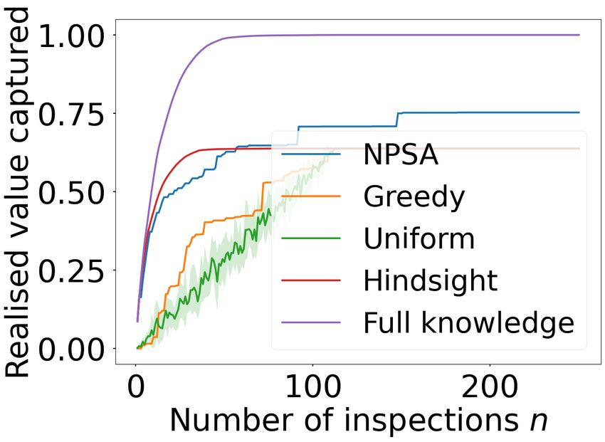
Proceedings of the Thirtieth International Joint Conference on Artificial Intelligence (IJCAI-21)

where Lf is the Lipschitz-constant of f (t, x).                                       We wish to lower-bound the expected total reward at test
   Now consider two instantiations of the problem setup with                       time using the thresholds {yk0 }nk=1 , when the job arrival pro-
differing parameters, which we call scenarios: one in which                        cess has value distribution F and intensity λ(t).
the job values are nonnegative r.v.s X with mean µ, cdf F                             We first make the assumptions that the functions H and
and mean shortage function φ; in the other, the job values are                     F do not differ too greatly between the critical curves
nonnegative r.v.s X 0 with mean µ0 , cdf F 0 and mean short-                       derived for the two scenarios. Concretely, there exist
age function φ0 . We stipulate that X and X 0 have the same                        F , δF , δH ∈ (0, 1) such that eδH H(yk (t)) ≥ H(yk0 (t)) ≥
support and admit the (bounded) densities f and f 0 respec-                        e−δH H(yk (t)), eδF F (yk (t)) ≥ F (yk0 (t)) ≥ e−δF F (yk (t))
tively. In the first scenario the jobs arrive with intensity func-                 and F (yk0 (t)) − F (yk (t)) ≤ F for all k ∈ {1, . . . , n}
tion λ(t) > 0 and in the second they arrive with intensity                         and t ∈ [0, T ]. Furthermore, we define the mean arrival rate
λ0 (t) > 0. In both scenarios there are n workers. We are to                                  RT
                                                                                   λ := T1 0 λ(t)dt. We are then able to prove the following
use the preceding results to show that the difference between                      lower bound on the total reward under incorrectly specified
threshold curves |yk (t) − yk0 (t)| computed between these two                     critical curves.
scenarios via NPSA can be bounded by a function of the sce-
nario parameters.                                                                  Lemma 5. Let δ = max {δH , δF }. Then
   We further stipulate that the scenarios do not differ by too
great a degree, that is, (1 − δλ )λ(t) ≤ λ0 (t) ≤ (1 + δλ )λ(t)                         En (t; yk0 , . . . , y10 ) ≥ e−n(δ+λF T ) En (t; yn , . . . , y1 ).
for all t ∈ [0, T ] and (1 − δφ )φ(y) ≤ φ0 (y) ≤ (1 + δφ )φ(y)                     Proof Sketch. Use induction on n and Eq. (4).
for all y ∈ [0, ∞), where 0 < δλ , δφ < 1. Moreover, define
λmax = maxt∈[0,T ] {λ(t)}. We are led to the following result.                        We have the ingredients to prove the main result. There is a
                                                                                   technical difficulty to be overcome, whereby we need to push
Lemma 3. For any k ∈                  {1, . . . , n}, yk0 (t) is     an -         additive errors from Lemma 4 through to the multiplicative
approximator for yk (t) when         > 2µλmax (δφ + δλ ).                         errors required by Lemma 5. This is possible when the func-
Proof Sketch. Upper bound the left-hand-side of                                    tions H, F and φ are S  all Lipschitz continuous and have pos-
                                                                                                             n
                                                                                   itive lower-bound on k=1 Range (yk (t)) ∪ Range (yk0 (t)),
 λ0 (t) φ0 (yk+1
             0
                 ) − φ0 (yk0 ) − λ(t) φ(yk+1
                                         0
                                             ) − φ(yk0 ) < ,

                                                                                   facts which are established rigorously in the Supplementary
where the ODE description of yk and yk0 is employed from                           Material.
Theorem 1 and use the definition of an -approximator.                                As a shorthand, we denote the expected reward gained by
                                                                                   using the optimal critical curves by r? := En (0; yn , . . . , y1 ).
  We are now able to compute a general bound on the differ-                        Moreover, let the critical curves computed by NPSA from M
ence between threshold curves derived from slightly differing                                                             (M )
                                                                                   job arrival process realisations be {eyk }nk=1 and the associ-
scenarios.                                                                         ated expected reward under the true data distribution be the
Lemma 4. For any k ∈ {1, . . . , n}                                                                                     (M )       (M )
                                                                                   random variable R(M ) := En (0; yen , . . . , ye1 ).
                                                                                   Theorem 4. Fix an arbitrary  ∈ (0, 1). Then,

      |yk (t) − yk0 (t)| ≤ (δλ + δφ )µ e2λmax (T −t) − 1 .
                                                                                                             (M )
                                                                                                              R
Proof Sketch. Compute the Lipschitz constant 2λmax for the                                          lim P           ≥ 1 −  = 1.
ODE system of Theorem 1, then use Lemmas 2 and 3.                                                  M →∞         r?

   Having bounded the difference between threshold curves in                       Proof Sketch. Using Lemma 5 one can lower bound the prob-
two differing scenarios, it remains to translate this difference                   ability by
into a difference in reward. Define
                                                                                                                         h         i
                                                                                       1 − P δH > 2            2              2

                 R∞                                                                                 n − P δF > n − P F > nλT .          (6)
       H(y) := y xf (x)dx;          F (y) := 1 − F (y), (3)
                                                                                   Lemma 4 and Theorem 3 can be used to show that the third
so that φ(y) = H(y) − yF (y) by Lemma 1. We also have                              term of (6) vanishes as M → ∞. The first and second term
from [Albright, 1974, Theorem 2] that for a set of (not nec-                       also vanish by pushing through the additive error from The-
                                    yk (t)}nk=1 , the expected
essarily optimal) threshold curves {e                                              orem 3 and Lemma 4 into multiplicative errors, then verify-
reward to be gained by replaying the thresholds from a time                        ing these quantities are small enough when M is sufficiently
t ∈ [0, T ] is given by                                                            large.
 Ek (t; yek , . . . , ye1 ) =                                                         Theorem 4 demonstrates that the NPSA algorithm solves
   Z T                                                                           the SeqAlloc-NP problem optimally when the number of re-
            H(e                 yk (τ )) · Ek−1 (τ ; yek−1 , . . . , ye1 )
                  yk (τ )) + F (e                                                  alisations of the job arrival process, M , is sufficiently large.
     t

                               Rτ
              × λ(τ ) exp − t λ(σ)F (e

                                              yk (σ))dσ dτ. (4)                    4    Experiments
                                                                                   We now empirically validate the efficacy of the NPSA algo-
We also have from [Albright, 1974, Theorem 1] that                                 rithm. Three experiments are conducted: i. observing the
                                         Pn                                        convergence of NPSA to optimality; ii. assessing the impact
             En (t; yen , . . . , ye1 ) = k=1 yek (t)                    (5)       on NPSA performance when the job value distribution F and

                                                                            4217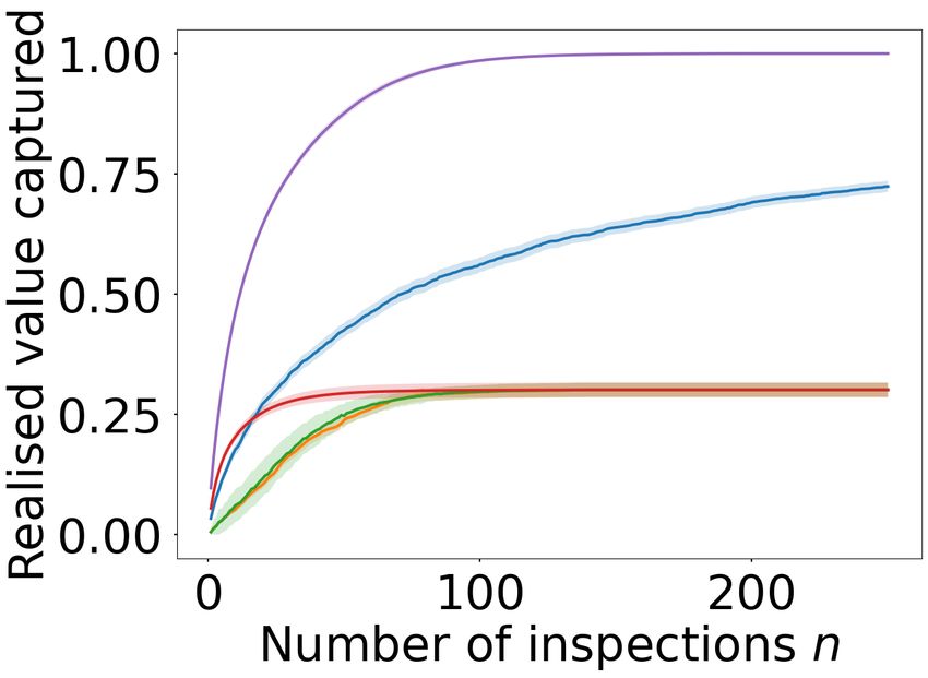
Proceedings of the Thirtieth International Joint Conference on Artificial Intelligence (IJCAI-21)
Using the SageMath [The Sage Developers, 2020] inter-
face to Maxima [Maxima, 2014], we are able to symbolically
solve for the optimal thresholds (using Theorem 1) when
n ≤ 20 for exponentially distributed job values and n = 1
for Lomax-distributed job values. P The optimal reward r? is
n
computed using the identity r? = k=1 yk (0) from (5). We
then simulate the job arrival process for M ∈ {1, . . . , 100}
independent realisations. For each M , NPSA critical curves
Figure 1: Convergence experiments for job values that are exponen- are derived using the M realisations. Then, using the same
tially distributed (left) with mean µ = 5 and job values that are data-generating process M 0 = 50 independent realisations
Lomax-distributed (right) with shape α = 3.5 and scale ξ = 5. The are played out, recording the cumulative reward obtained.
time horizon T = 2π and the job arrival rate is λ = 1. The hori- The empirical mean reward over the M 0 simulations is com-
zontal dashed line at y = 1 indicates optimal reward. The rolling puted along with its standard error and is normalised relative
(Cesàro) average is drawn with thick lines to highlight convergence. to r? , for each M .
The result is plotted in Figure 1 for both exponentially and
Lomax-distributed jobs. We observe that in both cases con-
vergence is rapid in M . Convergence is quicker in the ex-
ponential case, which we attribute to the lighter tails than in
the Lomax case, where outsize job values are more often ob-
served that may skew the empirical estimation of φ. In the
exponential case we observe that convergence is quicker as n
increases, which we attribute to noise from individual work-
ers’ rewards being washed out by their summation. We fur-
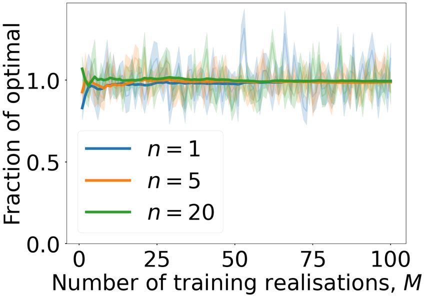
Figure 2: Robustness experiments for NPSA. Expected reward is
evaluated on the processes obtained by independently varying λ0 and ther note that we have observed these qualitative features to
µ0 at test time. A y-value of 1 corresponds to the best possible ex- be robust to variation of the experimental parameters.
pected reward. The curvature of the plots at x = 100 = 1 shows Data Distribution Shift. In this experiment, jobs arrive
how robust the algorithm is with respect to changes in arrival in- over time horizon T = 2π according to a homogeneous Pois-
tensity (left) and value mean (right), with small curvature indicating son process with fixed intensity λ = 500 and have values
robustness and large curvature showing the opposite.
that are exponentially distributed with mean µ = 200. We
simulate M = 30 realisations of the job arrival process and
the arrival intensity λ(t) of the data-generating process dif- derive critical curves via NPSA. We then compute modifiers
fer between training and test time; and finally iii. applying δj for j ∈ {1, . . . , 20}, where the δj are logarithmically
NPSA to public fraud data and evaluating its effectiveness in spaced in the interval [10−2 , 102 ]. The modifiers δj give rise
detection of the most valuable fraudulent transactions. to λ0j = δj · λ and µ0j = δj · µ. We fix a j ∈ {1, . . . , 20}.
Convergence to Optimality. We require a job value dis- Holding µ (resp. λ) constant, we then generate M 0 = 20 re-
tribution F and arrival intensity λ(t) such that we can derive alisations of the job arrival process with arrival rate λ0j (resp.
the optimal reward exactly. We fit φe and λ
e using M simulated mean job value µ0j ) during which we accept jobs according to
realisations of the job arrival process. The reward observed the thresholds derived by NPSA for µ, λ. The mean and stan-
from using NPSA-derived thresholds on further simulations dard error of the reward over the M 0 realisations is recorded
is then compared to the known optimal reward as M grows. and normalised by the optimal reward for the true data gener-
?
Part of the motivation for the development of NPSA stems ating process at test time, r0 .
from the intractability of exactly solving the system of ODEs The result is shown in Figure 2. Note first that the re-
necessitated by Theorem 1 for the optimal critical curves. ward is very robust to variations in arrival rate. Indeed, us-
This strictly limits the F and λ(t) that we can use for this ing thresholds that have been derived for an arrival process
experiment. Thus, we restrict the job arrival process to be ho- where the rate differs by an order of magnitude (either an in-
mogeneous, that is, λ(t) = λ for all t ∈ [0, T ]. We consider crease or decrease) incurs a relatively small penalty in reward
two job-value distributions, i. exponential, that is, (up to 60%), especially when the jobs at test time arrive more
z z
frequently than during training time. The reward is less ro-
F (z) = 1 − e− µ , φ(z) = µe− µ , bust with respect to variations in the mean of the job value,
wherein a difference by an order of magnitude corresponds to
where µ is the mean job value; and ii. Lomax, that is, ≈ 80% loss of reward when n = 20. Nevertheless, for more
ξ α z+ξ α+1 modest deviations from the true µ value the reward is robust.
F (z) = 1 − (1 + zξ )−α , φ(z) = (α−1)(ξ+z)α ,
Evaluation on Public Fraud Data. We augment the
where α > 0 is the shape parameter and ξ > 0 is the SeqAlloc-NP problem setup in Section 2 with the following.
scale. The exponential distribution is the “simplest” distribu- Each job (transaction) is endowed with a feature x ∈ X and a
tion in the maximum entropy sense for a nonnegative r.v. with true class label y ∈ {0, 1}. The decision-maker has access to
known mean. Lomax-distributed r.v.s are related to exponen- x when a job arrives, but not the true label y. They also have
tial r.v.s by exponentiation and a shift and are heavy-tailed. access to a discriminator, D : X → [0, 1] that represents a
4218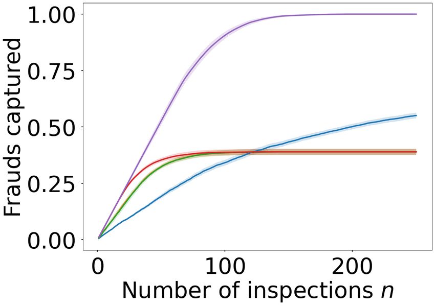
Proceedings of the Thirtieth International Joint Conference on Artificial Intelligence (IJCAI-21)

Dataset       Mtrain Mtest      tot
                               Ndaily     fraud
                                         Ndaily       fraud
                                                     vdaily     clf F1 -score          which we call realised value and ii. how many are truly fraud-
cc-fraud        2      1      94,935      122        17,403        0.9987              ulent, or captured frauds. We compare these quantities ob-
ieee-fraud     114    69     2,853 ± 54 103 ± 4 16,077 ± 738       0.8821
                                                                                       tained from the NPSA algorithm with those obtained from
                                                                                       a number of baselines, in order of increasing capability: i.
Table 1: Dataset properties for Figure 3 experiments. Each dataset
                                                                                       Greedy. Choose the first n transactions clf marks as hav-
has Mtrain realisations of training data and Mtest realisations for test-              ing positive class; ii. Uniform. From all the transactions clf
                    tot
ing. There are Ndaily   transactions per day in the test data, out of                  marks as positive class, choose n transactions uniformly at
          fraud
which Ndaily are fraudulent, with a total monetary value of vdaily  fraud
                                                                          .            random; iii. Hindsight. From all the transactions clf marks
We indicate the F1 -score of the clf classifier on the training set.                   as positive class, choose the n transactions with highest mon-
                                                                                       etary value; iv. Full knowledge. From all the transactions
                                                                                       with y = 1, choose the n transactions with highest mone-
                                                                                       tary value. Note that iv. is included to serve as an absolute
                                                                                       upper-bound on performance. We use two public fraud de-
                                                                                       tection datasets, which we denote cc-fraud [Dal Pozzolo et
                                                                                       al., 2015] and ieee-fraud [IEEE-CIS, 2019]. The relevant
                                                                                       dataset properties are given in Table 1.
                                                                                          The results are shown in Figure 3. First observe that NPSA
                                                                                       shows favourable results even when trained on two realisa-
                                                                                       tions (Mtrain = 2 for the cc-fraud dataset), outperform-
                                                                                       ing even the Hindsight baseline for n ≥ 60 in terms of
                                                                                       captured realised value. On the ieee-fraud dataset with
                                                                                       Mtrain = 114, NPSA is outperformed only by Full Knowledge
                                                                                       after n ≥ 15. In terms of the number of captured frauds, the
                                                                                       intuition that NPSA is waiting to inspect only the most valu-
                                                                                       able transactions to select is validated, evidenced by the the
                                                                                       NPSA curve in these plots lying below the baseline curves,
                                                                                       contrasted with the high realised value.
Figure 3: Fraud detection results for cc-fraud (top) and
ieee-fraud (bottom) datasets. The left plots show the fraction of                      5   Conclusion
daily fraudulent transactions captured and the right show the fraction
of fraudulent monetary value captured.                                                 In this work we introduce the SeqAlloc-NP problem and its
                                                                                       efficient, provably optimal solution via the NPSA algorithm.
                                                                                       Given M independent realisations of a job arrival process,
subjective assessment of probability of a job with side infor-                         we are able to optimally select the n most valuable jobs in
mation x being a member of the positive class, P[y = 1 | x].                           real-time assuming the incoming data follows the same ar-
The adjusted value of a job V (x, v), where v is the job value,                        rival process. This algorithm is robust to variations in the
is given by the expected utility, V (x, v) = D(x)·v, where we                          data-generating process at test-time and has been applied to
stipulate that a job being a member of the positive class yields                       the financial fraud detection problem, when the value of each
utility v, being a member of the negative class yields zero                            transaction is evaluated in a risk-neutral manner.
utility and the decision-maker is risk-neutral. The decision-                             Future work will go down several paths: including investi-
maker now seeks to maximise total expected utility.                                    gating risk-hungry and risk-averse decision-makers; studying
   The reference time frame T is set to one day and the in-                            adversarial job arrival processes; addressing the effect of jobs
dividual realisations are split into Mtest test and Mtrain train-                      taking up a finite time; and specialising to different applica-
ing realisations, ensuring all test realisations occur chrono-                         tion domains.
logically after all training realisations. A classifier clf is                         Disclaimer. This paper was prepared for informational pur-
trained on the transactions in the training set using the F1 -                         poses by the Artificial Intelligence Research group of JPMor-
score as a loss function. This yields the discriminator D( · ) ≡                       gan Chase & Co. and its affiliates (“JP Morgan”), and is not a
clf.predict proba( · ) where clf has a scikit-learn [Pe-                               product of the Research Department of JP Morgan. JP Mor-
dregosa et al., 2011]-type interface. For each transaction with                        gan makes no representation and warranty whatsoever and
side information x and value v, we compute the adjusted                                disclaims all liability, for the completeness, accuracy or re-
value V (x, v). The mean-shortage function φe for the adjusted                         liability of the information contained herein. This document
job value distribution is learned on this data via the scheme                          is not intended as investment research or investment advice,
described in Section 3.3. Given λ(t)
                                   e and φ, e we derive critical                       or a recommendation, offer or solicitation for the purchase or
curves via NPSA for n ∈ {1, . . . , 250}, which are replayed                           sale of any security, financial instrument, financial product or
on the Mtest test realisations. Full details of the clf training                       service, or to be used in any way for evaluating the merits
and data preparation procedure are given in the Supplemen-                             of participating in any transaction, and shall not constitute a
tary Material.                                                                         solicitation under any jurisdiction or to any person, if such
   We are interested in two quantities: i. the total mone-                             solicitation under such jurisdiction or to such person would
tary value of inspected transactions that are truly fraudulent,                        be unlawful.

                                                                                4219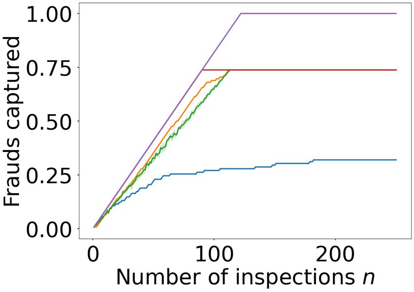
Proceedings of the Thirtieth International Joint Conference on Artificial Intelligence (IJCAI-21)

References                                                                     [IEEE-CIS, 2019] IEEE Computational Intelligence Soci-
[Albright, 1974] C. S. Albright. Optimal sequential assign-                       ety. IEEE-CIS.        IEEE-CIS Fraud Detection, 2019.
   ments with random arrival times. Management Science,                           https://www.kaggle.com/c/ieee-fraud-detection/datasets.
   21(1):60–67, 2020/10/21/ 1974.                                              [Jenatton et al., 2016] R. Jenatton, J. Huang, and C. Archam-
                                                                                  beau. Adaptive algorithms for online convex optimization
[Altman, 1999] E. Altman. Constrained Markov Decision
                                                                                  with long-term constraints. In Proc. ICML, volume 48,
   Processes. Chapman and Hall, 1999.                                             pages 402–411, 2016.
[Avenhaus et al., 1996] R. Avenhaus, M. J. Canty, and                          [Khoshkhou, 2014] G.B. Khoshkhou. Stochastic sequential
   F. Calogero. Compliance Quantified: An Introduction to                         assignment problem. PhD thesis, University of Illinois at
   Data Verification. Cambridge University Press, 1996.                           Urbana-Champaign, 2014.
[Bahnsen et al., 2014] A. C. Bahnsen, D. Aouada, and B. Ot-                    [Law and Kelton, 1991] A. M. Law and D. W. Kelton. Sim-
   tersten. Example-dependent cost-sensitive logistic regres-                     ulation modeling and analysis. McGraw-Hill, 2nd edition,
   sion for credit scoring. In Proc. ICMLA, pages 263–269,                        1991.
   2014.
                                                                               [Mannor and Shimkin, 2004] Shie Mannor and Nahum
[Beyer et al., 2016] B. Beyer, C. Jones, J. Petoff, and N. R.                     Shimkin.       A geometric approach to multi-criterion
   Murphy. Site Reliability Engineering: How Google Runs                          reinforcement learning. JMLR, 5:325–360, 2004.
   Production Systems. O’Reilly Media, Inc., 1st edition,                      [Mannor and Tsitsiklis, 2006] S. Mannor and J. N. Tsitsik-
   2016.
                                                                                  lis. Online learning with constraints. In Learning Theory,
[Bolton and Hand, 2002] R. J. Bolton and D. J. Hand. Sta-                         pages 529–543. Springer Berlin Heidelberg, 2006.
   tistical fraud detection: A review. Statist. Sci., 17(3):235–               [Massart, 1990] P. Massart. The Tight Constant in the
   255, 08 2002.                                                                  Dvoretzky-Kiefer-Wolfowitz Inequality. Ann. Probab.,
[Brauer, 1963] F. Brauer. Bounds for solutions of ordinary                        18(3):1269–1283, 07 1990.
   differential equations. Proc. American Mathematical So-                     [Maxima, 2014] Maxima. Maxima, a Computer Algebra
   ciety, 14(1):36–43, 1963.                                                      System. Version 5.34.1, 2014.
[Consultants, 2019] Cambridge Consultants. Use of AI in                        [Morishita and Okumura, 1983] I. Morishita and M. Oku-
   Content Moderation. Produced on behalf of Ofcom, 2019.                         mura. Automated visual inspection systems for industrial
[Dal Pozzolo et al., 2015] A. Dal Pozzolo, O. Caelen, R. A.                       applications. Measurement, 1(2):59 – 67, 1983.
   Johnson, and G. Bontempi. Calibrating probability with                      [Pedregosa et al., 2011] F. Pedregosa, G. Varoquaux,
   undersampling for unbalanced classification. In 2015                           A. Gramfort, V. Michel, B. Thirion, O. Grisel, M. Blon-
   IEEE Symposium Series on Computational Intelligence,                           del, P. Prettenhofer, R. Weiss, V. Dubourg, J. Vanderplas,
   pages 159–166, 2015.                                                           A. Passos, D. Cournapeau, M. Brucher, M. Perrot, and
[Dal Pozzolo, 2015] A. Dal Pozzolo. Adaptive machine                              E. Duchesnay. Scikit-learn: Machine learning in Python.
   learning for credit card fraud detection. PhD thesis, 2015.                    JMLR, 12:2825–2830, 2011.
[DeGroot, 1970] M. H. DeGroot. Optimal statistical deci-                       [Sakaguchi, 1977] M. Sakaguchi. A sequential allocation
   sions. McGraw-Hill, New York, NY, 1970.                                        game for targets with varying values. Journal of the Oper-
                                                                                  ations Research Society of Japan, 20(3):182–193, 1977.
[Derman et al., 1972] C. Derman, G. J. Lieberman, and
                                                                               [Shen and Kurshan, 2020] H. Shen and E. Kurshan. Deep Q-
   S. M. Ross. A sequential stochastic assignment problem.
                                                                                  Network-based Adaptive Alert Threshold Selection Policy
   Management Science, 18(7):349–355, 1972.
                                                                                  for Payment Fraud Systems in Retail Banking. In Proc.
[Dupuis and Wang, 2002] Paul Dupuis and Hui Wang. Op-                             ICAIF, 2020.
   timal stopping with random intervention times. Advances                     [The Sage Developers, 2020] The Sage Developers. Sage-
   in Applied Probability, 34(1):141–157, 2002.                                   Math, the Sage Mathematics Software System (Version
[Dvoretzky et al., 1956] A. Dvoretzky, J. Kiefer, and J. Wol-                     9.2), 2020.
   fowitz. Asymptotic minimax character of the sample dis-                     [Vaněk et al., 2012] O. Vaněk, Z. Yin, M. Jain, B. Bošanský,
   tribution function and of the classical multinomial estima-                    M. Tambe, and M. Pěchouček. Game-theoretic resource
   tor. Ann. Math. Statist., 27(3):642–669, 09 1956.                              allocation for malicious packet detection in computer net-
[Efroni et al., 2020] Yonathan Efroni, Shie Mannor, and                           works. In Proc. AAMAS, page 905–912, 2012.
   Matteo Pirotta. Exploration-exploitation in constrained                     [Zhao et al., 2020] Peng Zhao, Guanghui Wang, Lijun
   mdps. CoRR, abs/2003.02189, 2020.                                              Zhang, and Zhi-Hua Zhou. Bandit convex optimization in
[Elkan, 2001] C. Elkan. The foundations of cost-sensitive                         non-stationary environments. In Proc. AISTATS, volume
   learning. In Proc. IJCAI, page 973–978, 2001.                                  108, pages 1508–1518, 2020.
[Henderson, 2003] S. G. Henderson. Estimation for nonho-                       [Zheng and Ratliff, 2020] Liyuan Zheng and Lillian J.
   mogeneous poisson processes from aggregated data. Op-                          Ratliff. Constrained upper confidence reinforcement learn-
   erations Research Letters, 31(5):375 – 382, 2003.                              ing. CoRR, abs/2001.09377, 2020.

                                                                        4220
You can also read