NGFS Climate Scenarios Database - Technical Documentation V2.2

NGFS
Climate Scenarios Database

 Technical Documentation V2.2

 JUNE 2021

This document was prepared by:

Christoph Bertram1, Jérôme Hilaire1, Elmar Kriegler1, Thessa Beck2, David N. Bresch3,4, Leon Clarke5, Ryna Cui5,
Jae Edmonds5,6, Molly Charles6, Alicia Zhao5, Chahan Kropf3,Inga Sauer1, Quentin Lejeune2, Peter Pfleiderer2,
Jihoon Min7, Franziska Piontek1, Joeri Rogelj7, Carl-Friedrich Schleussner2, Fabio Sferra7, Bas van Ruijven7, Sha
Yu5,6, Dawn Holland8, Iana Liadze8, and Ian Hurst8

1 Potsdam Institute for Climate Impact Research (PIK), member of the Leibnitz Association, Potsdam, Germany
2 Climate Analytics, Berlin, Germany
3 Institute for Environmental Decisions, ETH Zurich, Zurich, Switzerland
4 Federal Office of Meteorology and Climatology MeteoSwiss, Operation Center 1, Zurich-Airport, Switzerland
5 Center for Global Sustainability, School of Public Policy, University of Maryland, College Park, Maryland, United States of
America
6 Pacific-Northwest National Laboratory (PNNL), United States of America
7 International Institute of Applied System Analysis (IIASA), Laxenburg, Austria
8 National Institute for Economic and Social Research (NIESR), London, United Kingdom

This document was prepared under the auspice of the NGFS WS2 Macrofinancial workstream.

Cite as: Bertram C., Hilaire J, Kriegler E, Beck T, Bresch D, Clarke L, Cui R, Edmonds J, Charles M, Zhao A, Kropf
C, Sauer I, Lejeune Q, Pfleiderer P, Min J, Piontek F, Rogelj J, Schleussner CF, Sferra, F, van Ruijven B, Yu S,
Holland D, Liadze I, Hurst I (2021) : NGFS Climate Scenario Database: Technical Documentation V2.2

Contents

Acknowledgements 2
1. Introduction 3
2. Key technical features of the NGFS Scenarios 4
3. NGFS Scenario Explorer 6
 3.1. Transition pathways for the NGFS scenarios 6
 3.2. Economic impact estimates from physical risks 28
 3.3. Short-term macro-economic effects (NiGEM): 32
 3.4. User manual for the NGFS Scenario Explorer 40

4. Climate Impact Explorer and data 47
 4.1. Introduction to the Climate Impact Explorer 47
 4.2. Methodology behind the Climate Impact Explorer 47
 4.3. Models, scenarios and data sources 55
 4.4. Visualisation 63

Glossary 66
Appendix 75
Bibliography 80

Acknowledgements
The NGFS Scenarios were produced by NGFS Workstream 2 in partnership with an academic consortium from
the Potsdam Institute for Climate Impact Research (PIK), International Institute for Applied Systems Analysis
(IIASA), University of Maryland (UMD), Climate Analytics (CA), Swiss Federal Institute of Technology in Zurich
(ETHZ), and National Institute of Economic and Social Research (NIESR). This work was made possible by
grants from Bloomberg Philanthropies and ClimateWorks Foundation.

Special thanks is given to lead coordinating authors: Christoph Bertram (PIK), Jérôme Hilaire (PIK), Elmar
Kriegler (PIK), contributing authors: Thessa Beck (CA), David N. Bresch (ETHZ), Leon Clarke (UMD), Ryna Yiyun
Cui (UMD), Jae Edmonds (UMD), Molly Charles (PNNL), Alicia Zhao (UMD), Chahan Kropf (ETHZ), Inga Sauer
(PIK), Quentin Lejeune (CA), Peter Pfleiderer (CA), Jihoon Min (IIASA), Franziska Piontek (PIK), Carl-Friedrich
Schleussner (CA), Fabio Sferra (IIASA), Joeri Rogelj (IIASA), Bas van Ruijven (IIASA), Sha Yu (UMD), Dawn
Holland (NIESR), Iana Liadze (NIESR), and Ian Hurst (NIESR) and reviewers: Ryan Barrett (Bank of England),
Antoine Boirard (Banque de France), Clément Payerols (Banque de France) and Edo Schets (Bank of England).

 2

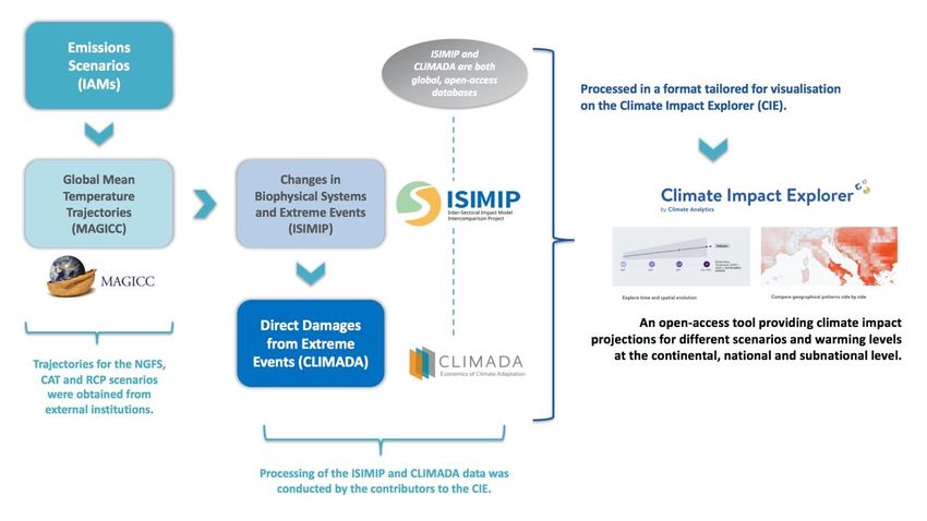
1. Introduction
This document provides technical information on the two datasets behind the NGFS scenarios. It is intended to
answer technical questions for those who want to perform analyses on the datasets themselves. It is an update
of the Technical Documentation published in June 2020 alongside the first set of NGFS Scenarios. It is therefore
aligned with the second set of NGFS Scenarios, released in June 2021.

The two datasets broadly separate transition and physical risk data (see NGFS Climate Scenarios Phase II
Presentation, June 2021 and the NGFS Scenario Portal, June 2021).

  The dataset on transition risk comprises transition pathways, including downscaled information on
 national energy use and emissions and data on macro-economic impacts from physical risks. This
 dataset also contains scenarios of the economic implications of the combined transition and physical
 effects on major economies. These data are available in the NGFS Scenario Explorer provided by
 IIASA (https://data.ene.iiasa.ac.at/ngfs/#/login?redirect=%2Fworkspaces).

  The other dataset covers the physical impact data collected by the Inter-Sectoral Impact Model
 Intercomparison Project (ISIMIP), as well as data from CLIMADA, both of which are accessible via the
 NGFS Climate Impact Explorer provided by CA (http://climate-impact-
 explorer.climateanalytics.org/). These datasets are generated with a suite of models including
 integrated assessment models, a macro-econometric model, earth system models, sectoral impact
 models, a natural catastrophe damage model and global macroeconomic damage functions. They are
 linked together in a coherent way by aligning global warming levels and by explicit linkage via defined
 interfaces in case of the integrated assessment models and the macro-econometric model. For each
 dataset, the most important technical details of the underlying academic work and a short user guide
 are provided here. These are complemented by links to other resources with more detailed
 information.

This document is intended to answer technical questions for those who want to perform analyses on the
datasets themselves, but does not address conceptual questions. For a high-level description of the NGFS
scenarios and the rationale behind them, please consult the NGFS Scenario Portal including an FAQ section and
the NGFS Climate Scenarios Phase II Presentation For a broad overview on how to perform scenario analysis in
a financial context, please refer to the NGFS Guide to climate scenario analysis for central banks and supervisors.
This document reflects the status of existing scenarios and datasets that are used in the current NGFS
presentation and documents.

Please note that this is the follow-up product which supersedes the first publication from 2020. Key novelties
relate to the bespoke narratives of the transition scenarios, a downscaling of key results to country level, the
linkage to the macro-econometric model NiGEM, and the inclusion of CLIMADA data and the set-up of the CIE,
as well as the NGFS scenario portal.

This document is structured as follows: Section 2 presents the main technical features of the NGFS scenarios.
Section 3 introduces the NGFS Scenario Explorer dataset, including technical details and assumptions for the
modelling of the transition pathways, and details about how the outputs from this modelling are used to
calculate ex-post macro-economic damage estimates from physical risks based on different macro
methodologies. Section 4 introduces ISIMIP climate impact data which are relevant for assessing physical risks,
including details on model and scenario assumptions and information on variables available in the datasets and
their definitions.

User manuals for each of the two datasets are provided at end of their respective sections (see sections 3.4 and
4.4).

 3

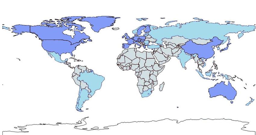
2. Key technical features of the NGFS Scenarios
The NGFS reference scenarios consist of 6 scenarios which cover three of the four quadrants of the NGFS
scenario matrix (i.e. orderly, disorderly and hot house world) (see Figure 1). From a transition risk perspective,
these 6 scenarios were considered by three contributing modelling groups (IIASA, PIK and UMD 1), yielding a
total of 18 transition pathways (i.e. across different scenarios and models).

Figure 1 Overview of the NGFS scenarios. Scenarios are indicated with bubbles and positioned according to
their transition and physical risks.

The range of scenarios and models allows users to explore uncertainties both by comparing different scenarios
from a single model and by comparing the ranges from the three models for a given scenario (for further details
on model characteristics and differences see section 3.1.1).

The transition pathways all share the same underlying assumption on key socio-economic drivers, such as
harmonised population and economic developments. Further drivers such as food and energy demand are also
harmonised, though not at a precise level but in terms of general patterns. All these socio-economic
assumptions are taken from the shared socio-economic pathway SSP2 (Dellink et al., 2017; Fricko et al., 2017;
KC & Lutz, 2017; O’Neill et al., 2017; Riahi, van Vuuren, et al., 2017), which describes a “middle-of-the-road”
future. In order to account for the COVID-19 pandemic and its impact on economic systems and growth, the
GDP and final energy demand trajectories have been adjusted based on projections from the IMF (IMF 2020).
Many of these input and quasi-input assumptions are reported in the database, see section 3.1.3 for details.

Scenarios are differentiated by three key design choices relating to long-term policy, short-term policy, and
technology availability, see section 3.1.2 for details. Scenario names reflect these choices and have been
harmonised across models.

1
 See glossary for a description of these modelling groups

 4

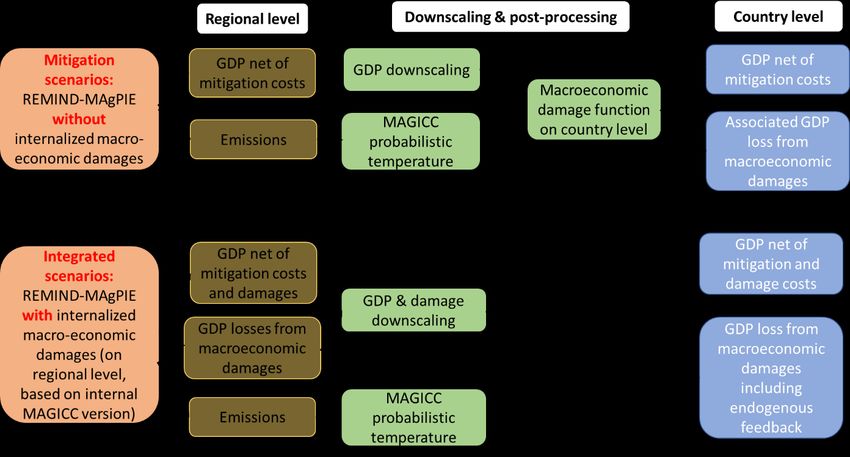
The transition pathways do not incorporate economic damages from physical risks by default, so economic
trajectories are projected without consideration of feedbacks from emissions and temperature change onto
infrastructure systems and the economy. As a step towards more integrated analysis, three approaches for
incorporating the physical risk side are possible with the reference scenario set.

Approach 1: Macro-economic damage function

Section 3.2 details how estimates of potential macro-economic damages from physical risk can be computed
using simple damage functions, using the temperature outcomes inferred from the emissions trajectories
projected by the transition scenarios. This approach has been integrated in the macro-economic modelling of
the NGFS scenarios.

Approach 2: Integrated

As described in section 3.2.3, one of the models (REMIND-MAgPIE) additionally ran a subset of scenarios with
an implementation of internalized physical risk damages.

Approach 3: Sector-level impact data

Section 4 offers sector-level impact data, based on various sector models, available for two separate
temperature projections. These temperature projections are based on earlier harmonized scenarios but are
broadly similar (though not identical) to the transition pathways above. They can be mapped to the NGFS
scenarios in the following way: the orderly and disorderly 1.5°C and 2°C scenarios are in the range of the low
temperature scenario (Representative Concentration Pathway RCP2.6), whereas the Current policies scenario
is close to the high temperature scenario (RCP 6.0) by the end of the century.

 5

3. NGFS Scenario Explorer

3.1. Transition pathways for the NGFS scenarios

3.1.1. Contributing integrated assessment models
The transition pathways for the NGFS scenarios have been generated with three well-established integrated
assessment models (IAMs), namely GCAM, MESSAGEix-GLOBIOM and REMIND-MAgPIE. These models have
been used in hundreds of peer-reviewed scientific studies on climate change mitigation. In particular, they allow
the estimation of global and regional mitigation costs (Kriegler et al., 2013, 2014, 2015; Luderer et al., 2013;
Riahi et al., 2015; Tavoni et al., 2013), the analysis of emissions pathways (Riahi, van Vuuren, et al., 2017; Rogelj,
Popp, et al., 2018), associated land use (Popp et al., 2017) and energy system transition characteristics (Bauer
et al., 2017; GEA, 2012; Kriegler et al., 2014; McJeon et al., 2014), the quantification of investments required to
transform the energy system (GEA, 2012; McCollum et al., 2018; Bertram et al., 2021) and the identification of
synergies and trade-offs of sustainable development pathways (Bertram et al., 2018; TWI2050, 2018).
Importantly, their results feature in several assessment reports (Clarke et al., 2014; Forster et al., 2018; Jia et
al., In press; Rogelj, Shindell, et al., 2018; UNEP, 2018). Consequently, these models have a long tradition of
catering key climate change mitigation information to policy and decision makers. MESSAGEix-GLOBIOM and
REMIND-MAgPIE were also recently used to evaluate the transition risks faced by banks (UNEP-FI, 2018).

The three models share a similar structure. They combine macro-economic, agriculture and land-use, energy,
water and climate systems into a common numerical framework that enables the analysis of the complex and
non-linear dynamics in and between these components. In contrast to smaller IAMs like DICE and RICE, the
IAMs used here cover more systems with a finer granularity and process detail. For instance, they offer more
detailed representations of the energy system that include many technologies and account for capacity
vintages and technological change. This in turn allows the generation of more detailed transition pathways.

In addition, GCAM, MESSAGEix-GLOBIOM and REMIND-MAgPIE generate cost-effective transition pathways.
That is, they provide pathways that minimise costs subject to a range of constraints that can vary with scenario
design like limiting warming to below 2°C and techno-economic and policy assumptions. It is worthwhile to
note that these models in general do not account for climate damages (the additional exploratory scenarios
with REMIND-MAgPIE are the exception, see section 3.2.3) and so cannot be used for cost-benefit analysis or
to compute the social cost of carbon.

The models feature many climate change mitigation options including energy-demand-side, energy-supply-
side, Agriculture, Forestry and Other Land Uses (AFOLU) and carbon dioxide removal (CDR) measures (see
Table 1). The energy sector is expected to play a huge role in the transition to a low-carbon economy as it
currently accounts for the highest share of emissions and offers the greatest number of mitigation options.
These include solar, wind, nuclear power, carbon capture and storage (CCS), fuel cells and hydrogen on the
supply side and energy efficiency improvements, electrification and CCS on the demand side. There are also
several mitigation options in the AFOLU sectors, such as reduced deforestation/forest protection/avoided
forest conversion, forest management, methane reductions in rice paddies, or nitrogen pollution reductions.
Finally, all models include at least two CDR technologies, namely bioenergy with carbon capture and storage
(BECCS) as well as afforestation and reforestation.

 6

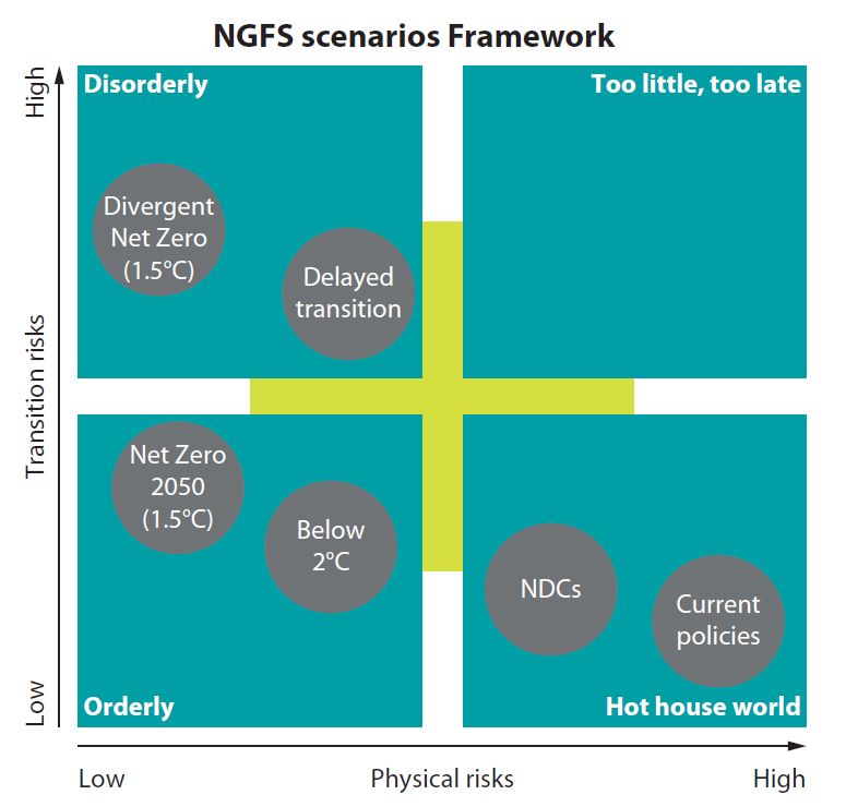
Table 1 Overview of mitigation options in GCAM, MESSAGEix-GLOBIOM and REMIND-MAgPIE (adapted
from Rogelj et al. (2018) and table 2.SM.6 in Forster et al. (2018))
 GCAM MESSAGEix-GLOBIOM REMIND-MAgPIE

# Demand side
 14 16 15
mitigation options

Examples of Energy efficiency Energy efficiency Energy efficiency
demand side improvements, improvements, improvements,
measures electrification of buildings, electrification of buildings, electrification of buildings,
 industry and transport industry and transport industry and transport
 sectors, CCS in industrial sectors, CCS in industrial sectors, CCS in industrial
 process applications process applications process applications

# Supply side
 18 20 17
mitigation options

Examples of supply Solar PV, Wind, Nuclear, Solar PV, Wind, Nuclear, Solar PV, Wind, Nuclear,
side measures CCS, Hydrogen CCS, Hydrogen CCS, Hydrogen

# AFOLU options 8 8 7

Examples of AFOLU Reduced Reduced Reduced
measures deforestation/forest deforestation/forest deforestation/forest
 protection/avoided forest protection/avoided forest protection/avoided forest
 conversion, Forest conversion, Forest conversion, Methane
 management, Methane management, reductions in rice paddies,
 reductions in rice paddies, Conservation agriculture, Nitrogen pollution
 Nitrogen pollution Methane reductions in rice reductions
 reductions paddies, Nitrogen pollution
 reductions

Although the models share similarities, each has its own characteristics (see Table 1 and Table 2) which can
influence results (i.e. model fingerprints). For instance, from an economic perspective, both MESSAGEix-
GLOBIOM and REMIND-MAgPIE are general equilibrium models solved with an intertemporal optimisation
algorithm (i.e. perfect foresight). This allows the models to fully anticipate changes occurring over the 21 st
century (e.g. increasing costs of exhaustible resources, declining costs of solar and wind technologies,
increasing carbon prices) and also allows for an endogeneous change in consumption, GDP and demand for
energy in response to climate policies.

In contrast, GCAM is a partial equilibrium model of the land use and energy sectors and consequently, takes
exogenous assumptions on GDP development and energy demands. It features also a “myopic” view of the
future. At each time step agents in GCAM consider only past and present circumstances in formulating their
behaviour including expectations for the future. Prior information includes such factors as existing capital
stocks. Expectations for the future are that then current prices and policies will persist for the life of the capital
investment. This difference in modelling approach can affect investment dynamics in technologies, e.g. the
deployment of carbon dioxide removal technologies.

 7

Table 2 Overview of key model characteristics (see also reference cards 2.6, 2.15, and 2.17 in Forster et al.
(2018))
 Integrated Assessment GCAM 5.3 MESSAGEix_GLOBIOM 1.1 REMIND-MAgPIE 2.1-4.2
 Model

Short name GCAM MESSAGEix-GLOBIOM REMIND-MAgPIE

Solution concept Partial Equilibrium (price General Equilibrium (closed REMIND: General
 elastic demand) economy) Equilibrium (closed
 economy)

 MAgPIE: Partial Equilibrium
 model of the agriculture
 sector

Anticipation Recursive dynamic Intertemporal (perfect REMIND: Inter-temporal
 (myopic) foresight) (perfect foresight)

 MAgPIE: recursive dynamic
 (myopic)

Solution method Cost minimisation Welfare maximisation REMIND: Welfare
 maximisation

 MAgPIE: Cost minimisation

Temporal dimension Base year: 2015 Base year: 1990 Base year: 2005

 Time steps: 5 years Time steps: 5 (2005-2060) Time steps: 5 (2005-2060)
 and 10 years (2060-2100) and 10 years (2060-2100)
 Horizon: 2100
 Horizon: 2100 Horizon: 2100

Spatial dimension 32 world regions 11 world regions 12 world regions

Technological Exogenous Exogenous Endogenous for Solar, Wind
change and Batteries

Technology 58 conversion technologies 64 conversion technologies 50 conversion technologies
dimension

Demand sectors and Buildings, Industry Buildings, Industry, Buildings, Industry (Cement,
subsector detail (Cement, Chemicals, Steel, Transport Chemicals, Steel, Other),
 Non-ferrous metals, Transport
 Other), Transport

Modelling teams strive for a high level of transparency. The models are well documented across several peer-
reviewed publications, IPCC assessment reports (e.g. reference cards 2.6, 2.15, and 2.17 in Forster et al. (2018)),
publicly-available technical documentations and wikis (e.g. www.iamcdocumentation.eu). At the time of
writing this document, the GCAM and MAgPIE models are fully open-source. The source code of the
MESSAGEix-GLOBIOM and REMIND models are available in open access and the modelling teams are currently
working on making them fully open-source. The links to these models and their documentation are given in the
following sections, which provide a more detailed account of the three IAMs.

A comprehensive primer on climate scenarios is available in the SENSES toolkit
(https://climatescenarios.org/primer/primer). This web platform also offers learn modules to enhance

 8

understanding on a number of topics such as future electrification, fossil fuels risks and closing the emissions
gap.

GCAM

GCAM is a global model that represents the behavior of, and interactions between five systems: the energy
system, water, agriculture and land use, the economy, and the climate (Figure 2). GCAM has been under
development for 40 years. Work began in 1980 with the work first documented in 1982 in working papers and
the first peer-reviewed publications in 1983 (J. Edmonds & Reilly, 1983a, 1983b, 1983c). At this point, the model
was known as the Edmonds-Reilly (and subsequently the Edmonds-Reilly-Barnes) model. The current version
of the model is documented at https://jgcri.github.io/gcam-doc/overview.html and at Calvin et al. (Calvin et al.,
2019).

GCAM includes two major computational components: a data system to develop inputs and the GCAM core.
The GCAM Data System combines and reconciles a wide range of different data sets and systematically
incorporates a range of future assumptions. The output of the data system is an XML dataset with historical
and base-year data for calibrating the model along with assumptions about future trajectories such as GDP,
population, and technology. The GCAM core is the component in which economic decisions are made (e.g.,
land use and technology choices), and in which dynamics and interactions are modeled within and among
different human and Earth systems. The GCAM core is written in C++ and takes in inputs in XML. Outputs are
written to a XML database.

GCAM takes in a set of assumptions and then processes those assumptions to create a full scenario of prices,
energy and other transformations, and commodity and other flows across regions and into the future. The
interactions between these different systems all take place within the GCAM core; that is, they are not modeled
as independent modules, but as one integrated whole.

The exact structure of the model is data driven. In all cases, GCAM represents the entire world, but it is
constructed with different levels of spatial resolution for each of these different systems. In the version of
GCAM used for this study, the energy-economy system operates at 32 regions globally, land is divided into 384
subregions, and water is tracked for 235 basins worldwide. The Earth system module operates at a global scale
using Hector, a physical Earth system emulator that provides information about the composition of the
atmosphere based on emissions provided by the other modules, ocean acidity, and climate.

The core operating principle for GCAM is that of market equilibrium. Representative agents in GCAM use
information on prices, as well as other information that might be relevant, and make decisions about the
allocation of resources. These representative agents exist throughout the model, representing, for example,
regional electricity sectors, regional refining sectors, regional energy demand sectors, and land users who have
to allocate land among competing crops within any given land region. Markets are the means by which these
representative agents interact with one another. Agents indicate their intended supply and/or demand for
goods and services in the markets. GCAM solves for a set of market prices so that supplies and demands are
balanced in all these markets across the model. The GCAM solution process is the process of iterating on market
prices until this equilibrium is reached. Markets exist for physical flows such as electricity or agricultural
commodities, but they also can exist for other types of goods and services, for example tradable carbon
permits.

 9

Figure 2 Schematic representation of the GCAM model.

While the agents in the GCAM model are assumed to act to maximise their own self-interest, the model as a
whole is not performing an optimisation calculation. Decision-making throughout GCAM uses a logit
formulation (J. F. Clarke & Edmonds, 1993; McFadden, 1973). In such a formulation, options are ordered based
on preference, with either cost (as in the energy system) or profit (as in the land system) determining the order.
Given the logit formulation, the single best choice does not capture the entire market, only the largest fraction,
while more expensive/less profitable options also gain some market share, accounting for not explicitly
represented user and technology heterogeneity.

GCAM is a dynamic recursive model, meaning that decision-makers do not know the future when making a
decision. (In contrast, intertemporal optimisation models like MESSAGEix-GLOBIOM and REMIND-MAgPIE
assume that agents know the entire future with certainty when they make decisions). After it solves each
period, the model then uses the resulting state of the world, including the consequences of decisions made in
that period - such as resource depletion, capital stock retirements and installations, and changes to the
landscape - and then moves to the next time step and performs the same exercise. For long-lived investments,
decision-makers may account for future profit streams, but those estimates would be based on current prices.
GCAM is typically operated in five-year time steps with 2015 as the final calibration year. However, the model
has flexibility to be operated at different temporal resolutions through user-defined parameters.

A reference card description of this model can be found as section 2.SM.2.5 in (Forster et al., 2018).

A comprehensive documentation of the model is available at this URL: https://jgcri.github.io/gcam-
doc/overview.html

The source code of the model is open-source and available at this URL: https://github.com/JGCRI/gcam-core

 10

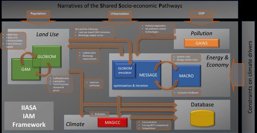
MESSAGEix-GLOBIOM

MESSAGEix-GLOBIOM is a shorthand used to refer to the IIASA IAM framework, which consists of a
combination of five different models or modules - the energy model MESSAGE, the land use model GLOBIOM,
the air pollution and greenhouse gas model GAINS, the aggregated macro-economic model MACRO and the
simple climate model MAGICC - which complement each other and are specialised in different areas. All models
and modules together build the IIASA IAM framework, referred to as MESSAGE-GLOBIOM historically owing
to the fact that the energy model MESSAGE and the land use model GLOBIOM are its central components. The
five models provide input to and iterate between each other during a typical scenario development cycle. Below
is a brief overview of how the models interact with each other.

Recently, the scientific software structure underlying the global MESSAGE-GLOBIOM model was revamped
and called the MESSAGEix framework (Huppmann et al., 2019), an open-source, versatile implementation of a
linear optimisation problem, with the option of coupling to the computable general equilibrium (CGE) model
MACRO to incorporate the effect of price changes on economic activity and demand for commodities and
resources. The new framework is integrated with the ix modeling platform (ixmp), a “data warehouse” for
version control of reference timeseries, input data and model results. ixmp provides interfaces to the scientific
programming languages Python and R for efficient, scripted workflows for data processing and visualisation of
results. The IIASA IAM fleet based on this newer framework is named as MESSAGEix-GLOBIOM.

The name “MESSAGE" itself refers to the core of the IIASA IAM framework (Figure 3) and its main task is to
optimise the energy system so that it can satisfy specified energy demands at the lowest costs (Huppmann
et al., 2019). MESSAGE carries out this optimisation in an iterative setup with MACRO, a single sector macro-
economic model, which provides estimates of the macro-economic demand response that results from energy
system and services costs computed by MESSAGE. The models run on a 11-region global disaggregation. For
the six commercial end-use demand categories depicted in MESSAGE, based on demand prices MACRO will
adjust useful energy demands, until the two models have reached equilibrium. This iteration reflects price-
induced energy efficiency adjustments that can occur when energy prices change.

GLOBIOM provides MESSAGE with information on land use and its implications, including the availability and
cost of bioenergy, and availability and cost of emission mitigation in the AFOLU (Agriculture, Forestry and
Other Land Use) sector. To reduce computational costs, MESSAGE iteratively queries a GLOBIOM emulator
which provides an approximation of land-use outcomes during the optimisation process instead of requiring
the GLOBIOM model to be rerun iteratively. Only once the iteration between MESSAGE and MACRO has
converged, the resulting bioenergy demands along with corresponding carbon prices are used for a concluding
analysis with the full-fledged GLOBIOM model. This ensures full consistency of the results from MESSAGE and
GLOBIOM, and also allows producing a more extensive set of land-use related indicators, including spatially
explicit information on land use.

Air pollution implications of the energy system are accounted for in MESSAGE by applying technology-specific
air pollution coefficients derived from the GAINS model. This approach has been applied to the SSP process
(Rao et al., 2017). Alternatively, GAINS can be run ex-post based on MESSAGEix-GLOBIOM scenarios to
estimate air pollution emissions, concentrations and the related health impacts. This approach allows analysing
different air pollution policy packages (e.g., current legislation, maximum feasible reduction), including the
estimation of costs for air pollution control measures. Examples for applying this way of linking MESSAGEix-
GLOBIOM and GAINS can be found in (McCollum et al., 2018) and (Grubler et al., 2018).

In general, cumulative global carbon emissions from all sectors are constrained at different levels, with
equivalent pricing applied to other greenhouse gases, to reach the desired radiative forcing levels (see right-
hand side in Figure 3). The climate constraints are thus taken up in the coupled MESSAGE-GLOBIOM

 11

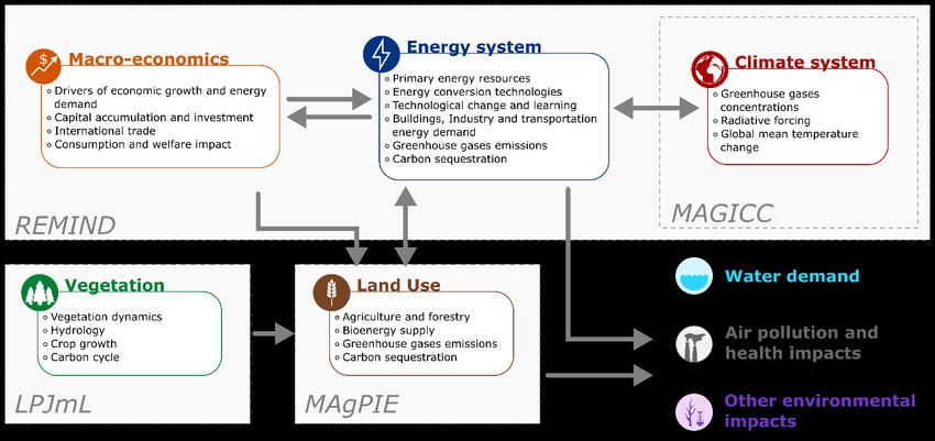
optimisation, and the resulting carbon price is fed back to the full-fledged GLOBIOM model for full consistency.
Finally, the combined results for land use, energy, and industrial emissions from MESSAGE and GLOBIOM are
merged and fed into MAGICC, a global carbon-cycle and climate model, which then provides estimates of the
climate implications in terms of atmospheric concentrations, radiative forcing, and global-mean temperature
increase. Importantly, climate impacts, and impacts of the carbon cycle are thus not accounted for in the IIASA
IAM framework version used for the NGFS scenarios. This is also shown in Figure 3, where the information flow
through the climate model is not fed back into the IAM components.

The entire framework is linked to an online database infrastructure which allows straightforward visualisation,
analysis, comparison and dissemination of results (Riahi, van Vuuren, et al., 2017).

Figure 3 Overview of the IIASA IAM framework, a.k.a. MESSAGEix-GLOBIOM model. Coloured boxes
represent respective specialised disciplinary models which are integrated for generating internally consistent
scenarios (Fricko et al., 2017).

A reference card description of this model can be found as section 2.SM.2.15 in (Forster et al., 2018).

A comprehensive documentation of the model is available at this URLs: https://docs.messageix.org/en/stable/
; https://www.iamcdocumentation.eu/index.php/Model_Documentation_-_MESSAGE-GLOBIOM

The source code of the model is open-source and available at this URL: https://github.com/iiasa/message_ix

REMIND-MAgPIE

REMIND-MAgPIE is a comprehensive IAM framework that simulates, in a forward-looking fashion, the
dynamics within and between the energy, land-use, water, air pollution and health, economy and climate
systems. The models were created over a decade ago (Leimbach, Bauer, Baumstark, & Edenhofer, 2010; Lotze-
Campen et al., 2008) and are continually being improved to provide up-to-date scientific evidence to decision
and policy makers and other relevant stakeholders on climate change mitigation and Sustainable Development
Goals strategies.

The REMIND-MAgPIE framework consists of four main components (see Figure 4). First the REMIND model
combines a macro-economic module with an energy system module. The macro-economic core of REMIND is

 12

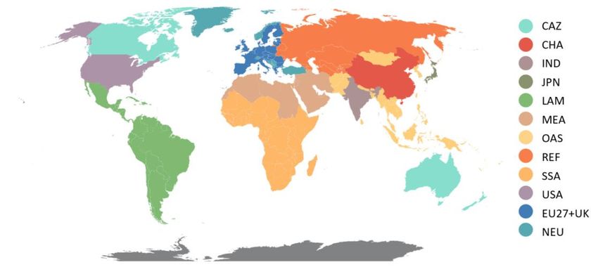
a Ramsey-type optimal growth model in which inter-temporal welfare is maximised. The energy system
module includes a detailed representation of energy supply and demand sectors. Second the MAgPIE model
represents land-use dynamics. The MAgPIE model is linked to the dynamic global vegetation model LPJmL
(Bondeau et al., 2007; Müller & Robertson, 2014; Schaphoff et al., 2017). For some applications that do not
require detailed land-use information, a MAgPIE-based emulator is used to make the scenario generation
process more efficient. The REMIND model is linked to the climate model MAGICC to account for changes in
climate-related variables like global surface mean temperature. In addition, REMIND can be linked to other
models to allow the analysis of other environmental impacts such as water demand, air pollution and health
effects.

Figure 4 Overview of the structure of the REMIND-MAgPIE framework

Specifically, REMIND (Regional Model of Investment and Development) is an energy-economy general
equilibrium model linking a macro-economic growth model with a bottom-up engineering-based energy
system model. It covers 12 world regions (see Figure 5 and Table A1.3 in Appendix 1), differentiates various
energy carriers and technologies and represents the dynamics of economic growth and international trade
(Leimbach, Bauer, Baumstark, & Edenhofer, 2010; Leimbach, Bauer, Baumstark, Luken, et al., 2010; Leimbach
et al., 2017; Mouratiadou et al., 2016). A Ramsey-type growth model with perfect foresight serves as a macro-
economic core projecting growth, savings and investments, factor incomes, energy and material demand. The
energy system representation differentiates between a variety of fossil, biogenic, nuclear and renewable
energy resources (Bauer et al., 2017; Bauer et al., 2012; Bauer et al., 2016; Klein et al., 2014, 2014; Pietzcker et
al., 2014). The model accounts for crucial drivers of energy system inertia and path dependencies by
representing full capacity vintage structure, technological learning of emergent new technologies, as well as
adjustment costs for rapidly expanding technologies (Pietzcker et al., 2017). The emissions of greenhouse gases
and air pollutants are largely represented by source and linked to activities in the energy-economic system
(Strefler, Luderer, Aboumahboub, et al., 2014; Strefler, Luderer, Kriegler, et al., 2014). Several energy sector
policies are represented explicitly (Bertram et al., 2015, 2018; Kriegler et al., 2018), including energy-sector fuel
taxes and consumer subsidies (Jewell et al., 2018; Schwanitz et al., 2014). The model also represents trade in
energy resources (Bauer et al., 2015).

 13

Figure 5 Regional definitions used in the REMIND model

MAgPIE (Model of Agricultural Production and its Impacts on the Environment) is a global multi-region
economic land-use optimization model designed for scenario analysis up to the year 2100. It is a partial
equilibrium model of the agricultural sector that is solved in recursive dynamic mode. The objective function of
MAgPIE is the fulfilment of agricultural demand for 10 world regions at minimum global costs under
consideration of biophysical and socio-economic constraints. Major cost types in MAgPIE are factor
requirement costs (capital, labour, fertiliser), land conversion costs, transportation costs to the closest market,
investment costs for yield-increasing technological change (TC) and costs for greenhouse gas emissions in
mitigation scenarios. Biophysical inputs (0.5° resolution) for MAgPIE, such as agricultural yields, carbon
densities and water availability, are derived from a dynamic global vegetation, hydrology and crop growth
model, the Lund-Potsdam-Jena model for managed Land (LPJmL) (Bondeau et al., 2007; Müller & Robertson,
2014; Schaphoff et al., 2017). Agricultural demand includes demand for food (Bodirsky & Popp, 2015), feed
(Weindl et al., 2015), bioenergy (Humpenöder et al., 2018; Popp et al., 2010), material and seed. For meeting
the demand, MAgPIE endogenously decides, based on cost-effectiveness, about intensification of agricultural
production, cropland expansion and production relocation (intra-regionally and inter-regionally through
international trade) (Dietrich et al., 2014; Lotze-Campen et al., 2010; Schmitz et al., 2012). MAgPIE derives cell
specific land-use patterns, rates of future agricultural yield increases(Dietrich et al., 2014), food commodity and
bioenergy prices as well as GHG emissions from agricultural production (Bodirsky et al., 2012; Popp et al., 2010)
and land-use change (Humpenöder et al., 2014; Popp et al., 2014, 2017).

The coupling approach between REMIND and MAgPIE is designed to derive scenarios with equilibrated
bioenergy and emissions markets. In equilibrium, bio-energy demand patterns computed by REMIND are
fulfilled in MAgPIE at the same bioenergy and emissions prices that the demand patterns were based on.
Moreover, the emissions in REMIND emerging from pre-defined climate policy assumptions account for the
greenhouse gas emissions from the land-use sector derived in MAgPIE under the emissions pricing and
bioenergy use mandated by the same climate policy. The simultaneous equilibrium of bioenergy and emissions
markets is established by an iteration of REMIND and MAgPIE simulations in which REMIND provides emissions
prices and bioenergy demand to MAgPIE and receives land use emissions and bioenergy prices from MAgPIE
in return. The coupling approach with this iterative process at its core is explained elsewhere (Bauer et al., 2014).

MAGICC (Model for the Assessment of Greenhouse-gas Induced Climate Change) is a reduced-complexity
climate model that calculates atmospheric concentrations of greenhouse gases and other atmospheric climate
drivers, radiative forcing and global annual-mean surface air temperature. Emission pathways computed by
REMIND are fed to MAGICC to estimate future changes in climate-related variables.

 14

The REMIND-MAgPIE version with integrated damages is described in section 3.2.3.

A reference card description of this model can be found as section 2.SM.2.17 in (Forster et al., 2018).

Comprehensive documentations of the models are available at these URLs:
https://www.iamcdocumentation.eu/index.php/Model_Documentation_-_REMIND
https://rse.pik-potsdam.de/doc/magpie/4.0/

The source codes of the models are open-source and available at these URLs:
https://github.com/remindmodel/remind
https://github.com/magpiemodel/magpie

3.1.2. Scenario and model input assumptions

The transition pathways for the NGFS Scenarios are differentiated by a number of key design choices relating
to long-term temperature targets, net-zero targets, short-term policy, overall policy coordination and
technology availability. The different assumptions on these design choices are highlighted in table 3, and the
design choices are each explained in more detail below.

The first design choice relates to assumptions on long-term climate policy ("Climate Ambition" in table 3), and
three fundamentally different assumptions are covered by the set of scenarios:

 1. Current policies: existing climate policies remain in place, but there is no strengthening of ambition
 level of these policies. The detail of policy representation differs across models and even within models
 across different sectors. Policy implementation has been included as detailed as possible, but due to
 limited granularity of sector representation, all models also represent some policies as proxies, for
 example via aggregate final energy reductions instead of explicit implementation of efficiency
 standards, or a carbon price.
 2. Nationally determined contributions (NDCs): This scenario foresees that currently pledged
 unconditional NDCs are implemented fully, and respective targets on energy and emissions in 2025
 and 2030 are reached in all countries. The cut-off date for targets being considered here is December
 2020, so the new targets of the EU and China are being reflected in these scenarios, while the new US
 NDC announced in April 2021 is not yet reflected. Teams have instead assumed an ambition level
 corresponding to the previous US NDC for 2025. The long-term policy assumption beyond current
 NDC target times (2025 and 2030) is that climate policy ambition remains comparable to levels implied
 by NDCs. This extrapolation of policy ambition levels over the period 2030-2100 is however subject to
 large uncertainties and is implemented differently in the three models, so long-term deviations across
 scenarios are quite high.
 3. While the long-term evolution of emissions and thus temperature in the above two scenario narratives
 in the hot-house world quadrant result from an extrapolation of near-term policy ambition, the four
 scenarios in the orderly and disorderly quadrants explicitly impose temperature targets. For the Net
 Zero 2050 and Divergent Net Zero scenarios a 1.5°C temperature target was imposed, such that the
 median temperature is required to return to below 1.5°C in 2100, after a limited temporary overshoot.
 The Below 2°C scenario keeps the 67th-percentile of warming below 2°C throughout the 21st century,
 while the Disorderly ”Delayed transition” scenario only imposes this target in 2100 and allows for
 temporary overshoot.

Regarding net-zero targets, the “Net Zero 2050” scenario foresees global CO2 emissions to be at net-zero in
2050. Furthermore, countries with a clear commitment to a specific net-zero policy target at the end of 2020
(i.e. China, EU, Japan, and USA) are assumed to meet this target. For the rest of world it is the case that in 2050

 15

net negative emissions in some countries offset the positive emissions in other countries. The regional net-zero
targets for countries with clear commitments are also prescribed in the “Disorderly Transition” scenario, but
not imposed for the rest of the world, thus leading to strong regional differentiation of efforts.

Regarding short-term policy (“policy reaction”), two alternative assumptions are explored:

 1. Immediate scenarios assume that optimal carbon prices in line with the long-term targets are
 implemented immediately after the 2020 model time step.
 2. The Disorderly ”Delayed transition” scenario by contrast assumes that the next 10 years see a
 "fossil recovery” and thus follow the trajectory of the current policies scenario until 2030. After 2030,
 these scenarios also foresee implementation of a carbon price trajectory in line with long-term
 targets. Importantly, this sudden shift of policy stringency is not anticipated in the two perfect
 foresight models REMIND-MAgPIE and MESSAGEix-GLOBIOM by fixing the variables until 2030
 onto their values of the current policies scenarios.

Regarding overall policy coordination (“regional policy variation”), the scenarios all feature some form of
regional differentiation owing the policy settings described above, but are representing high policy
coordination across sectors in each country/region. The exception is the “Divergent Net Zero” scenario, in
which the carbon prices for transport and buildings are assumed to be three times the carbon price in the supply
and industry sectors, illustrating the additional risks and costs of lack of coordination.

Regarding technology availability, the literature has explored the sensitivity of results to a range of
technological and socio-technical assumptions regarding renewables (Creutzig et al., 2017; Pietzcker et al.,
2017), end-use efficiency (Grubler et al., 2018), nuclear (Bauer et al., 2012), bioenergy (Bauer et al., 2018),
carbon capture and storage (Koelbl et al., 2014) and various land-use related options (Humpenöder et al., 2018;
Popp et al., 2017). Given that each of the three models represented in the NGFS dataset have chosen particular
structural and parametric assumptions in the representation of these alternative mitigation options, the
comparison of the same scenario narrative within different models allows for an estimation of the order of
magnitude that the uncertainties regarding future potentials entail.

One consistent finding of literature with structured comparison of technological sensitivities (Kriegler et al.,
2014; Luderer et al., 2013; Riahi et al., 2015) is that the assumptions on availability of carbon dioxide removal
(CDR) have a particularly profound impact on mitigation trajectories, as higher availability enables a more
gradual phase-out of the use of liquid fuel across various sectors and end-uses. Therefore, the only
technological differentiation explicitly covered in the NGFS dataset is the assumption on availability of
carbon-dioxide removal, with two alternative assumptions:

  Medium availability of carbon sequestration: The orderly scenarios include the same criteria for
 constraints on CDR options (especially bioenergy with carbon capture and storage (BECCS) and
 afforestation) as for other technologies, like biophysical constraints, technological ramp-up
 constraints, exclusion of unsuitable and protected areas, and geological potentials. Based on evolving
 scientific insights on these constraints, and on limited experience with these options in recent years
 which further constrains the near-term ramp-up, CDR levels are lower than in the first set of NGFS
 scenarios.
  Low availability of carbon sequestration: Given that there are particular challenges associated with
 the deployment of all CDR options (Fuss et al., 2018), especially at larger scale, the disorderly scenarios
 add explicit, more conservative constraints on maximum potential for CDR options and on their
 upscaling. In all three models, this is done via explicit constraints on the process level (time-dependent
 maximum area available for afforestation, max. yearly injection rate for geological sequestration, max.
 yearly bioenergy potentials).

 16

Table 3: Overview of NGFS scenarios and key assumptions. A good introduction of the scenario storylines,
and a user-friendly way for first exploration of results is available from the NGFS portal (see here). Colour
coding indicates whether the characteristic makes the scenario more or less severe from a macro ‑financial
risk perspective, with blue being the lower risk, green moderate risk and red higher risk.

 Category Scenario Policy Policy reaction Carbon dioxide Regional policy variation
 ambition removal

 Orderly Net Zero 2050 1.5°C Immediate and Medium use Medium variation
 smooth

 Below 2°C 1.7°C Immediate and Medium use Low variation
 smooth

 Disorderly Divergent Net Zero 1.5°C Immediate but Low use Medium variation
 divergent

 Delayed transition 1.8°C Delayed Low use High variation

 Hot House Nationally Determined ~2.5°C NDCs Low use Low variation
 World Contributions (NDCs)

 Current Policies 3°C+ None - current Low use Low variation
 policies

3.1.3. Transition scenario output
The models used to produce the scenarios cover a lot of ground to integrally assess the connections between
human activity and the global environment. However, not all aspects reported by the models are determined
endogenously. In this section we distinguish between:

  Endogenous variables which include all information that is determined within a model run, such as
 technology choices, price developments, sectoral shifts, and emission prices.
  Semi-endogenous variables which are largely determined by input assumptions or associated
 demand modules and include for example GDP (which is calibrated to external projection, but then
 changes endogenously as result of changes in, for instance, energy system costs) or capital costs for
 energy technologies (for example, in the case of MESSAGEix-GLOBIOM these are given exogenously
 to the model and do not change as result of endogenous calculations in the model, but are checked
 against assumptions of technological development and vary between different scenarios); and,
  Exogenous input variables which include variables such as population, fossil fuel resources and
 renewable resource potentials. These inputs are derived from other analysis and only used as input for
 the models.

In the sections below, it is indicated which variables are endogenous or exogenous to the models. Some
variables that result from post-processing (e.g. macro-economic damage functions) are reported under
Diagnostics|*”

 17

The scope of the integrated assessment models on long-term developments and global coverage, comes with
trade-offs on the temporal and spatial granularity, both in terms of outputs and in terms of dynamics included
in the models. Geographical granularity for the forward-looking models in this project is 11 and 12 world regions
for MESSAGEix-GLOBIOM and REMIND-MAgPIE respectively, while the recursive-dynamic GCAM model
includes 32 regions. Still, many of these regions are large and diverse, the development of which can only be
derived from the models in broad-brush strokes. Temporally, the models operate on a time step of 5 or (from
2060 onwards) 10 years and therefore mainly cover large-scale slow-moving dynamics. For instance, dynamics
that are very relevant on the shorter time-scale, such as oil price fluctuations, are less relevant on a 5-year time
scale and it becomes arbitrary to include them in a model projection for 2050 or 2100. These considerations
should be taken into account when using the output of these models.

The complete list of variables, including their definition and units can also be found on the tab “Documentation”
of the NGFS Scenario Explorer.

Socio-economic information

All economic assumptions are taken from the shared socio-economic pathway 2 (SSP 2), designed to represent
a “middle-of-the-road” future development. All 3 models have Population as a fully exogenous input
assumption. GDP|PPP, denominating the gross domestic product in power-purchasing parity terms, is an
exogenous input assumption in the GCAM model, but a semi-endogenous output for REMIND-MAgPIE and
MESSAGEix-GLOBIOM. The latter models take the SSP2 GDP trajectories for calibrating assumptions on
exogeneous productivity improvement rates in a no-policy reference scenario. GDP trajectories in other
scenarios thus reflect the general equilibrium effects of constraints and distortions by policies (so changes in
capital allocation and prices, but without taking potential damages from climate impacts into account). The
mitigation cost expressed as loss of GDP between two scenarios can thus be calculated for REMIND-MAgPIE
and MESSAGEix-GLOBIOM by subtracting the GDP in one scenario from the other (while mitigation costs in
GCAM are typically expressed as area under the curve of marginal abatement costs). This enables comparing
the impact of stronger climate action compared to the Current Policies scenario. GDP is further reported in
market-exchange rate (GDP|MER), but models have different assumption about the dynamics of MER-PPP
ratios for the future. Reported Consumption levels are reported in MER.

GCAM utilizes a prescribed (exogenous) GDP trajectory. It does not employ an energy-GDP feedback
mechanism. Since the macro-economic model NiGEM (see section 3.3) needs GDP impact estimates, GDP
values in non-reference scenarios were replaced with a modified GDP that uses the scenario carbon price and
the relationship between the carbon price and GDP change from the MESSAGEix-GLOBIOM model to create a
GDP path consistent with the MESSAGEix-GLOBIOM model response to emissions mitigation. However, since
the GCAM energy, agriculture and land-use system produces its own unique carbon based on all of the
information about energy-agriculture and land-use interactions, the GCAM GDP consistent with
transformation pathways is different than the MESSAGEix-GLOBIOM GDP pathway.

The GCAM GDP for scenarios other than the reference scenario were calculated using the following formula:
 
 %∆ ( ) 
 ∗ ( ) = ( ) (1 + ( ) 2 ( ))
 2 ( )

where, the reference scenario, ref is the Current Policies scenario. GDP is measured in a common currency using
purchasing power parity, PPP. The marginal cost of emissions mitigation is measured as the price of CO2 or
 
 %∆ ( )
PCO2. GCAM used the MESSAGE model’s change in GDP to carbon price ratio, ( ) . The regional
 2
 
%∆ ( )
 ( ) ratio was capped at the max world average (-.0001121). The GCAM 2065-2100 carbon price was
 2
capped at the 2060 level.

 18

The IAMs used for the NGFS scenarios do not have detailed representation of economic sectors beyond energy
and land-use. Therefore, the only trade variables reported relate to the four primary energy carriers biomass,
coal, oil and gas in energetic terms (these are endogenous and e.g. named Trade|Primary Energy|Coal|Volume
and measured in EJ/year).

Price|Carbon is an endogenous variable (iteratively adjusted to meet the climate targets) which denotes the
economy-wide carbon price that is the main policy instrument in all scenarios (though additional sectoral
policies are implemented in the “Current Policies” and “NDC” scenarios), and whose value is set so to reach the
specified emission targets in the respective scenario. Carbon prices are differentiated across regions, and in the
“Divergent NetZero” scenario also across sectors. The (global) aggregate is calculated as a weighted average,
with (regional and/or sectoral) gross emissions as weight. The general equilibrium models REMIND-MAgPIE
and MESSAGEix-GLOBIOM recycle the revenues from carbon pricing via the general budget of each region.
This cannot be done in the partial equilibrium model GCAM which, by design, does not have a representation
of the whole economy.

Fossil fuel markets

The consumption of fossil primary energy is separated into Primary Energy|Coal, Primary Energy|Oil and
Primary Energy|Gas (all of which - and any other related variables - are computed endogenously). These three
primary energy categories are aggregated into the category Primary energy|Fossil. Primary energy carriers can
be used directly or converted to secondary fuels (electricity, gases or liquids, see below), and the use of primary
energy carriers in the power sector is reported under Primary Energy|Coal|Electricity (similar for oil and gas).
The generation of electricity can take place with or without capturing the CO2, which is reported separately
Primary Energy|Coal|Electricity|w/ CCS and Primary Energy|Coal|Electricity|w/o CCS (similar for oil and gas).

The regional differences in production costs (based on exogenous assumptions on recoverable quantities and
extraction costs) of primary energy carriers determine the future development of trade dynamics of primary
energy carriers. Dynamics of energy trade are different between the models, for instance whether trade is
simulated through a global pool or bilateral trade flows (see the model descriptions in Section 3.1.1 and
www.iamcdocumentation.eu).

The long-term price dynamics of fossil primary energy in IAMs are endogenously computed and are the result
of demand changes, resource depletion and development of exploration and exploitation technologies. Long-
term prices of primary energy in the models are mainly determined by the marginal production costs of the
resources being exploited. Prices are reported as indexed to the model-endogenous price of the year 2020,
representing the multi-year average price of 2015-2020.

Renewable and nuclear energy

Primary energy production from renewable sources is separated into Primary Energy|Biomass and Primary
Energy|non-biomass Renewables. Primary energy from biomass includes energy consumption of purpose-
grown bioenergy crops, crop and forestry residue bioenergy, municipal solid waste bioenergy, traditional
biomass. For biomass, as for fossil fuels, the use in the power sector and with and without CCS are reported
separately under Primary Energy|Biomass|Electricity, Primary Energy|Biomass|Electricity|w/ CCS, and Primary
Energy|Biomass|Electricity|w/o CCS.

Primary Energy|Non-Biomass Renewables includes the non-biomass renewable primary energy consumption,
reported in direct equivalent (i.e. the electricity or heat generated by these technologies) and includes
subcategories for hydroelectricity, wind electricity, geothermal electricity and heat, solar electricity, heat and
hydrogen, ocean energy)

 19

Renewable energy generation is determined by a combination of renewable resource potentials, the costs of
renewable energy technologies and the system integration dynamics. Renewable resources vary in their quality
and therefore the exploitation level determined the marginal costs of renewable energy technologies. The
capital costs for renewable energy technologies are semi-exogenously assumed (MESSAGEix-GLOBIOM) or
endogenously determined as result of learning dynamics (REMIND-MAgPIE, GCAM). The exact formulation
and flexibility or system integration dynamics differ between models, but represent issues such as spinning
reserves, flexible capacity, and load-adjustment (Pietzcker et al., 2017).

Nuclear energy is reported as Primary Energy|Nuclear. The accounting for both non-biomass renewables and
nuclear energy used for power and heat generation is based on the direct equivalent method, implying that the
reported primary energy numbers are identical to the generated electricity and heat (and so a duplication of
the reporting in primary and secondary energy, required to be able to do comprehensive assessments on
different levels). Shifting from fossil-based power generation to low-carbon fuels thus results in an apparent
reduction of primary energy use, even when final and secondary energy consumption is kept constant.

Energy conversion

Primary energy carriers are converted into Secondary Energy|Electricity, Secondary Energy|Gases (all gaseous
fuels including natural gas), Secondary Energy|Heat (centralised heat generation), Secondary
Energy|Hydrogen, Secondary Energy|Liquids (total production of refined liquid fuels from all energy sources
(incl. oil products, synthetic fossil fuels from gas and coal, biofuels)) and Secondary Energy|Solids (solid
secondary energy carriers (e.g., briquettes, coke, wood chips, wood pellets).

Electricity and hydrogen can be generated from fossil technologies (Secondary Energy|Electricity|Fossil),
renewable energy sources (Secondary Energy|Electricity|Non-Biomass Renewables) or nuclear energy
(Secondary Energy|Electricity|Nuclear). Sufficient capacity must be installed to meet demand within the
boundaries of the system configurations for the power system and other secondary energy system. The exact
formulation of the system properties and boundary conditions differs between models. All models report
installed capacities for the main conversion technologies (Capacity|Electricity|), as well as their gross annual
additions (Capacity Additions|Electricity|).

Prices of different energy carriers like electricity are reported at the secondary level, i.e. for large scale
consumers and include the effect of carbon prices (Prices|Secondary Level|). Prices are reported in absolute
terms, and indexed to the model-endogenous price of the year 2020, representing the multi-year average price
of 2015-2020.

Energy investments

Investment numbers are available for various supply technologies, both in the power system for various (sub-)
technologies (Investment|Energy Supply|Electricity|Technology), for liquids, heat and hydrogen
transformations (Investment|Energy Supply|Liquids/Heat/Hydrogen|Technology), and for supply of fossil fuels
(Investment|Energy Supply|Extraction|Source). The latter numbers represent total investments, including
mining, shipping and ports for coal, upstream, Liquified Natural Gas (LNG) chain and transmission and
distribution for gas, upstream, transport and refining for oil. On the demand side, there is only an estimated
value of overall investments into energy efficiency (Investment|Energy Efficiency), estimated based on policy-
induced demand reductions (McCollum et al., 2018).

Investments are reported both for native model numbers (“Investment”) and for the harmonized ex-post
assessment based on (McCollum et al., 2018) under Diagnostics|Investment. In the latter case, investments are
available for each time-period, but also averaged over multiple decades, 2016-2030 and 2016-2050.

To break down the total monetary investments, the dataset now includes both the physical capacity additions
and the capital costs. Capacity additions are measured in GW/yr, the average annual addition of energy

 20