Models to assess imported cases on the rebound of COVID-19 and design a long-term border control strategy in Heilongjiang Province, China
←
→
Page content transcription
If your browser does not render page correctly, please read the page content below
MBE, 19(1): 1–33.
                                                                            DOI: 10.3934/mbe.2022001
                                                                            Received: 13 July 2021
                                                                            Accepted: 18 October 2021
    http://www.aimspress.com/journal/MBE                                    Published: 08 November 2021

Research article
Models to assess imported cases on the rebound of COVID-19 and design a
long-term border control strategy in Heilongjiang Province, China

Xianghong Zhang1 , Yunna Song2,3 , Sanyi Tang4 , Haifeng Xue2 , Wanchun Chen5 , Lingling Qin5 ,
Shoushi Jia5 , Ying Shen6 , Shusen Zhao6 and Huaiping Zhu3, *
1
     Department of Mathematics and Statistics, Southwest University, Chongqing, 400715, China
2
     Basic Medicine School, Qiqihar Medical University, Qiqihar, 161006, China
3
     LAMPS, Department of Mathematics and Statistics, York University, Toronto, ON, M3J 1P3,
     Canada
4
     School of Mathematics and Information Science, Shaanxi Normal University, Xi’an, 710062, China
5
     Qiqihar Center for Disease Control and Prevention, Qiqihar, 161005, China
6
     Qiqihar Seventh Hospital, Qiqihar, 161006, China

* Correspondence: Email: huaiping@mathstat.yorku.ca.

Abstract: Since the outbreak of COVID-19 in Wuhan, China in December 2019, it has spread quickly
and become a global pandemic. While the epidemic has been contained well in China due to unprece-
dented public health interventions, it is still raging or not yet been restrained in some neighboring
countries. Chinese government adopted a strict policy of immigration diversion in major entry ports,
and it makes Suifenhe port in Heilongjiang Province undertook more importing population. It is essen-
tial to understand how imported cases and other key factors of screening affect the epidemic rebound
and its mitigation in Heilongjiang Province. Thus we proposed a time switching dynamical system to
explore and mimic the disease transmission in three time stages considering importation and control.
Cross validation of parameter estimations was carried out to improve the credibility of estimations by
fitting the model with eight time series of cumulative numbers simultaneous. Simulation of the dy-
namics shows that illegal imported cases and imperfect protection in hospitals are the main reasons for
the second epidemic wave, the actual border control intensities in the province are relatively effective
in early stage. However, a long-term border closure may cause a paradox phenomenon such that it
is much harder to restrain the epidemic. Hence it is essential to design an effective border reopening
strategy for long-term border control by balancing the limited resources on hotel rooms for quarantine
and hospital beds. Our results can be helpful for public health to design border control strategies to
suppress COVID-19 transmission.

Keywords: COVID-19; imported cases; time switching system; paradox phenomenon; limited re-
sources; long-term border control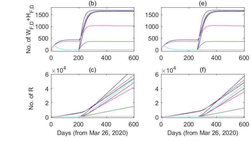
2

1. Introduction

    Heilongjiang Province, located in the northeast of China, shares a 3000-kilometre border with Rus-
sia and has 25 border ports. After China took the lead in containing the epidemic, the province had
become one of the main regions in the world to be suffering the second outbreak because of a large in-
flow of people from abroad [1]. No new or suspected infected cases had been reported in Heilongjiang
Province, China since March 10, 2020, and all confirmed cases were cured on March 26, 2020. How-
ever, there were 69 confirmed local cases in the province from April 11 to April 27, 2020, accounting
for 68 percent of the country’s total cases [2].
    The main reason for the second outbreak in Heilongjiang Province may be the surge in the number
of people imported from abroad. Suifenhe is a border town of just 70,000 people in Heilongjiang
Province, China. Taking Suifenhe border port in the province as an example, an average of 178 people
entered the city every day from March 26 to April 4, and the number reached a peak value 495 on
April 4, 2020 [2]. It is far beyond the prevention and control capacity of Suifenhe town. In addition,
with increasing severity of epidemic in foreign countries, General Administration of Civil Aviation of
China (CAAC) implemented the ’five ones’ flight policy. It means that each domestic airline company
can only reserve one route to each country, and that each route can not operate more than one flight
each week, so do foreign airlines [3, 4]. Meanwhile, the Chinese government adopted the diversion
policy on some major entry ports, except for Suifenhe port [5], which also brought great pressure on
epidemic prevention and control in the province.
    Therefore, Chinese and Russian governments have decided to temporarily close Suifenhe port to
suppress the spread of epidemic since April 7, 2020 [6]. At the same time, some sections of Suifenhe
town were under traffic control in April 9 [7], then all communities were closed in April 11 [8] and
other related control policies were carried out in time [9]. On April 2, the epidemic prevention and
control headquarters of Heilongjiang Province issued the 14th announcement: strictly implementing
six measures of 100% and ’closed-loop’ control [10].
    However, there is still the epidemic risk from imported cases due to the complicated terrain, frequent
trade between China and Russia. Moreover, compared with the epidemic in China having been effec-
tively restrained, the fear to the severity of epidemic in Russia will make more people seek for a safer
region by entering China through Suifenhe port, and may increase the number of infected importing
people. At present, the border port has been closed about 10 months and maybe longer. The long-term
border closure in the port will further cause more people to decide illegal importing via taking risks.
And illegal imported cases may greatly increase the potential spreading risk of the epidemic since they
are much harder to be monitored in time. Therefore, a long-term border closure may cause a paradox
phenomenon in epidemic control. It indicates that it may be more difficult to block the epidemic for a
long-term border closure than that for a border reopening, which may cause new epidemic rebounds in
Heilongjiang Province. The features of the epidemic outbreaks in the province are sporadic in many
regions. For example, a new epidemic appeared in Dongning City on December 10, 2020, a national
first-level border ports in Heilongjiang Province [11]. On January 20, 2021, a total of 68 cases were
confirmed in a single day, and 85 new asymptomatic infected cases were reported in the province [12].
    Many dynamic models were proposed to study the spread of COVID-19 with imported cases, and

Mathematical Biosciences and Engineering                                          Volume 19, Issue 1, 1–33.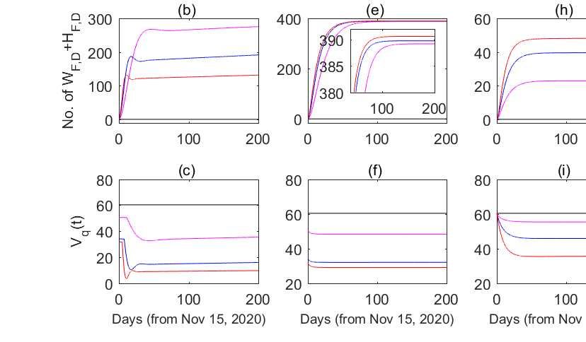
3
their results are useful to understand the impact of imported cases on epidemic outbreaks or design
effective border closure strategies in a short-term duration [13–31]. At present, there are more than
100 million confirmed cases worldwide, so we should investigate how to fight against imported novel
coronavirus for a future long-term duration. Moreover, it is necessary to explore whether the epidemic
rebounds are caused by the long-term border closure? If so, it is urgent to design a plan for reopening
the border in the province. Given the extensive border and numerous border ports in Heilongjiang
Province, it is essential to study the management of imported cases and control of COVID-19 epidemic
in the province.
In this paper, we extend the classical SEAIR compartmental framework to build a time switching
dynamical system to depict the transmission process of COVID-19 in three stages in Heilongjiang
Province, China. The model will combine with epidemic prevention and control strategies in the
province, including the government interventions (such as contact tracing and quarantine of both lo-
cal and importing populations, testing and diagnosing on infected cases, border closure), individual
compliance intensities (such as contract rate, the number of importing populations, the protection in-
tensity on nosocomial infection). Cross validation of parameter estimations was carried out by fitting
the model with eight time series of cumulative numbers in the province simultaneously to improve
its credibility. Then we found that illegal imported cases and imperfect protection intensity of noso-
comial infection are the main reasons for the second epidemic wave, and the actual border control
intensities are relatively effective in early control stage. Simulations showed the existence of a paradox
phenomenon under a long-term border closure. Hence combination with reducing economic losses,
people’s psychological burden, we define the daily reasonable number of legal importing population
by considering the resource limitations of hotel rooms and hospital beds. On this basis, the reopening
measure of border ports is designed for a long-term border control, which could inform public health
decision-makers carrying out the best border reopening strategy. Our results will not only help to con-
tain the spread of the epidemic in the province, but also can be referred for epidemic control in other
regions.
2. Method
2.1. Data
From the Health Commission of Heilongjiang Province, China, we noticed that there were no new
confirmed cases, no new suspected cases, no new confirmed importing cases from abroad, all 482
confirmed cases have been cured expect for 13 death cases, and all 16,389 close contacts have been
released from medical observation on March 26, 2020 in the province. And there is a similar situation
on July 1, 2020, but all 465 confirmed cases have been cured, and 4153 out of 4157 close contacts have
been released from medical observation. Thus the duration of the second wave of COVID-19 epidemic
in the province are approximately from March 26 to July 1, 2020. In this work, the eight time series of
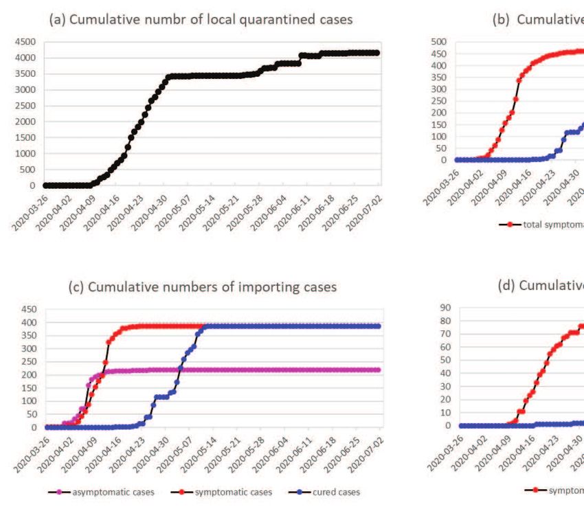
cumulative numbers related with COVID-19 in the duration are chosen as shown in Figure 1. It should
be mentioned that the cumulative number of local quarantined cases contains the cumulative numbers
of susceptible cases in quarantine together with exposed or infected cases in isolation.
Mathematical Biosciences and Engineering Volume 19, Issue 1, 1–33.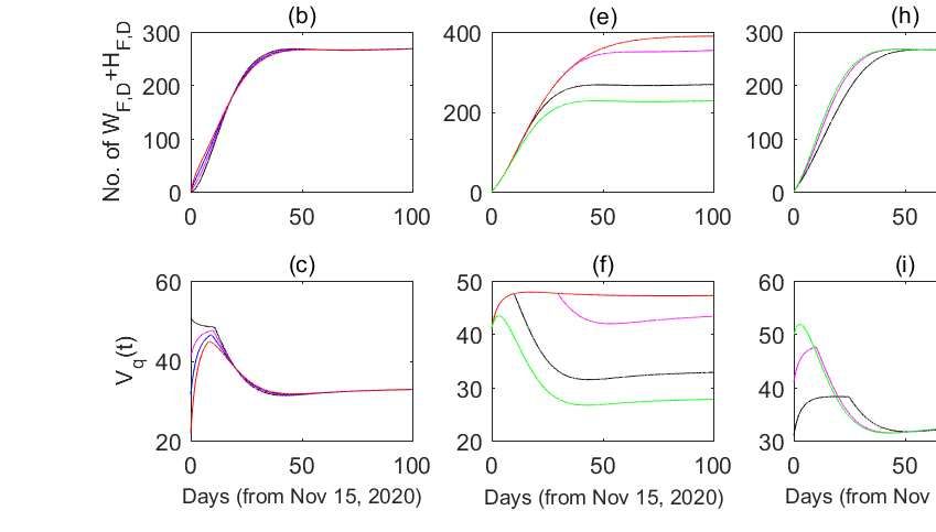
4

     Figure 1. The eight data series related with COVID-19 in Heilongjiang Province, China
     from March 26 to July 1, 2020. (a) Cumulative number of local quarantined cases (black),
     (b) cumulative numbers of local and importing symptomatic (red) and cured (blue) cases,
     (c) cumulative numbers of importing asymptomatic (magenta), symptomatic (red) and cured
     (blue) cases, (d) cumulative numbers of local symptomatic (red) and cured (blue) cases.

Mathematical Biosciences and Engineering                                    Volume 19, Issue 1, 1–33.
5

2.2. Model overview
    The Chinese government has imposed strictly centralized quarantine on legal returnees upon entry
since March 21, 2020, while there is no quarantine strategy for illegal returnees. Compared with
the strict movement restriction for local population under supervision, local population escaping from
supervision can move freely within the province to some extent. It indicates that there are different
population routes and intervention strategies for legal and illegal importing populations and for local
populations under supervision and without supervision. Hence the importing population is divided into
legal and illegal ones, while the local population is separated as freedom and control parts. We will
investigate the effects of importing cases and control strategies on the rebound of COVID-19 endemic
in Heilongjiang Province.
    Local population with freedom. Note that the incubation period accounts for a relative long
duration of the whole disease transmission period, and the exposed individuals in the late incuba-
tion period can transmit the virus into other susceptible individuals. There is a large proportion
of asymptomatic infectious individuals. We extend the transmission model Susceptible-Exposed in
the first stage (non-infectious)-Exposed in the second stage (infectious)-Infectious without symptoms-
Infectious with symptoms-Recover framework, by introducing variables S , E1 , E2 , A, I and R, respec-
tively.
    Legal importing population. Denote the daily number of legal importing population during border
opening as Vq (t). All the legal returnees upon entering the border are compulsively quarantined into the
nearby separated hotel rooms in the province, denoted as QF compartment. Note that all quarantined
individuals in the hotel rooms are forced to undergo multiple nucleic acid tests. According to the
first testing result, the legal importing population will be arranged into corresponding cabins. To be
exact, positive individuals without symptoms will be regarded as asymptomatic infected ones and to be
observed in hospitals (WF ), positive individuals with symptoms will be diagnosed as confirmed cases
to be treated in hospitals (HF ). If individuals’ testing results are negative within 14-day quarantine
period, then they will continue stay in QF , or until the end of quarantine period they will be released
into S . Similarly, for the second and subsequent nucleic acid tests, legal importing individuals will be
moved into the corresponding cabins (WF or HF ) once their testing results become positive during the
quarantine period.
    Illegal importing population. Some individuals may want to timely come across the border with-
out quarantine by choosing illegal importing way. Denote the daily number of illegal importing popu-
lation during border opening as V p (t). Note that there is no intervention strategy for illegal importing
population. It will be at any epidemic phases for illegal importing population entering the border and
mixing together with local population. Denote the proportions of illegal importing population being
the five epidemic phases as θS , θE1 , θE2 , θA , θI , respectively.
    Local population under control. Note that close tracking quarantine and testing strategy are
strictly implemented in the province. Local susceptible population closely contacting with infected
ones may be infected (qcβS Π/N) or not be infected (qc(1 − β)S Π/N), who will then be tracked and
quarantined into local quarantine compartments QD or QS , respectively. A proportion of exposed in
the second stage individuals (E2 ) and infectious without symptoms individuals (A) will be moved into
medicine observation wards (WD ). And a proportion of infectious with symptoms individuals (I) will
be diagnosed as confirmed cases and moved into medicine treatment wards (HD ).
    To explore the effect of importing population on the transmission of COVID-19 during different

Mathematical Biosciences and Engineering                                          Volume 19, Issue 1, 1–33.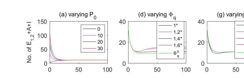
6
control stages, here we introduce three time intervals (here T 0 ≤ t < T 1 , T 1 ≤ t < T 2 , t ≥ T 2 ) as
the three phases I, II and III, respectively. Time points T 0 , T 1 and T 2 are the initial time (March 26th
2020), the actual switching time from border opening to one border closure intensity (April 7th 2020)
and the further possible switching time from the border closure intensity to another closure intensity,
respectively.
Actually, border closure strategy may change the behavior of individuals originally intend to enter
the border legally or illegally. A proportion of individuals intend to enter legally will choose to enter
illegally during border closure. And the number of legal and illegal importing individuals during
phases II and III may decrease by certain percentages, denoted by αi and α̂i (i = p, q), respectively.
Especially, a long-term border closure can cause more people to choose illegal importing by taking a
risk, so we assume that the maximum number of importing population in phase III will be increased to
fq and f p times that in the first two phases, respectively. Then we define the legal and illegal importing
populations in the three stages as follows
(Vq0 − Vqb )e−rq t + Vqb , i f T 0 ≤ t < T 1 ,
Vq (t) = (1 − αq )((Vq (T 1 ) − Vqb )e−rq (t−T1 ) + Vqb ), i f T 1 ≤ t < T 2 ,
(1 − α̂q )((Vq (T 2 ) − fq Vqb )e−rq (t−T2 ) + fq Vqb ), i f t ≥ T 2 ,
and
(V p0 − V pb )e−r p t + V pb , i f T 0 ≤ t < T 1 ,
V p (t) = (1 − α p )((V p (T 1 ) − V pb )e−r p (t−T1 ) + V pb ), i f T 1 ≤ t < T 2 ,
(1 − α̂ p )((V p (T 2 ) − f p V pb )e−r p (t−T2 ) + f p V pb ), i f t ≥ T 2 .
Moreover, we assume that the percentages of illegal importing population for each infection state
are the same during the first two sages for simplicity. To investigate the severity of the epidemic in
neighboring countries on the disease rebound in the province, we assume that the percentages of illegal
importing population being infected ones increase to fθ θ j0 ( j = E1 , E2 , A, I) in phase III. Then we define
θ j0 , i f T 0 ≤ t < T 2 ,
(
θj = j = E1 , E2 , A, I,
fθ θ j0 , i f t ≥ T 2 ,
and
θS 0 , i f T 0 ≤ t < T 2 ,
(
θS =
1 − fθ (θE10 + θE20 + θA0 + θI0 ), i f t ≥ T 2 .
In addition, we define
0, i f T 0 ≤ t < T 1 ,
(
ε=
1, i f t ≥ T 1 ,
where ε being equal to 0 and 1 are used to depict the border opening and closure, respectively.
Mathematical Biosciences and Engineering Volume 19, Issue 1, 1–33.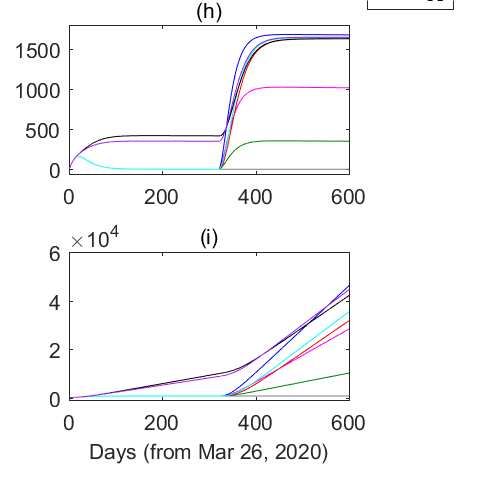
7
Illegal Importing population Legal
ܸ ǡ ߠ ǡ ݆ ൌ ܵǡ ܧଵ ǡ ܧଶ ǡ ܣǡ ܫ from abroad ሺͳ െ ߝሻܸ
Freedom Control
ߟܳௌ
ݒி ݇ே ߟܳி ܳௌ
ߠௌ ሺܸ
ߝܸ ሻ
ܵ ͳ ܿݍെ ߚ ܵȫȀܰ
ͳ െ ܵߚܿ ݍȫ ܵߚܿݍȫȀܰ ܳ ܳி
ߠாଵ ሺܸ
ߝܸ 澼 ܧଵ ݒ ݇ ܳ ݇ௐ ݒி ܳி
ݒ ͳ െ ݇ ܳ
ߜܧଵ
ߠாଶ ሺܸ ݉ாଶ ܧଶ
ߝܸ ሻ ܧଶ ܹ ݒி ݇ு ܳி ܹி
ߩ݇ ܧଶ
݉ ܣ
ߠ ሺܸ ݄ܹி
ߝܸ ሻ ܣ ܪி ݎௐ ܹி
ߩ ͳ െ ݇ ܧଶ ݎௐ ܹ ݄ܹ ݎு ܪி
ߠூ ሺܸ ݉ூ ܫ ݎு ܪ
ߝܸ ሻ ܫ ܪ ܴ
ݎ ܣ ݎூ ܫ
Figure 2. A flow diagram of model (2.1) adopted in this study for illustrating the imported
cases on the second outbreak of COVID-19 epidemic in Heilongjiang Province, China. Solid
and dashed blue lines are the legal and illegal importing routes, respectively. The freedom
and control plates means the corresponding populations being out of supervised and super-
vised, respectively. Variable ε being equal to 0 or 1 indicates the border port is opened
or closed, respectively. Solid red and black lines are population progression routes. Red,
black and brown dashed lines are disease transmission routes, the quarantining routes for in-
tensive contact tracing and the testing routes of freedom infectious individuals, respectively.
Magenta dashed (or dot-dashed) lines are the transfer routes among local (or importing) quar-
antined individuals and infected ones in hospitals.
Mathematical Biosciences and Engineering Volume 19, Issue 1, 1–33.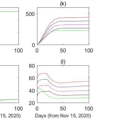
8
Based on above assumptions and the flow diagram in Figure 2, we build the model as follows
((1−q)β+q)cS Π
= θ + εV + kN vF ηQF + ηQS ,
′
S S V p (t) q (t) − N
Π
(1−q)βcS
E1 = θE1 V p (t) + εVq (t) + − δE1 ,
′
N
E2 = θE2 V p (t) + εVq (t) + δE1 − ρE2 − mE2 E2 ,
′
= θ + εV + kA ρE2 − rA A − mA A,
′
A A V p (t) q (t)
I = θI V p (t) + εVq (t) + (1 − kA )ρE2 − rI I − mI I,
′
Q′F = (1 − ε)Vq (t) − (kW + kH + kN η)vF QF ,
′
Π (2.1)
QD = qcβS N
− vD QD ,
Π
QS = qc(1−β)S − ηQS ,
′
N
WF = kW vF QF − rW WF − hWF ,
′
WD = kD vD QD + mE2 E2 + mA A − rW WD − hWD ,
′
HF = kH vF QF + hWF − rH HF ,
′
HD = (1 − kD )vD QD + hWD + mI I − rH HD ,
′
R′ = r A + r I + r (W + W ) + r (H + H ),
A I W F D H F D
with N = S + E1 + E2 + A + I + QF + QD + QS + WF + WD + HF + HD + R and Π = I + u1 A + u2 E2 +
u3 (WF + WD ) + u4 (HF + HD ). In fact, the item Π indicates all possible infection sources of the disease.
The items (1 − ε)Vq and V p + εVq are the actual daily number of legal and illegal importing population,
respectively. The detailed description of all variables and parameters in Figure 2 and model (2.1) are
shown in Tables 1, 2 and 3.
Table 1. Descriptions, initial values and sources of state variables for model (2.1).
Variable Description Initial value[(95% CI), Std] Source
S No. of susceptible individuals 18854[(1.8845,1.8863)e4, 626.83] Estimated
E1 No. of non-infectious exposed individuals 0 Assumed
E2 No. of infectious exposed individuals 0 Assumed
A No. of asymptomatic infectious individuals 0 Assumed
I No. of symptomatic infectious individuals 0 Assumed
QF No. of importing quarantined individuals 203 Data
QD No. of local quarantined individuals being infected 0 Data
QS No. of local quarantined individuals being susceptible 0 Data
WF No. of importing asymptomatic infectious individuals in hospitals 0 Data
WD No. of local asymptomatic infectious individuals in hospitals 0 Data
HF No. of importing symptomatic infectious individuals in hospitals 2 Data
HD No. of local symptomatic infectious individuals in hospitals 0 Data
R No. of recovered individuals 0 Data
Mathematical Biosciences and Engineering Volume 19, Issue 1, 1–33.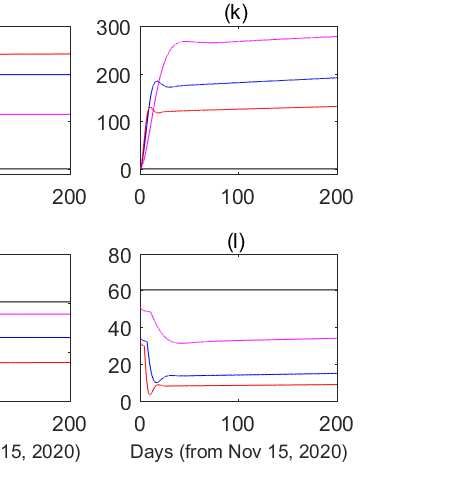
9

      Table 2. General parameter descriptions, values(Std), 95% CI and sources for models (2.1).
Para. Description                                                              Value(Std)           95% CI          Unit          Source
                                                                                                                   −1      −1
c    Contact rate                                                          5.1315(2.1453e-1)     (5.1286,5.1346) p day          Estimated
β    Probability of transmission per contact                             0.0024992(9.6232e-05) (2.4978,2.5005)e-3 p−1 day−1 Estimated
u1   Adjustment factor of contact rate with asymptomatic infectious 0.89511(8.6459e-2) (8.9389,8.9629)e-1           N/A         Estimated
     individuals
u2   Adjustment factor of contact rate with infectious exposed indi- 0.60683(1.4720e-2) (6.0662,6.0702)e-1          N/A         Estimated
     viduals
u3   Adjustment factor of contact rate with asymptomatic infectious        1.1521(4.7558e-2)     (1.1515,1.1528)    N/A         Estimated
     individuals in hospitals
u4   Adjustment factor of contact rate with symptomatic infectious         1.1339(2.8536e-2)     (1.1335,1.1343)    N/A         Estimated
     individuals in hospitals
δ    Transition rate from non-infectious exposed individuals to the              1/5(/)                 /          day−1           [37]
     infectious exposed ones
ρ    Transition rate from infectious exposed individuals to the infec-           1/3(/)                 /          day−1           [37]
     tious ones
η    Releasing rate of the quarantined uninfected individuals into the          1/14(/)                 /          day−1           [33]
     wider community
rA   Natural recovery rate of asymptomatic infectious individuals              0.1497(/)                /          day−1           [35]
rI   Natural recovery rate of symptomatic infectious individuals               0.1029(/)                /          day   −1
                                                                                                                                   [35]
                                                                                                                         −1
rW   Recovery rate of asymptomatic infectious individuals in hospi- 0.069457(5.3092e-4) (6.9450,6.9465)e-2 day                  Estimated
     tals
rH   Recovery rate of symptomatic infectious individuals in hospi- 0.081665(9.4146e-4) (8.1651,8.1677)e-2 day−1                 Estimated
     tals
q    Quarantined rate of exposed individuals                              0.10366(3.0272e-3) (1.0362,1.0370)e-1 day−1           Estimated
vF   Test rate of importing quarantined individuals                               1/2                   /          day−1           Data
                                                                                                                         −1
vD   Test rate of local quarantined individuals                           0.280244(2.9656e-3) (2.8020,2.8028)e-1 day            Estimated
kA   Transition probability of asymptomatic infectious individuals               0.6(/)                 /          day   −1
                                                                                                                                   [34]
     from exposed ones
kW   Percentage of quarantined importing individuals being asymp- 0.024348(4.3612e-4) (2.4342,2.4354)e-2            N/A         Estimated
     tomatic infected
kH   Percentage of importing quarantined individuals being con- 0.018201(4.7973e-4) (1.8194,1.8207)e-2              N/A         Estimated
     firmed cases
kN   Percentage of quarantined importing individuals being suscep-            0.957451(/)               /           N/A         1 − kW − kH
     tible
kD   Percentage of local quarantined individuals being asymp- 0.85281(3.5164e-2) (8.5232,8.5330)e-1                 N/A         Estimated
     tomatic infected
mE2 Diagnose rate of exposed infectious individuals                       0.18111(1.2844e-2) (1.8093,1.8129)e-1 day−1           Estimated
                                                                                                                         −1
mA Diagnose rate of asymptomatic infectious individuals                   0.18688(6.2376e-3) (1.8679,1.8696)e-1 day             Estimated
mI   Diagnose rate of symptomatic infectious individuals                  0.37121(1.9502e-2) (3.7094,3.7149)e-1 day−1           Estimated
                                                                                                                         −1
h     Transition rate from asymptomatic infectious individuals in 0.20811(1.7137e-3) (2.0809,2.0814)e-1 day                     Estimated
      hospitals to confirmed cases
p: person.

Mathematical Biosciences and Engineering                                                                    Volume 19, Issue 1, 1–33.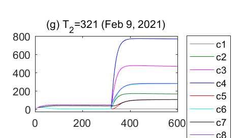
10

        Table 3. Importing related parameter descriptions, values(Std), 95% CI and sources for
        models (2.1).
  Para. Description                                                          Value(Std)                  95% CI         Unit Source
  θS     Percentage of illegal importing individuals being susceptible    0.8224(2.8054e-1) (8.2163,0.8.2240)e-1 N/A Estimated
  θE1 Percentage of illegal importing individuals being non-infectious 0.0396(1.7152e-2)         (3.9548,3.9595)e-2     N/A Estimated
      exposed
  θE2 Percentage of illegal importing individuals being infectious ex- 0.0360(2.5274e-2)         (3.5931,3.6000)e-2     N/A Estimated
      posed
  θA     Percentage of illegal importing individuals being asymptomatic 0.0252(2.2437e-2) (2.5174,0.02.5236)e-2 N/A Estimated
         infectious
  θI     Percentage of illegal importing individuals being symptomatic 0.0768(1.9134e-2)         (7.6722,7.6775)e-2     N/A Estimated
         infectious
  V p0 Introducing rate of illegal importing individuals at the initial 5.9726(3.4430e-1)             (5.9679,5.9775)   day−1 Estimated
       time
  Vq0 Introducing rate of legal importing individuals at the initial time 20.371(9.4832e-1)           (2.0358,2.0384)   day−1 Estimated
  V pb Maximum introducing rate of illegal importing individuals un- 20.181(1.8905e-1)                (2.0178,2.0184)        Estimated
       der the policy
  Vqb Maximum introducing rate of legal importing individuals under        57.496(2.0989)             (5.7468,5.7526)   day−1 Estimated
      the policy
  r1     Exponential increasing rate of introducing rate for illegal im- 0.043606(9.7476e-4) (4.3592,4.3619)e-2         N/A Estimated
         porting
  r2     Exponential increasing rate of introducing rate for legal import- 0.074462(9.4035e-4) (7.4450,7.4475)e-2       N/A Estimated
         ing
  Para. Description                                                                       Value range                   Unit Source
  αi     Compliance rate of individuals on border closure in phase II,                       [0, 1]                     N/A Assumed
         i = p, q for illegal or legal situation
  α̂i    Compliance rate of individuals on border closure in phase III,                      [0, 1]                     N/A Assumed
         i = p, q for illegal or legal situation
   fi    Adjustment factor on the maximum number of importing indi-               related to the epidemic               N/A Assumed
         viduals in phase III, i = p, q
   fθ    Adjustment factor on the proportion of illegal importing indi-           related to the epidemic               N/A Assumed
         viduals in phase III

Mathematical Biosciences and Engineering                                                                      Volume 19, Issue 1, 1–33.
11
Next, model (2.1) will used to reflect the effects of legal and illegal importing populations on the
transmission of the disease in Heilongjiang Province, China. We will first fitting the model to the eight
data categories and assess the transmission risk of the disease. Then we will investigate the possible
reasons for the second outbreak of the disease, and assess the effectiveness of early border strategies.
Especially, we explore a potential paradox or risk for long-term border closure if there are still serious
epidemics in some neighbour countries. Thus to avoid the potential risk, we finally explore the border
reopening measure under limiting resources for disease control.
3. Results
3.1. Risk assessment
The basic reproduction number R0 means the average number of individuals infected by the intro-
duction of a single infected one in the whole susceptible population. According our data collection
of the province, there is no new dead case from COVID-19 during the second outbreak. Thus under
the assumptions of no importing population and ignoring disease-induced death rate, there exists a
disease-free equilibrium for the model. Then we first calculate the effective reproduction number Rt by
using the next generation matrix method [32], as shown in Appendix A. From Eq (S4) in Appendix A,
the formula of Rt is a function with respect to time t, and it exists the term S (t)/N(t). Next if let t = 0,
then we can directly obtain the formula of R0 . Note that in the beginning of the disease rebound, it is
reasonable to assume that the initial number of susceptible population (i.e., S (0)) would approximate
to the number of total populations (i.e., N(0)), then the term S (0)/(N(0) can be simplified as one. By
removing the term S (t)/N(t) in Eq. (S4), we can obtain the formula of R0 as
R0 = R01 + R02 + R03 + R04 + R05 . (3.1)
It should be mentioned that R01 , R02 , R03 , R04 and R05 indicate the average number of individuals
infected by the introduction of a single infected individual of I, A, E2 , WF or WD and HF or HD in the
whole susceptible population, respectively. The detailed calculation process are shown in Appendix A.
3.2. Parameters
All parameters in model (2.1) can be divided into deterministic and estimated ones. We firstly
fix the deterministic parameters and the initial values from official survey reports, previous literatures
and the data information to reduce the complexity as show in Tables 1 and 2. The latent periods
in E1 and E2 stages are fixed as 5 and 3 days, respectively, i.e., δ = 1/5 and ρ = 1/3 [37]. The
testing rate of quarantined legal importing individuals and the releasing rate of uninfected individuals
under quarantine are fixed as vF = 1/2 and η = 1/14, respectively [33]. Notice that there is a quick
response to the second wave of COVID-19 epidemic in Heilongjiang Province and timely medical
supplies from other provinces, and there is no death cases from March 26 to July 1, 2020, so we ignore
the disease induced death rate in hospitals. The recovery rates of asymptomatic and symptomatic
infectious individuals are fixed as rA = 0.1497 and rI = 0.1029, respectively [35]. And the transition
probability from E2 to A is fixed as kA = 0.6 [34]. According to the data information, we fix the
initial values of QF and WF as 203 and 2, respectively. Since on March 26, 2020, there is no newly
confirmed symptomatic and asymptomatic cases, all local confirmed or quarantined cases are cured or
Mathematical Biosciences and Engineering Volume 19, Issue 1, 1–33.12
removed from close medical observation, respectively, so we reset initial cumulative numbers of local
quarantined, reported symptomatic and cured cases and other initial components being zero.
(a) Cumulative number of local quarantined cases (b) Cumulative numbers of importing and local cases
6000 600
4000 400
2000 200
0 0
0 50 100 150 0 50 100 150
(c) Cumulative numbers of importing cases (d) Cumulative numbers of local cases
600 100
400
50
200
0 0
0 50 100 150 0 50 100 150
Days (from Mar 26, 2020) Days (from Mar 26, 2020)
Figure 3. Goodness fitting results and validations of model (2.1) with the eight cumulative
data categories from March 26 to July 1, 2020 and from July 2 to Aug 22, 2020 for Hei-
longjiang Province, China. The color curves or circles are the goodness fitting results or the
corresponding cumulative data, respectively. The cumulative data used in (a), (b), (c) and (d)
are the same as the ones in Figure 1(a), (b), (c) and (d), respectively.
To estimate the values, standard deviations (Std) and 95% CI of the index parameters and initial
value of susceptible individuals (see Tables 1, 2 and 3), we simultaneously fit the proposed model (2.1)
to the eight cumulative data categories from March 26 to July 1, 2020 (see Figure 1) by carrying out
the Markov Chain Monte Carlo (MCMC) procedure [36]. In Figures 3 and 4, the best fitting results
are marked as color curves. The same color circles represent the corresponding data from March 26 to
July 1, 2020, while the color curves between July 2 to Aug 22, 2020 are used to verify our estimation
and predict the trends of solution curves. Specifically, the black, magenta, red and blue solid circles
(or curves) represent the cumulative number of local quarantined individuals, reported asymptomatic,
reported symptomatic and cured cases (or the best fitting results), respectively. Moreover, the best
fitting results and their 95% CI curves are shown in Figure 4. The yellow and cyan curves denote the
95% upper and lower confidence limits. In addition, the trends of the eight cumulative data are flat due
to almost no change on those data between July 2 to Aug 22, 2020, so we do not show them in the
figures.
It is worth mentioning that the eight time series of data are used to fit the model simultaneously,
which can help to cross-validating the estimation results and improve their credibility. It is difficult
to fit well the model with the eight time series of data simultaneously in a long time interval. From
Figures 3 and 4, although our fitting results are a little higher than their real data during the steady
states since some strong interventions are carried out after April 7. However, the fitting results are
well during the initial stage of the second outbreak. Moreover, we assume a priori distribution for each
Mathematical Biosciences and Engineering Volume 19, Issue 1, 1–33.13
(a) (b-1) (b-2) (c-1)
6000 600 600 400
300
4000 400 400
200
2000 200 200
100
0 0 0 0
0 100 200 0 100 200 0 100 200 0 100 200
(c-2) (c-3) (d-1) (d-2)
500 500 200 200
400 400
150 150
300 300
100 100
200 200
50 50
100 100
0 0 0 0
0 100 200 0 100 200 0 100 200 0 100 200
Days (from Mar 26, 2020) Days (from Mar 26, 2020) Days (from Mar 26, 2020) Days (from Mar 26, 2020)
Figure 4. Goodness fitting results and validation of model (2.1) with the eight cumulative
data categories from March 26 to July 1 and from July 2 to Aug 22 2020, and their 95% CI
from March 26 to August 22, 2020 in Heilongjiang Province, China. The eight subplots (a),
(b-1) to (b-2), (c-1) to (c-3) and (d-1) to (d-2) are the corresponding results related with the
eight cumulative data in Figure 1 (a), (b), (c) and (d), respectively. The color circles are the
cumulative data and the black cures are the goodness fitting results. The yellow and cyan
curves denote the 95% upper and lower confidence limits.
Mathematical Biosciences and Engineering Volume 19, Issue 1, 1–33.14
parameter to be estimated based on their available information. That is to say, a penalized MCMC
method are carried out to select the optimal parameter values and their 95% CI within the reasonable
ranges which were obtained from official survey reports and previous literatures. In addition, we can
obtain the basic reproduction number R0 = 0.7882 for the second wave of COVID-19 in Heilongjiang
Province based on the above results. Later, the values of R0 will be as one of the important aspects to
assess the effectiveness of early control strategies in the province.
3.3. Reasons for the second outbreak
The number of hiding infected individuals without effective supervision and control (i.e., E1 + E2 +
A + I) implies the potential transmission risk of COVID-19 epidemic from importing population. The
number of infected cases in hospitals (i.e., WF + WD + HF + HD ) indicate the capacity of testing,
diagnosing and treatment of the disease. The number of local infected cases in hospitals (i.e., WD + HD )
partly reflect the effect of illegal importing population and control strategies on the local epidemic. The
number of infected individuals (i.e., E1 + E2 + A + I + WF + WD + HF + HD ) and the total number of
cured cases (i.e., R) indicate the time-varying epidemic scale and its final size, respectively. The four
indexes may be used in the following parts, ordered by index 1,2,3 and 4 for simplicity.
To explore the possible reasons for the second outbreak of COVID-19 in Heilongjiang, China, we
firstly assume that it is a virus-free environment in the province, so the initial values are reset as zero,
besides the initial susceptible population simply fixed as its previous estimation value. The adjustment
factors u3 and u4 reflect the protection intensity of susceptible individuals in hospitals, so their values
being zero or not indicate the perfect or imperfect protection intensity. Notice that legal and illegal
importing populations (Vq∗ (t), V p∗ (t)), the percentages of illegal importing population being different
subgroups θi (i = S , E1 , E2 , A, I) and the protection intensity ui (i = 3, 4) will impact the rebound of
COVID-19 in the province. For convenience, u3 and u4 are fixed as the pervious estimation values to
represent imperfect protection intensity. Therefore, we consider the following five special scenarios
with perfect (i.e., u3 = u4 = 0) or imperfect (i.e., ui , 0, i = 3, 4) protection intensity.
Case 1: No importing from aboard, i.e., V p∗ (t) = 0, Vq∗ (t) = 0;
Case 2: Only susceptible importing from aboard, i.e., V p∗ (t) = V p (t), Vq∗ (t) = Vq (t), θS = 1;
Case 3: Only legal importing from aboard, i.e., V p∗ (t) = 0, Vq∗ (t) = V p (t) + Vq (t);
Case 4: Only illegal importing from aboard, i.e., V p∗ (t) = V p (t) + Vq (t), Vq∗ (t) = 0;
Case 5: Both legal and illegal importing from aboard, i.e., V p∗ (t) = V p (t), Vq∗ (t) = Vq (t).
It follows from Figure 5 that there is no rebound of COVID-19 if there is no importing or only sus-
ceptible individuals import from aboard no matter with perfect protection intensity or not (Cases 1 and
2 shown by cyan and magenta curves). If all importing population choose to legally enter the border,
then the perfect protection intensity will not cause the rebound of the epidemic, while the imperfect
protection intensity will lead to the slight rebound on the number of infected individuals under super-
vision or not, with the peak values at about 32 days and 50 days around 7 cases, respectively (Case
3 shown by blue curves in Figure 5). However, if all importing population illegally enter the border,
the peak values of infected individuals under supervision or not at about 12 or 15 days will increase
over seven times compared with the peak values in Case 3 with imperfect protection intensity (Case 4
shown by red curves in Figure 5). For the general case 5, if there are both ileal and illegal importing
populations as the previous estimation, the peak values of infected individuals under supervision or not
Mathematical Biosciences and Engineering Volume 19, Issue 1, 1–33.15
(a) (b)
40 40
case 1 with u 3 =u4 =0
case 1 with u 3 ,u 4 ( 0)
35 35
case 2 with u 3 =u4 =0
case 2 with u 3 ,u 4 ( 0)
30 30
case 3 with u 3 =u4 =0
case 3 with u 3 ,u 4 ( 0)
No. of E1 +E2 +A+I
25 25
case 4 with u 3 =u4 =0
No. of WD+HD
case 4 with u 3 ,u 4 ( 0)
20 case 5 with u 3 =u4 =0 20
case 5 with u 3 ,u 4 ( 0)
15 15
10 10
5 5
0 0
0 50 100 150 200 0 50 100 150 200
Days (from Mar 26, 2020) Days (from Mar 26, 2020)
Figure 5. Possible reasons for the second outbreak of COVID-19 in Heilongjiang Province,
China. The baseline parameter values are fixed as in Tables 2 and 3. Initial components are
fixed as zero, except for S 0 = 18854.
at about 14 or 16 days will increase less than 1.5 times compared with the peak values in case 3 with
imperfect protection intensity (see black curves in Figure 5). Especially, in Case 4 (or 5), there exist
slightly differences on the solution curves between perfect and imperfect protection intensity around 20
(or 15) days before, then the differences of solution curves will gradually increase and then gradually
decreased. All the black curves represent the baseline solutions according our previous parameter esti-
mation. Thus the illegal importing population and imperfect protection intensity are the main reasons
for the second outbreak of COVID-19 epidemic in the province.
3.4. Effectiveness of early control strategies
The early border control strategies mainly consist of the coercive government interventions, such
as intensive contact tracing and quarantine q, testing and diagnosing infected cases mi (i = E2 , A, I),
border closure strategy and individual compliance intensity, including wearing a mask and keeping
social distance to change the contract rate c and varying the number of illegal and legal importing
populations Vi (t)(i = p, q). So those parameter values can used to depict the intensity of early border
control strategies. In fact, the estimation of those parameter in subsection 3.2 determines the actual
intensity of early border control strategies. In order to investigate whether the early border control
strategies in the province are effective or not, we first regard them as the baseline situation. In Figures
S1, S2, S3, S4 and S5, we compare the effects of both strengthening and weakening those parameter
values with the baseline situation on the values of the four indexes, which can assess the effectiveness
of controlling COVID-19 epidemic. In addition, model (2.1) involves the border control strategies.
According to the definition of the basic reproduction number R0 , its value can be used to assess the
Mathematical Biosciences and Engineering Volume 19, Issue 1, 1–33.16
disease transmission risk and the effectiveness of control strategy in the early stage. By using the
parameter estimation values and the known parameter values, we obtain R0 = 0.7882 < 1 for the
second wave of epidemic, which also indicates the effectiveness of its early control strategy.
In summary, it follows from either the basic reproduction number or Figures S1, S2, S3, S4 and
S5 that the actual border control intensities in Heilongjiang Province are relative effective in the early
border control stage, and the rebound of COVID-19 epidemic will be worsen once the actual border
control strategies are relaxed. See Appendix B for more details about the explanation each one of
Figures S1, S2, S3, S4 and S5.
3.5. Possible risk for long-term border closure
The COVID-19 epidemic in China has been effectively restrained due to effective control strategies
adopted by the Chinese government and the better individual compliance on wearing masks and keep-
ing social distance to degrade exposure rate, while some epidemic in the neighbouring countries, such
as Russia may not yet controlled or even get worse. Then the fear to the epidemic will make more
Chinese people study or working in Russia seek for a safer region by entering China through Suifenhe
port in Heilongjiang Province. However, the long-term border closure in the port will further lead to
more people deciding to take risks and enter illegally. Also compared with legal imported cases, ille-
gal imported cases are much harder to be monitored in time which may greatly increase the potential
spreading risk of the epidemic. Moreover, the proportions of infected importing individuals may be
increased for the severity of epidemic in the neighbouring countries. It is critical to answer whether
a long-term border closure may cause a paradox phenomenon or not, in other words, whether it will
be much harder to block the epidemic for a long-term border closure than that for a border reopening.
To depict the long-term border closure, the maximum number of illegal importing population and the
proportions of them being different subgroups θi (i = S , E1 , E2 , A, I) are redefined by regulation param-
eters fi (i = p, q) and fθ in phase III. It is difficult to obtain their accurate parameter values. Since we
aim to explore the potential risks for the long-term border closure, the regulation parameters are fixed
as fi = 4(i = p, q) and fθ = 3 for simplicity. Thus we consider the following eight special scenarios
along with different switching time T 2 (= 103, 163, 223), as shown in Table 4 and Figure 6.
Table 4. Eight special scenarios for the long-term border control strategies.
Case I: T 0 ≤ t < T 1 II: T 1 ≤ t < T 2 III: t ≥ T 2 SVF SVC SV
1 strictly close, V p∗ = Vq∗ =0 0 0 0
2 close, α̂ p = α̂q = 0.8, V p∗ = V p + Vq 152.6 334.0 486.6
3 open with legal strictly close, close, α̂ p = α̂q = 0.4, V p∗ = V p + Vq 456.8 1001.0 1457.8
4
and illegal i.e., V p∗ = Vq∗ = 0 close, α̂ p = α̂q = 0, V p∗ = V p + Vq 761.1 1668.0 2429.1
importing,
5 i.e., V p∗ = V p , open, V p∗ = 0, Vq∗ = V p + Vq 107.5 1635.4 1743.0
6 Vq∗ = Vq open, V p∗ = V p , Vq∗ = Vq 278.6 1645.5 1924.2
7 open, V p∗ = 0, Vq∗ = V p + Vq open, V p∗ = 0, Vq∗ = V p + Vq 107.5 1635.4 1743.0
8 open, =
V p∗ V p , Vq∗
= Vq open, V p∗= V p , Vq∗
= Vq 278.6 1645.5 1924.2
SVF: the steady value of infected individuals without supervision (or with freedom), i.e., E1 + E2 + A + I; SVC: the steady value of
infected individuals with supervision (or with control) in hospitals, i.e., WF + WD + HF + HD ; SV: the steady value of infected individuals,
i.e., E1 + E2 + A + I + WF + WD + HF + HD .
Mathematical Biosciences and Engineering Volume 19, Issue 1, 1–33.17
Figure 6. The evaluation of a long-term border closure on COVID-19 epidemic in Hei-
longjiang Province, China. (a-c): T 2 = 198 (Oct 9, 2020); (d-f): T 2 = 259 (Dec 9, 2020);
(g-i): T 2 = 321 (Feb 9, 2021). The magenta, blue, red, cyan brown and black curves repre-
sent the corresponding solution curves of model (2.1) for the eight cases. In this work, the
items E1,2 and WF,D denote E1 + E2 and WF +WD , respectively. The baseline parameter values
and initial values are the same as in Tables 1, 2 and 3.
From Figure 6(a)–(c) and Table 4, there are eight cases for the solutions of the three indicators in
phases I, II and III. In phase II, it is clear that the strict border closure greatly contributes to prevent the
COVID-19 epidemic. A sustained and strict border closure in phase III will effectively suppress the
disease transmission. And SVF and SVC will greatly increase with reducing individual compliance
(α̂ p , α̂q ) on border closure in phase III. For some cases in phase III, SVF of border closure are larger
than that of border reopening (see Table 4 and Figure 6(a)). Compared with border reopening, the
existence of a paradox phenomenon in the long-term border closure not only may not help to suppress
the epidemic, but worsen the epidemic control. Comparing SVC and SV among cases 2 to 8, the border
reopening will greatly increase the infected individuals and then the required hospital beds and other
medical resources. Moreover, there are the same SVF, SVC and SV for cases 5 and 7 due to the model
(2.1) in phase III being the same with slight difference of initial values, and similar situation for cases
6 and 8. The three switching time T 2 in the simulations are chosen within the steady interval of phase
II, so for model 2.1 in phase III there are the same initial values, except for the initial state of recovery
Mathematical Biosciences and Engineering Volume 19, Issue 1, 1–33.18
being independent to other variables. Actually the solution curves in Figures 6(d) and (e) (or (g) and
(h)) are those in (a) and (b) moved forward by 2 (or 4) months. Especially, the actual SAV, SVC and
SV should be correspondingly within their intervals determined by the two extreme cases 4 and 6.
Although we may not know the actual switching time T 2 , it can still help us to uncover the potential
transmission risk and assess the final size, and then to make some advance preparations.
3.6. Border reopening measure under resource limitations
According to subsection 3.5, a long-term border closure will not only cause huge economic losses,
but also may bring much severer challenges on the control of COVID-19 epidemic in Heilongjiang
Province than that of border reopening with the worsening epidemic and people fearing to the epidemic
in Russia. Next we will explore how to effectively reopen Suifenhe port in Heilongjiang Province.
Since anti-epidemic resources, including the number of hotel rooms and hospital beds are usually
limited. In order to carry out orderly border reopening strategy, the potential required resources for
importing population per day should be satisfied by the local resources. That is to say, the number
of importing population per day should be determined by the locally available resources. For conve-
nience, Φq and Φh denote the total number of hotel rooms and the total number of hospital rooms,
respectively, while H1 or H2 denote the average maximum number of people who can be legally im-
ported per day due to limiting resources on hotel rooms or hospital rooms, respectively. Notice that
η−1 and max{1/rW + 1/h, 1/rH } represent the average duration of importing population being quaran-
tined and the average duration of infected cases being treated in hospitals, respectively. Then Φq η
and Φh / max{ r1W + 1h , r1H } are the total available numbers of hotel rooms and hospital beds per day,
respectively. The items
qcS Π
and mE2 E2 + mA A + mI I + vD QD
N
correspondingly represent the numbers of hotel rooms and hospital beds being used per day. Notice
that
qcS Π
≈ Newquar (t) and mE2 E2 + mA A + mI I + vD QD ≈ Newhosp (t), (3.2)
N
where Newquar (t) and Newhosp (t) denote the daily new being quarantined and treated cases, respectively.
The item (kW + kH )vF QF represents the daily number of required hospital rooms. Based on the resource
limitations on hotel or hospital rooms, the average maximum number of people can be legally imported
per day can be calculated correspondingly as
qcS Π
Φq η −
N
or
Φh
− (mE2 E2 + mA A + mI I + vD QD ).
max{ r1W+ h1 , r1H }
Then we have
qcS Π
H1 = Φq η − (3.3)
N
and
Φh
(kW + kH )vF QF = − (mE2 E2 + mA A + mI I + vD QD ). (3.4)
max{ r1W+ 1h , r1H }
Mathematical Biosciences and Engineering Volume 19, Issue 1, 1–33.19
Letting the right side of the sixth equation in model (2.1) equal to zero yields
Vq
QF = . (3.5)
(kW + kH + kN η)vF
By substituting (3.5) into (3.4), solving equation (3.4) with respect to Vq yields
kW + kH + kN η Φh
H2 Vq = + + + .
− (m E2 E 2 m A A m I I v D Q D ) (3.6)
kW + kH max{ r1W + 1h , r1H }
To explore the threshold values of Φ∗q and Φ∗h such that the two anti-epidemic resources can be
efficiently used, solving H1 = H2 with respect to Φq or Φh obtains
H2 + qcSN Π
Φ∗ = η
,
q
H1
kW +kH +kN η +mE2 E2 +mA A+mI I+vD QD (3.7)
kW +kH
Φ∗h = .
max{ r 1 + 1h , r1 }
W H
The relation between model (2.1) and the two data sets are shown in equation (3.2) and our model
(2.1) can fit well with the eight data categories as in subsection 3.2. It is worth mentioning that the
model driven calculations about H1 , H2 , Φ∗q and Φ∗h in equations (3.3), (3.6) and (3.7) can also be
correspondingly replaced by the data driven ones via (3.2). Considering that the work in this section
is a prospective study on future border reopening strategies, there is no data resources about the daily
new to be quarantined and treated cases for border reopening. Thus here we choose to use the model
driven calculations in our following numerical simulations.
Some infected individuals may enter into the border, i.e., kW + kH , 0, if pre-entry testing is not
mandatory or testing accuracy is imperfect. Then we define the daily number of people allowed to
legally enter the border as
wH1 , i f min {H1 , H2 , H2 − H1 } > 0,
Vq (t) = wH2 , i f min {H1 , H2 , H1 − H2 } > 0, (3.8)
0, otherwise,
where w is an adjustment factor to avoid anti-epidemic resources crowding due to some unforeseen
circumstances in practice. The proportion of daily number of illegal importing population to that of
legal ones is denoted by qv , then we have
qv wH1 , i f min {H1 , H2 , H2 − H1 } > 0,
V p (t) = qv wH2 , i f min {H1 , H2 , H1 − H2 } > 0, (3.9)
V p0 , otherwise.
Especially, all legal importing individuals are susceptible, i.e., kW + kH = 0, kN = 1, if pre-entry test-
ing is mandatory and testing accuracy is perfect. Then we define the daily number of people entering
the border legally or illegally as
wH1 , i f H1 > 0, qv wH1 , i f H1 > 0,
( (
Vq (t) = V p (t) = (3.10)
0, otherwise, V p0 , otherwise.
Mathematical Biosciences and Engineering Volume 19, Issue 1, 1–33.20
In order to explore the effects of the proportion of legal importing population being susceptible kN ,
the number of illegal importing population V p (t), the regulatory factors of contact rates from protecting
compliance in hospitals ui (i = 3, 4), initial values (depicted by P0 ) and anti-epidemic resources Φi (i =
q, h) on the potential transmission risk and the occupied number of hospital beds when the border
reopening strategy is carried out in Suifenhe port. We analyze the sensitivity for varying one, two
and three of the above control parameters (kN , V p (t), ui ) separately based on the designed reopening
strategy, as shown in Figures 7, 8 and 9. According to the news reports about the numbers of hospital
rooms and medical beds on Suifenhe, the two resource parameters are set as Φq = 939 and Φh = 630.
All parameter values are the same as our previous estimations, except for the above noteworthy ones.
Specifically in Figures 7 and 8, besides of the target parameters, other noteworthy ones are fixed as
kN = 1, V p = u3 = u4 = 0, and the initial values are fixed as zero, except for S 0 = 18854. In Figure
9, besides of the target parameters, other noteworthy ones are fixed as kN = 0.9, V p = 0.05Vq , ui =
0.2ûi (i = 3, 4) and P0 = 10, where ûi are the estimation values of ui in Table 2.
Figure 7. Effects of varying one control parameter value (kN or V p (t)) on the border reopen-
ing of Suifenhe prot in Heilongjiang Province, China. (a-c): V p = u3 = u4 = 0; (d)-(f):
kN = 1, u3 = u4 = 0. The initial values and baseline parameter values are the same as in
Figures 5, and Φq = 939, Φh = 630.
Although there is no potential transmission risk, no occupied medical beds and a high number of
legal importing population for border reopening with ideal situations i.e., kN = 1, V p = u3 = u4 = 0 (see
black curves in Figure 7 (a-b) and (d-e)), it is difficult to simultaneously attain those perfect control
intensities in reality. There is the same results for kN = 1, V p = 0 and ui , 0(i = 3, 4), so here we
do not show its simulation results. From Figure 7 (a-c), no illegal importing together with perfect
protection intensity V p = u3 = u4 = 0 can successfully suppress the potential transmission risk even
Mathematical Biosciences and Engineering Volume 19, Issue 1, 1–33.21
Figure 8. Effects of varying two or three control parameter values (V p (t),kN ,u3,4 ) on the
border reopening strategy of Suifenhe prot in Heilongjiang Province, China. The black,
magenta, blue and red solution curves in (a-c) for (1, u3,4 ), (0.9, 0.2u3,4 ), (0.6, 0.5u3,4 ) and
(0.3, 0.8u3,4 ); in (d-f) for (0, 1), (0.05Vq , 0.9), (0.1Vq , 0.6) and (0.15Vq , 0.3); in (g-i) for
(0, u3,4 ), (0.05Vq , 0.2u3,4 ), (0.1Vq , 0.5u3,4 ) and (0.15Vq , 0.8u3,4 ), and in (j-l) for (0, 1, u3,4 ),
(0.05Vq , 0.9, 0.2u3,4 ), (0.1Vq , 0.6, 0.5u3,4 ) and (0.15Vq , 0.3, 0.8u3,4 ). The initial values and
baseline parameter values and are the same as in Figures 5.
Mathematical Biosciences and Engineering Volume 19, Issue 1, 1–33.22
for legal importing population with high infection proportion (i.e., low kN ). Also the increase of kN
can help to reduce the occupied number of medical beds in the first two months followed by tending to
the same steady values, and help to increase the daily number of legal importing population for border
reopening. From Figure 7 (d-f), the lower V p is benefit to reduce the potential transmission risk and
the number of occupied medical beds, and increase the daily number of legal importing population.
The improvement for control intensities through combining two or three parameters (here V p , kN , ui ) at
the same time can help to reduce the potential transmission risk and increase the daily number of legal
importing population to some extent, see Figure 8. In reality, on the one hand, we aim to reduce the
potential transmission risk and increase the number of legal importing population by improving control
intensities; on the other hand, the quantity of infected population under supervision should be lower
than the available medical beds to receive infected individuals in time, although there is no consistent
conclusion for its quantity with improving control intensities, see Figures 8.
Figure 9. Effects of varying initial values reflected by P0 and anti-epidemic resources Φi (i =
q, h) on the border reopening strategy of Suifenhe prot in Heilongjiang Province, China. Fix
E10 = E A0 = E I0 = P0 , E20 = 0.5P0 and P0 = 10 in (d-l). In (d)-(f), 1.2∗ represents Φq
replaced by 1.2Φq ; in (j)-(i), (1.4, 1.2)∗ represents Φq and Φh replaced by 1.4Φq and 1.2Φh ,
respectively. There are similar meanings for other items. The baseline parameter values and
are the same as in Figures 5.
It follows from Figure 9, varying the values of P0 and Φh can only impact the solution curves in the
earlier phase followed by tending to the same steady values. The stable solution curves for different
values of Φh coincide with the stable curves for the threshold values ΦSh (green) in Figure 9 (g-i). From
Figure 9 (d-f), the stable solution curves for the estimation values (black) is higher than that for the
threshold values ΦSq (green), and the corresponding stable solution curves will increase with increasing
Mathematical Biosciences and Engineering Volume 19, Issue 1, 1–33.23
Φq from 1 to 1.2, 1.4 multiplying by the actual hotel room number 939. However, the stable solution
curves will not been changed with unceasingly increasing the values of Φq from 1.4 to 1.6, times 939. It
indicates that in Suifenhe port, the quantity of actual available medical beds is more sufficient than that
of required ones compared with the required and available quantities of hotel rooms, and that there will
no help to reduce the potential transmission risk or increase the number of legal importing population
when successively increasing available hotel rooms make its number more than that of required ones.
In Figures 9 (j-l), the stable solution curves will increase with simultaneously increasing the hotel
room and medical bed numbers. Compared with Figures 9 (d-i), the simultaneously increasing the
anti-epidemic resources can only make a slight addition on the number of infected individuals without
supervision, but can help to increase the numbers of both infected individuals in hospitals and legal
importing population. It is worth mentioning that with increasing the hotel room number or medical
bed number based on the designed border reopening strategy, the quantity of the available medical
beds is always more than that of infected individuals under supervision, even when the number of
infected individuals may be increased to some extent, and that the allowable number of legal importing
population is increased. Hence, the designed border reopening process give an effective strategy of
reopening Suifenhe port with considering limitation resources.
4. Conclusions
The local transmission of COVID-19 seems to have been contained in China under unprecedented
public health interventions, while some epidemics in the neighbouring countries, such as Russia may
not yet controlled or even getting worse. The second wave of outbreak was aroused in several re-
gions owing to introducing some imported cases, such as Heilongjiang, Beijing and so on. Especially,
Suifenhe port of Heilongjiang Province undertook major imported cases after the strict policy of immi-
gration diversion in main entry ports by the government, and then the severe rebound of the epidemic
occurred in the province. It is necessary to investigate all possible reasons for the second outbreak of
the disease, and assess the effects of early border control strategies on the prevention of the disease.
It is intuitive that border closure in Suifenhe prot contributes to the restrain the rebound of epidemic
in the provinces. However, the fear to the severity of epidemic in Russia could make more people
seek for a safer region by illegally entering Heilongjiang Province, China, which could be worsen if
a long-term border closure will carry out in the border port. And illegal imported cases may greatly
increase the potential spreading risk of the epidemic since they are much harder to be monitored in
time. It is critical to explore the possible risk for the long-term border closure strategy, and then design
an effective border reopening measure with considering the limitation of anti-epidemic resources. To
answer above relative issues, we developed a time switching system to depict the transmission and
spread of COVID-19 in three different time phases. The daily numbers of legal and illegal importing
populations and the percentages of illegal importing population are depicted in three phases by intro-
ducing several adjustment parameters. The basic reproduction number are calculated as in (3.1), which
can be separated into five parts from the possible types of infected individuals. Notice that there were
no new or suspected infected cases for Heilongjiang Province and all confirmed cases have been cured
on March 26 and July 1, 2020, so the eight data categories in this duration are chosen to study the
effects of imported cases on the COVID-19 rebound and its control in the province. Cross validation
was carried out by fitting the model with eight time series of cumulative numbers simultaneously to
Mathematical Biosciences and Engineering Volume 19, Issue 1, 1–33.You can also read