Modelling the mass budget and future evolution of Tunabreen, central Spitsbergen
←
→
Page content transcription
If your browser does not render page correctly, please read the page content below
The Cryosphere, 16, 2115–2126, 2022
https://doi.org/10.5194/tc-16-2115-2022
© Author(s) 2022. This work is distributed under
the Creative Commons Attribution 4.0 License.

Modelling the mass budget and future evolution of Tunabreen,
central Spitsbergen
Johannes Oerlemans1 , Jack Kohler2 , and Adrian Luckman3
1 Institute
          for Marine and Atmospheric Research, Utrecht University, Princetonplein 5, 3585CC Utrecht, the Netherlands
2 Norsk Polarinstitutt, Hjalmar Johansengate 14, 9296 Trømso, Norway
3 Department of Geography, Swansea University, Singleton Park, Swansea, SA2 8PP, United Kingdom

Correspondence: Johannes Oerlemans (j.oerlemans@uu.nl)

Received: 20 May 2021 – Discussion started: 15 June 2021
Revised: 18 April 2022 – Accepted: 4 May 2022 – Published: 1 June 2022

Abstract. The 26 km long tidewater glacier Tunabreen is the       1   Introduction
most frequently surging glacier in Svalbard, with four doc-
umented surges in the past 100 years. We model the evolu-
tion of this glacier with a minimal glacier model (MGM), in       Tunabreen is a 26 km long tidewater glacier in central Spits-
which ice mechanics, calving, and surging are parameterized.      bergen (Fig. 1). It is the most frequently surging glacier in
The model geometry consists of a flow band to which three         Svalbard, with four documented surges during the past 100
tributaries supply mass. The calving rate is set to the mean      years (Flink et al., 2015; Luckman et al., 2015). The surges
observed value for the period 2012–2019 and kept constant.        occurred during 1924–1930 (advance 3 km), 1966–1971 (ad-
For the past 120 years, a smooth equilibrium line altitude        vance 2.1 km), 2002–2004 (advance 2 km), and 2016–2018
(ELA) history is reconstructed by finding the best possible       (advance 1.1 km). It appears that the frequency of surging has
match between observed and simulated glacier length. There        been increasing, with shorter duration of the periods of ad-
is a modest correlation between this reconstructed ELA his-       vance (Fig. 2). Analysis of crevasse patterns visible in high-
tory and an ELA history based on meteorological observa-          resolution satellite images has shown that surging is initiated
tions from Longyearbyen.                                          close to the glacier front and then propagates upward (Flink
   Runs with and without surging show that the effect of surg-    et al., 2015).
ing on the long-term glacier evolution is limited. Due to the        Svalbard has a wide spectrum of surging glaciers, with
low surface slope and associated strong height–mass-balance       surge periods ranging from a couple of decades to (pre-
feedback, Tunabreen is very sensitive to changes in the ELA.      sumably) a few hundred years (Lefauconnier and Hagen,
For a constant future ELA equal to the reconstructed value        1991). Many of the larger tidewater glaciers on Svalbard
for 2020, the glacier front will retreat by 8 km during the       do surge regularly (a precise percentage is not known).
coming 100 years. For an increase in the ELA of 2 m a−1 ,         Glaciers with well-documented surge behaviour in a similar
the retreat is projected to be 13 km, and Tunabreen becomes       size class to Tunabreen are for instance Kongsvegen (length
a land-terminating glacier around 2100.                           ≈ 25 km, slope ≈ 0.028), Comfortlessbreen (length ≈ 16 km,
   The calving parameter is an important quantity: increas-       slope 0.042), and Monacobreen (length ≈ 40 km, slope
ing its value by 50 % has about the same effect as a 35 m         ≈ 0.027). The characteristic slope of Tunabreen (≈ 0.032)
increase in the ELA, with the corresponding equilibrium           is within the usual range of larger tidewater glaciers. The
glacier length being 17.5 km (as compared to 25.8 km in the       observed long-term (multi-annual) calving rate is relatively
reference state).                                                 high (≈ 270 m a−1 ), but it should be noted that calving rates
   Response times vary from 150 to 400 years, depending on        vary enormously across the archipelago (Blaszczyk et al.,
the forcing and on the state of the glacier (tidewater or land-   2009). The surges of Tunabreen appear to be initiated on
terminating).                                                     the lowest part of the glacier and propagate upward, which
                                                                  is not uncommon for surging tidewater glaciers in Svalbard

Published by Copernicus Publications on behalf of the European Geosciences Union.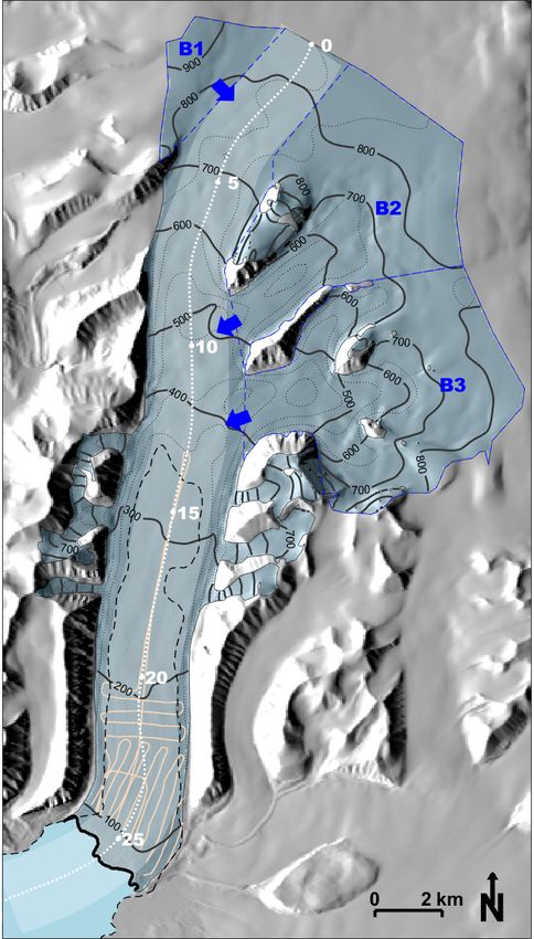
2116 J. Oerlemans et al.: Modelling of Tunabreen
Figure 1. Left: location of Tunabreen and Von Postbreen in Svalbard (inset). Background image is from a 2020 Sentinel-2 mosaic (https://
toposvalbard.npolar.no, last access: 24 May 2022). Right: photograph of Tunabreen in 2015 (© Anders Skoglund, Norwegian Polar Institute).
(Sevestre et al., 2018). Altogether, Tunabreen appears to be a ployed here is similar to the one used in a study of Monaco-
fairly representative glacier, albeit with a relatively high and breen in northern Spitsbergen (Oerlemans, 2018).
increasing surge frequency. To our knowledge a quantitative model has never been
Apart from the length fluctuations related to the surges, constructed for Tunabreen. We consider our study as a first
over the past 100 years Tunabreen has become shorter by step, with the focus on the integrated mass budget dynam-
about 1.5 km. This is likely due to an increasing equilibrium ics rather than ice mechanical processes. It is obvious that
line altitude (ELA) caused by rising air temperature (Førland MGMs cannot simulate more subtle processes like the sea-
et al., 2011), perhaps in combination with larger calving rates sonal cycle of the calving flux or the effect of high-water
associated with higher ocean temperature (Luckman et al., input (melt or rain) on sliding velocities. However, we be-
2015). lieve that MGMs are able to provide first-order estimates of
Before 1920 the lower parts of Tunabreen and of Von Post- the relation between glacier size and climatic regime.
breen were joined to form one front in the Tempelfjorden.
Length data back to 1870 exist (Flink et al., 2015) but are
not considered here for model validation because the focus is 2 Glacier model
on the period that Tunabreen was an independently calving
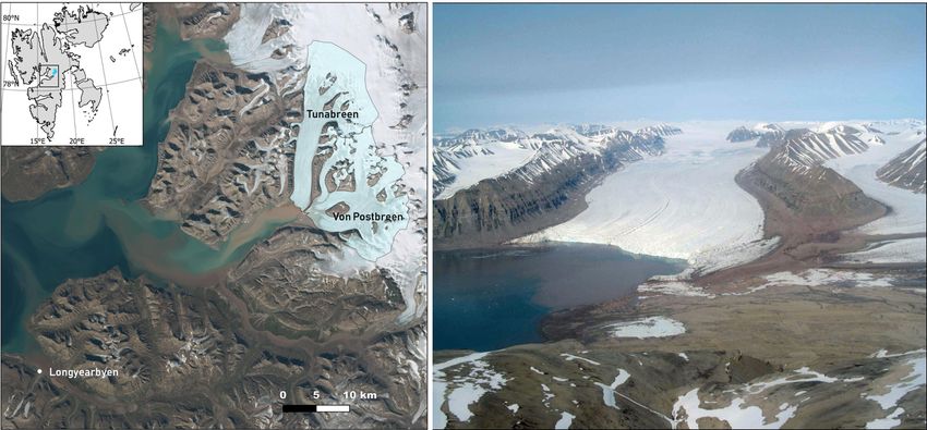
glacier. Tunabreen is modelled as a stream (flow band) of length L
The goal of this study is to analyse the mass budget of and constant width W . Three tributary glaciers and basins
Tunabreen, to determine how sensitive the glacier is to ongo- supply mass to the main stream if they have a positive mass
ing and future climate warming, and to see if the frequent budget (Fig. 3). A few minor tributaries are neglected be-
surging has an effect on its long-term retreat. The model cause they have no significant effect on the total mass budget
we used is a so-called minimal glacier model (MGM; Oer- of Tunabreen. The x axis, originating at the ice divide, fol-
lemans, 2011), in which dynamic processes are parameter- lows the centreline of the flow band. L is measured along this
ized. In this class of models, ice mechanics are not explicitly axis. Defined in this way, the glacier stand in 2009 serves as a
considered, but a number of essential feedback mechanisms reference point, with L = 25.8 km. The average width of the
can be dealt with (height–mass-balance feedback, effect of flow band is taken as 2200 m.
reversed bed slopes, variable calving rates, effect of regular Conservation of mass (or volume, since ice density is
surging on the long-term mass budget, inclusion of tributary considered to be constant) determines the evolution of the
glaciers and basins). The basic idea behind MGMs is that, glacier. It can be formulated as
with respect to long-term evolution of glaciers, ice mechan-
3
ics are “slaved” by the exchange of mass with the environ- dV X
ment (atmosphere and ocean). However, the most important = F + Mm + Mi = Mtot . (1)
dt i=1
mechanical effect, namely that glaciers are thicker when they
are longer and/or rest on a bed with a smaller slope, should Here V is the volume of the main stream of Tunabreen, F is
always be accounted for. We note that the model version em- the volumetric calving flux (< 0), M is the volumetric surface
The Cryosphere, 16, 2115–2126, 2022 https://doi.org/10.5194/tc-16-2115-2022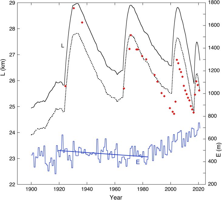
J. Oerlemans et al.: Modelling of Tunabreen                                                                                         2117

Figure 2. Length of Tunabreen from historical documents, aerial
photographs, and satellite images (Flink et al., 2015, with addi-
tions). The first four data points in red refer to the period that
Tunabreen and Von Postbreen formed a joined front.

mass budget of the main stream, and Mi represents the con-
tributions from the tributary glaciers. In the following sec-
tions a number of parameterizations are introduced concern-
ing the global ice mechanics, geometry, calving, and climate
forcing.
   We stress that a minimal glacier model is fundamentally
different from another class of approximate models that have
become popular, so-called lumped-parameter models (e.g.
Fowler et al., 2001; Benn et al., 2019). In the MGM the ba-
sic idea is to have a model description that deals with the
conservation laws integrated over an entire glacier. This is
essential if one wants to compute the evolution of a glacier         Figure 3. Map of Tunabreen. Surface contours (thick black lines) at
for imposed environmental change. In the lumped-parameter            100 m intervals are from the NPI S0 DEM (Norwegian Polar Insti-
model the focus is more on the details of local mechanical           tute, 2014), based on aerial photography from 2009 (lower glacier
processes and their interaction with hydrology and thermo-           tongue, 0–450 m a.s.l.) and 2011 (upper glacier, > 450 m a.s.l.). Bed
dynamics; the large-scale glacier parameters are then speci-         contours (dotted black lines) at 100 m intervals are based on the
fied.                                                                Fürst et al. (2018) reconstruction in the upper glacier and 2015
                                                                     helicopter radar (Katrin Lindbäck and Jack Kohler, in Welty et
                                                                     al., 2020) measurements (light-red lines) in the lower glacier. The
2.1   Prognostic equation for glacier length
                                                                     dashed subglacial contour shows the part of the bed below sea level.
                                                                     The centreline profile (dotted white line) along the 2200 m wide
The glacier volume V (of the main stream) is given by                main flow band (lighter blue) shows distance from the ice divide at
W LH̄ , where H̄ is the mean ice thickness. Differentiating          5 km intervals. The three upper basins (dashed blue outlines) supply
with respect to time yields                                          mass to the main flow band (blue arrows).


dV    d            dL    dH̄
   =W    LH̄ = W H̄    +L       = Mtot .                      (2)
dt    dt            dt     dt

https://doi.org/10.5194/tc-16-2115-2022                                                     The Cryosphere, 16, 2115–2126, 2022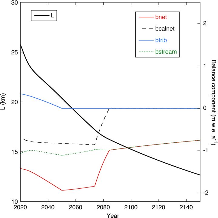
2118                                                                               J. Oerlemans et al.: Modelling of Tunabreen

The mean ice thickness is parameterized as (Oerlemans,
2011)
              α
H̄ = S(t)            L1/2 .                                   (3)
            1 + ν s̄
Here s̄ is the mean bed slope over the glacier length and
thus varies in time when the glacier length changes. S is the
“surge function”, making it possible to impose a surge (to be
discussed later). For a non-surging glacier we simply have
S(t) = 1. The parameter α can be interpreted as a measure
of the global basal resistance of the bed to ice flow and de-
termines the mean ice thickness for a given slope and glacier
length. Because of the abundant presence of soft and pre-
sumably mostly saturated sediments at the bed, the larger
glaciers on Svalbard experience rather low resistance and
therefore are comparatively thin (e.g. Benn and Evans, 2010).        Figure 4. Cross-section along centreline profile (shown in Fig. 3)
As shown later, the value of α is therefore relatively low (typ-     of the main flow band, with band averages of surface topography
ically ∼ 2 m1/2 as compared to a value of ∼ 3 m1/2 for many          (thin black line) from the 2009/2011 NPI DEM and bed topography
mid-latitude glaciers, or even ∼ 3.5 m1/2 for glaciers that are      from the Fürst et al. (2018) reconstruction (0–12.5 km), 2015 heli-
(partly) cold-based, like McCall glacier in Alaska (Oerle-           copter radar measurements (12.5–25 km), and hydrographic data in
mans, 2011)). The parameter ν determines the dependence              the fjord (Norwegian Mapping Authority Hydrographic Service). A
of the mean ice thickness on the mean bed slope. Based on            piecewise linear profile is fit to the bed profile for the MGM.
a large number of numerical experiments with an ice flow
model (Oerlemans, 2001), its dimensionless value was set to
10.                                                                  where b̄ is the mean bed elevation of the glacier (note that this
   Substituting the time derivative of Eq. (3) into Eq. (2) gives    quantity as well as H̄ depends on the glacier length, which
                                                                   in fact introduces the height–mass-balance feedback).
dV      W H̄     dS 3 dL
     =         L     + S        .                             (4)
 dt      S       dt    2 dt                                          2.2   Geometry
Rearranging then yields the prognostic equation for L:               The bed topography of the main stream as defined in Fig. 3
dL   2Mtot 2 1 dS                                                    is not very well known. The bed topography of Svalbard
   =      −       L.                                          (5)    glaciers has been modelled (Fürst et al., 2018) using a bal-
dt   3W H̄ 3 S dt
                                                                     ance velocity approach, overridden by observed topography
                                         ∂ s̄                        where radar data are available. For Tunabreen, radar sur-
We have neglected a term involving ∂L         because it is gener-
ally small. However, the dependence of the mean ice thick-           veys were carried out by the Norwegian Polar Institute over
ness on the mean bed slope is still retained through Eq. (3).        the lower part of the glacier (Fig. 3) so that the geome-
See Sect. 5 in Oerlemans (2011) for more discussion.                 try of this part of the bed is reasonably well constrained;
   The next step is to determine the mass budget, and we first       from ∼ 16 km and downglacier, the glacier bed is below
consider the surface budget. The balance rate is assumed to          sea level, typically −40 m. The details of the upper part of
be a linear function of altitude relative to the equilibrium line    the glacier bed are not dealt with; the smaller undulations
altitude E (see the compilation in Oerlemans and Van Pelt,           in this area presumably have a limited effect on the over-
2015):                                                               all dynamics of the glacier, and it is not clear how realistic
                                                                     all of the undulations really are. The bed undulations in the
ḃ = β(h − E),                                                (6)    lower part of the glacier have an amplitude of typically 10
                                                                     to 20 m, which is comparable to lateral (across-fjord) vari-
where β is the balance gradient, h is surface elevation, and E       ations as seen in the bathymetry in front of the glacier (see
is the equilibrium line altitude.                                    map at https://toposvalbard.npolar.no, last access: 5 Decem-
   The total mass loss or gain of the flow band is found by          ber 2021). In view of the flow band geometry adapted here,
integrating the balance rate over the glacier length:                the undulations are thus seen as irregularities with only a
            ZL                                                       local effect on the calving process. We also note that due
                                                                     to depositional and erosional processes the glacier bed may
Bs = βW          [H (x) + b (x) − E] dx
                                                                     be subject to significant changes even within a time span of
            0                                                        100 years. These considerations led to the choice of a simple

   = βW H̄ + b̄ − E L,                                        (7)    piecewise linear bed profile (red line in Fig. 4).

The Cryosphere, 16, 2115–2126, 2022                                                      https://doi.org/10.5194/tc-16-2115-2022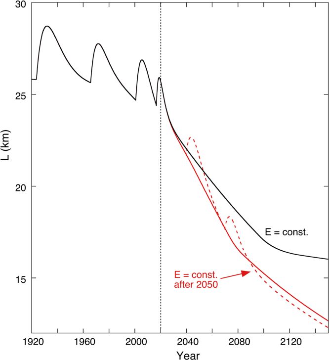
J. Oerlemans et al.: Modelling of Tunabreen                                                                                     2119

  Therefore we have                                                 model calving in detail have provided useful insights into the
                                                                    mechanical processes involved (e.g. Krug et al., 2014) but
b(x) = bh − s1 x       (0 ≤ x ≤ L1 ),                        (8)    cannot simply be adopted in a more general calving law for
b(x) = bd        (x > L1 ).                                  (9)    use in large-scale models of tidewater glaciers. Recent field
                                                                    and remote sensing studies show that an important control on
The bed profile thus drops off linearly, at a rate s1 , until x =   calving at many Svalbard tidewater glaciers is undercutting
L1 , from where the bed height has a constant value of bd . The     of the submerged ice front by melting (Petlicki et al., 2015;
parameters used here are bh = 650 m, s1 = 0.04, and bd =            Luckman et al., 2015; How et al., 2019). This implies that the
−40 m. It follows that L1 = 17 250 m.                               calving parameter depends on water temperature. However,
  The mean bed elevation b̄ and mean bed slope s̄ for given         since observations of water temperatures going further back
L are now easily found:                                             in time are not available, we use a constant value of c. By
                                                                    matching with the mean observed calving rate for the period
b̄ = {(bh − s1 L1 /2)L1 + bd (L − L1 )} /L     (L > L1 ), (10)      2012–2019 (namely 270 m a−1 ) and a typical water depth of
b̄ = (bh − s1 L/2)      (L ≤ L1 ),                          (11)    40 m, we find c = 6.75 a−1 . This may overestimate calving
s̄ = (bh − bd /L       (L > L1 ),                           (12)    rates further back in time because water temperatures were
                                                                    presumably lower in the 20th century. Unfortunately, it is not
s̄ = s1   (L ≤ L1 ).                                        (13)
                                                                    possible to give a quantitative evaluation of the uncertainty in
With these expressions the mean ice thickness as well as the        c for longer periods because data are not available. Also, we
surface mass budget of the main stream can be calculated for        could not find in the literature a study in which a systematic
any value of L.                                                     relation between calving rate and surging phase was found.
   In the present model, the tributary glaciers are just consid-       The thickness at the glacier front is not explicitly calcu-
ered to be buckets with a fixed geometry. When they have a          lated and therefore has to be parameterized. As for the stud-
positive budget they spill over and supply mass to the main         ies of Hansbreen and Monacobreen referred to above, the fol-
glacier. The model has no intention to describe the physical        lowing parameterization is used:
process of how the tributaries flow into the main stream. Al-
                                                                    Hf = max κ H̄ ; δ .                                        (16)
though in reality a tributary glacier with a negative mass bud-
get can for a short period still deliver some mass, this will al-   Here δ is the ratio of water density to ice density, and κ is
ways be a small amount during a limited period of time. The         a constant giving the ratio of the frontal ice thickness to the
mass budget of an individual basin is then given by                 mean ice thickness. For the current geometry of Tunabreen,
         ZZ                                                         κ∼= 0.3. So according to Eq. (13) the ice thickness can never
                                                                    be less than the critical thickness for flotation. For the simula-

Mi = β        (h − E) dA = βAi h̄i − E ,                    (14)
                                                                    tions discussed in this paper, flotation was never approached.
            Ai
                                                                    The use of Eqs. (12) and (13) allows a smooth transition be-
where Ai is the area, and h̄i is the mean surface elevation of      tween a land-terminating and tidewater glacier, a prerequisite
basin i (determined from a digital elevation model). When           for long-term simulations in which a model glacier should
Mi > 0, the mass is added to the budget of the main stream.         have the possibility of growing from zero volume to a long
When Mi ≤ 0, there is no coupling between basin and main            calving glacier and vice versa.
stream. For the present geometry of the basins this happens
                                                                    2.4   Imposing surges
when E > 853, 747, and 663 m a.s.l. for basins 1, 2, and 3,
respectively.                                                       In the MGM, surges are not internally generated but have
                                                                    to be prescribed. For a discussion on surging mechanisms
2.3   Calving rate
                                                                    the reader is referred to, among others, Sund et al. (2009),
As in earlier studies with MGMs (Hansbreen, Oerlemans et            Mansell et al. (2012), and Benn et al. (2019). Including
al., 2011; Monacobreen, Oerlemans, 2018), the calving rate          surges is potentially important because they affect the mass
is assumed to be proportional to the water depth d. The calv-       budget and thus may exert an influence on the long-term evo-
ing flux can then be formulated as                                  lution of a glacier. When a glacier surges, and its front ad-
                                                                    vances, the mean surface elevation decreases, and the abla-
F = −c d W Hf .                                             (15)    tion zone expands. In the MGM a surge is imposed through
                                                                    the function S(t) in Eq. (3). A fast decrease in S implies
Here Hf is the ice thickness at the glacier front, and c is the     a smaller ice thickness, and to fulfil mass conservation the
“calving parameter”. The dependence of the calving flux on          glacier length has to increase. So the surge is in fact modelled
water depth has been suggested by, among others, Brown et           as a sudden reduction in the mean basal resistance without
al. (1982), Funk and Röthlisberger (1989), Pelto and War-           specifying its cause, where it is initiated, or how it propa-
ren (1991), and Björnsson et al. (2000). Recent attempts to         gates.

https://doi.org/10.5194/tc-16-2115-2022                                                   The Cryosphere, 16, 2115–2126, 2022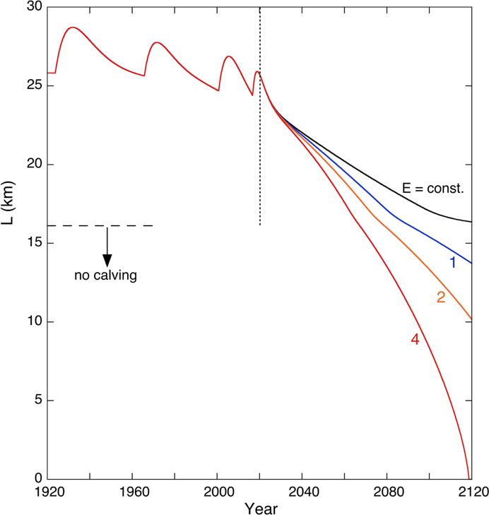
2120                                                                           J. Oerlemans et al.: Modelling of Tunabreen

  In the model the surge function is prescribed as (Oerle-       shape is superposed and centred around the year 1975 and
mans, 2011)                                                      has a characteristic window of 30 years. In the simulation
                                                                 of the observed length record, the parameters E0 , c1 , and c2
S (t) = 1 − S0 (t − t0 )e−(t−t0 )/ts .                   (17)
                                                                 are determined in such a way that the best possible match
The surge starts at t = t0 ; two additional parameters, S0 and   between observed and simulated glacier length is obtained.
ts , determine the amplitude and the characteristic timescale    So in effect, the climate forcing is reconstructed by inverse
of the surge. In the earlier studies of Abrahamsenbreen and      modelling on the glacier length observations.
Monacobreen, periodic surging was imposed, with fixed val-
ues of S0 and ts according to the observed single surge
of these glaciers. However, in the case of Tunabreen four
surges of different amplitude and duration have been ob-         3   Basic experiments on the sensitivity of Tunabreen to
served, which are included in the model by using different           climate change
surge parameters. This allows a closer match between ob-
served and simulated glacier length.                             Before discussing simulations with the time-dependent cli-
                                                                 matic forcing described in Sect. 2.5, it is useful to obtain a
2.5    Climate forcing                                           feeling for the sensitivity of glacier length to environmental
                                                                 parameters like the ELA and the calving rate. We can obtain
Information on the climate history of Svalbard is mainly         insight into climate sensitivity and response times by doing
based on geomorphological and geological studies (e.g.           this in numerical experiments with stepwise forcing imposed
CAPE, 2006; Axford et al., 2017; Farnsworth et al., 2020).       on a steady state.
The general picture emerging from these studies is that of          First of all the value of α in Eq. (3) was obtained by
a warmer mid-Holocene climate with much reduced glacier          matching the simulated and observed mean ice thickness (for
extent over Svalbard, with gradual cooling afterwards. This      the profile shown in Fig. 4), yielding α = 1.96 m1/2 . With
cooling of 1 to 3 ◦ C is normally interpreted as a direct in-    E = 524 m a.s.l. and c = 6.75 a−1 , the model now produces
solation effect (changing orbital parameters reducing sum-       a steady-state glacier with a length that corresponds to the
mer radiation). Most glaciers on Svalbard reached maximum        situation around 1920 (L ≈ 25.8 km). In this case the net bal-
stands during the local Little Ice Age, between 1850 and         ance of the main stream is −0.33 m w.e. a−1 , of the tributaries
1900 (e.g. Martin-Moreno et al., 2017). Significant warm-        1.10 m w.e. a−1 , and from calving −0.76 m w.e. a−1 , the lat-
ing started around 1900 (Divine et al., 2011) and contin-        ter obtained by dividing calving flux by glacier area for a
ues until today, but with some interruptions, notably between    good comparison. So although the main stream also has an
1950 and 1980. On Svalbard the relation between the ELA          accumulation area (Fig. 3), its mean surface balance is neg-
and meteorological parameters is perhaps more complicated        ative, and the influx from the tributaries is essential to main-
than for mid-latitude conditions, partly because refreezing      tain the long glacier tongue of Tunabreen.
plays a larger role. We have considered results from a de-          In Fig. 5 glacier length is shown for different perturbations
tailed energy-balance model of Svalbard mass balance (van        of the ELA. All integrations start at t = 0, and the pertur-
Pelt et al., 2019) to derive model ELA values for Tunabreen      bation in the forcing is applied at t = 1500 a (to make sure
for the period 1957–2020. However, to have a useful ELA          that the initial state represents a steady state). For a 25 m
history to simulate observed glacier length, this reconstruc-    rise in the equilibrium line the glacier would become about
tion has to be extended backwards to at least 1900. We tried     5 km shorter, but it takes a long time to approach a steady
to do this by means of a reduced major axis regression on        state (∼ 400 years). The large climate sensitivity (defined as
the modelled ELA to meteorological parameters observed at        ∂L/∂E) and long timescale are a consequence of the very
Longyearbyen (Nordli et al., 2020; Førland et al., 2011, with    small mean bed (and surface) slope (Oerlemans, 2001, 2011).
updates). The correlation with summer temperature appears        For larger perturbations of the ELA (+50 m, +100 m) the
to be significant (coefficient 0.46) but in the end explains     sensitivity becomes less and the response time shorter (typi-
only 25 % of the ELA variability. In spite of this, we recon-    cally ∼ 100 years for the case with 1E = +100 m). This is
structed the ELA history back to 1900 (referred to later as      related to the position of the glacier snout. When the glacier
ELALYR ). Some test calculations with the resulting forcing      snout is still calving but on the upward-sloping part of the
function were not satisfactory (this is shown and discussed      bed (Fig. 4), the dependence of the calving flux on the water
later), and therefore we decided to use for the reference ex-    depth makes the glacier more stable (a smaller change in L is
periment a forcing function of a smooth and simple form.         needed to achieve the necessary change in the mass budget to
The forcing is written as                                        acquire a new equilibrium state). The height–mass-balance
                                                2                feedback becomes particularly effective for negative values
E (t) = E0 + c1 (t − 1900)2 − c2 e−((t−1975)/30) .       (18)
                                                                 of 1E. Because the calving rate is constant, due to constant
According to Eq. (15), the equilibrium line rises quadrati-      water depth, there is no way for the model glacier to stabi-
cally in time. On this rise a minor depression of Gaussian       lize. In reality, the advance would come to a halt because the

The Cryosphere, 16, 2115–2126, 2022                                                 https://doi.org/10.5194/tc-16-2115-2022
J. Oerlemans et al.: Modelling of Tunabreen 2121
Figure 6. Glacier length L for a very slowly increasing ELA (E).
Three regimes are identified (I, II, III) for which the sensitivity of
glacier length to the ELA (∂L/∂E) differs significantly.
Figure 5. Evolution of glacier length for different perturbations of
the ELA (1E) and different values of the calving parameter c.
in a climate sensitivity comparable to that for regime I (now
∂L/∂E ≈ 140). This calculation thus illustrates once more
glacier front would eventually encounter deeper water and how important geometric factors are when considering the
higher water temperatures. response of individual glaciers to climate change.
The red curves in Fig. 5 show the response of the glacier to
changes in the calving parameter c. For a 50 % larger calving
parameter, the response of the glacier is comparable to that 4 Simulating the evolution of Tunabreen during the
for a 35 m increase in the ELA. For a 25 % decrease in the past 100 years
calving rate, the glacier grows slowly but steadily. The appar-
ent differences in the sensitivity for smaller and larger pertur- We now turn to simulation of the observed length record. The
bations of the ELA call for a further numerical experiment in best possible result for optimal values of the surge parame-
which this is explored. One way to approach this is to do a ters (t0 , S0 , ts ) and climatic parameters (E0 , c1 , c2 ) is shown
long integration with very “slow” forcing (here slow means in Fig. 7. The value of E0 was set to a value that makes
that the glacier is always close to an equilibrium state). Fig- the simulated glacier length in 1924 equal to the observed
ure 6 shows the result of an integration in which the ELA in- value (E0 = 490 m a.s.l.). The surge amplitudes have been
creases at a rate of 0.05 m a−1 . Evidently, with respect to the chosen such that the advance during the surge approximately
climate sensitivity ∂L/∂E (a dimensionless quantity), three matches the observed length change.
regimes can be distinguished. In regime I the glacier front During the 1924 surge, which has the largest ampli-
is calving and located on the part of the bed with constant tude (1L ≈ 3 km), the associated maximum reduction in the
water depth. The mean climate sensitivity in this regime is mean ice thickness (and surface elevation) is about 25 m.
∂L/∂E ≈ 150. As noted before, this very large value is a di- Although the calving rate is constant, the calving flux de-
rect consequence of the small mean bed slope (strong height– creases slightly because the frontal ice thickness is somewhat
mass-balance feedback). In regime II the glacier front is on smaller. Altogether, at the end of the surge the net mass bud-
the part of the bed where the water depth decreases when go- get perturbation of the main stream is about −0.24 m w.e. a−1
ing inland. When the glacier becomes shorter to adapt to the and of the entire glacier about −0.18 m w.e. a−1 . It should
increasing ELA, the calving rate decreases strongly (accord- be noted that there are two effects leading to a negative bal-
ing to Eq. 12). A very small change in L is therefore suf- ance perturbation: (i) the lowering of the glacier surface and
ficient to restore equilibrium, and consequently the climate (ii) the extension of the ablation zone. Together with the cli-
sensitivity is small (∂L/∂E ≈ 15). In regime III the glacier matic forcing this affects the retreat of the glacier front after
has become a land-terminating glacier. The combined effect the surge.
of a larger mean bed slope and the absence of calving results
https://doi.org/10.5194/tc-16-2115-2022 The Cryosphere, 16, 2115–2126, 20222122 J. Oerlemans et al.: Modelling of Tunabreen
Figure 7. Simulation of glacier length L achieved after optimiza- Figure 8. Simulation of glacier length L with ELALYR as climate
tion of the model parameters. Observations are indicated by red forcing (scale at right). Observations are indicated by red dots. The
dots. The blue line shows the optimal ELA forcing (scale at right). simulation shown by the solid line is tuned to the first observed
Glacier length simulated for a case without surging is shown by the glacier length (1926); the dotted line is tuned to the last observed
dotted line. glacier length (2020).
For the 1966–1971 surge the simulated retreat is some- 2010 (Geyman et al., 2022). The DEMs allow an indepen-
what too fast. However, increasing the surge parameter ts dent check on the model performance. The mean change in
does not help because it leads to a glacier length that is too surface elevation for Tunabreen over the period 1936–2010,
large when the next surge starts. The last surge comes fast based on gridded DEM data, amounts to −0.30 m w.e. a−1 .
and has a small amplitude, but it was possible to choose the The mean net balance calculated for this period from the
surge parameters in such a way that the 2020 observed length model output (run of Fig. 7) is −0.25 m w.e. a−1 . We thus
is reproduced. The dotted line in Fig. 7 shows the result for conclude that the calibrated model result is in broad agree-
a run without surging. In this case the glacier length stays ment with the geodetic evidence.
close to the minimum values after each surge except for the At this point it is interesting to return to the ELA
last surge. The 2016 surge comes so fast after the previous reconstruction based on energy-balance modelling and
surge that the glacier has no time to adjust its length to the the Longyearbyen meteorological record as discussed in
higher ELA. This is reflected in the difference between the Sect. 2.5 (ELALYR ). In Fig. 8 computed glacier length is
change in length over the past 100 years (≈ 2 %) as com- shown for the ELALYR forcing. Two simulations are shown:
pared to the change in volume (≈ 11 %). The decrease in one in which the first data point (1926) is matched with the
mean glacier length has thus been limited due to the increas- observed length, one in which the last data point (2020) is
ing surge frequency, at the cost of a reduction in the mean matched. The corresponding values of E0 are 528 and 533 m.
ice thickness. The result of Fig. 7 has been obtained with the None of the simulations are good, and adjusting the surge pa-
following parameters of the ELA history: E0 = 524 m a.s.l., rameters does not give an improvement. The reason for the
c1 = 0.0095 m a−2 , c2 = 40 m. Changing these parameters discrepancy between observed and simulated glacier length
leads to a larger difference between observed and simulated is the small but significant decline in the ELA during the
glacier length. This cannot be compensated by adjusting the period 1920–1980. When the equilibrium line starts to rise
surge parameters; i.e. the parameter sets (t0 , S0 , ts ) and (E0 , around 1985, the response of the glacier is too slow to catch
c1 , c2 ) play fairly independent roles in the model. The ELA up with the observed retreat over the last 100 years. It thus
history that delivers the best simulation is therefore well de- appears that the value of ELALYR as a climate proxy for
termined and reveals that a 135 m increase in the ELA over Tunabreen is limited.
the past 50 years is sufficient to explain the behaviour of The mass-balance simulation with a regional climate
Tunabreen. model by van Pelt et al. (2019) yields a mean increase of
Two digital elevation models (DEMs) for Svalbard have 4.6 m a−1 of the ELA over the period 1957–2018. This is
recently been published, referring to the years 1936 and substantially larger than the 3.2 m a−1 found for the recon-
The Cryosphere, 16, 2115–2126, 2022 https://doi.org/10.5194/tc-16-2115-2022J. Oerlemans et al.: Modelling of Tunabreen 2123
structed forcing. The discrepancy is substantial and hard
to explain. However, since the simulation by van Pelt et
al. (2019) does not go further back in time than 1957, a thor-
ough comparison remains difficult.
Referring to the sensitivity of the glacier length to the calv-
ing parameter (Fig. 5), it is obvious that the use of a fixed
calving parameter is a limitation of the calibration procedure.
It would even be possible to keep the ELA fixed and vary c.
Possibly variations in c and the ELA work in parallel be-
cause both quantities presumably increase with atmospheric
temperature (assuming that water temperature in summer is
related to air temperature). However, increasing c would im-
ply a smaller increase in the ELA, and the discrepancy be-
tween the reconstructed ELA history and the simulation by
van Pelt et al. (2019) would become larger.
5 The future evolution of Tunabreen
Having calibrated the model with observations over the past
100 years, we now consider future climate change scenar-
ios and see how Tunabreen might change in the coming 100
years. Rather than applying the output from regional climate
model simulations with all their uncertainties, we prefer a Figure 9. Glacier length L for different climate change experi-
ments. The black curve refers to a calculation in which E is kept
simple approach in which the equilibrium line rises at a con-
constant at its 2000–2019 mean value. The colour labels refer to the
stant rate after the year 2020.
imposed constant rate of change in E per year from 2020 onwards.
In Fig. 9 some results of climate change experiments for
the next 100 years are summarized. In the reference run
the ELA is kept constant at the 2020 value from the recon-
struction, namely 656 m a.s.l. In this case the model glacier
In Fig. 10 a calculation is shown for an optimistic cli-
retreats during the next 100 years at an almost linear rate
mate change scenario, in which the equilibrium line rises by
of ∼ 80 m a−1 , which illustrates by how much the current
2 m a−1 until the year 2050 and remains constant afterwards
glacier stand is out of equilibrium with the present climate.
(we refer to this calculation as the “Paris run”). We show the
After the year 2110 the retreat slows down, and the glacier
result until the year 2150 to see if by this time the glacier
approaches a new steady state with a length of about 16 km
would have reached a new steady state. Obviously, this is not
and no calving anymore.
the case, although the rate of retreat slows down. This case
For the intermediate climate warming scenario (the equi-
clearly illustrates that it takes a long time before limiting cli-
librium line then rises by 2 m a−1 ), Tunabreen would re-
mate warming has a significant effect on the retreat of large
treat by about 15 km over the next 100 years. During the
glaciers.
retreat the net balance would steadily decrease to about
The dashed curve in Fig. 10 represents the result for the
−2.0 m w.e. a−1 ; i.e. the glacier is getting more and more out
Paris run with two surges imposed, initiated at the years 2040
of balance. In the year 2026 basin 3 would no longer deliver
and 2070. The choice of those years is quite arbitrary of
mass to the main stream; for basin 2 this happens in the year
course, but it serves to demonstrate that surges do not seem
2063.
to have an impact on the long-term evolution of the glacier.
For the case of a 4 m a−1 rise in the equilibrium line, the
To further illustrate the interaction between climate
retreat is obviously much stronger, and by the year 2120
change and the mass budget of Tunabreen, we show in
Tunabreen has almost disappeared. In the year 2081, E =
Fig. 11 the various mass balance components as a function of
900 m a.s.l., and virtually the entire glacier is below the equi-
time for the Paris run (without additional surges). All terms
librium line.
in the mass budget equation have been converted to specific
It can be seen in all the simulations that the retreat slows
balance rate for an easy comparison; e.g. the calving flux has
down when the length becomes less than 17.2 km, i.e. at the
been divided by the glacier area. First of all, as noted before,
point where the modelled bed elevation starts to increase
the balance of the main stream (bstream) is always negative,
from −40 m to sea level (at x = 16.2 km); see Fig. 9. This
and the glacier lives on the contributions from the tributaries
is in line with the result of Fig. 6.
(btrib). After 2048 the specific contribution from the tribu-
taries becomes zero, and the model glacier is basically a body
https://doi.org/10.5194/tc-16-2115-2022 The Cryosphere, 16, 2115–2126, 20222124 J. Oerlemans et al.: Modelling of Tunabreen
Figure 11. Glacier length (solid black line, scale at left) and mass
balance components (scale at right) for the “Paris run”.
Figure 10. Glacier length L for the “Paris run” (constant ELA af-
ter 2050), shown in red. The black curve refers to the calculation
in which E is kept constant at its 2020 reconstructed value (as in get the calving and surging to occur at the right place and
Fig. 9). The dashed curve represents the Paris run with two surges time!
imposed, starting in 2040 and 2070. As has been found for other larger glaciers in Svalbard,
Tunabreen appears to be very sensitive to climate change.
The common factor is the small surface slope, also when con-
of ice melting away. After 2073 the calving starts to decrease, sidered in a global perspective. From a purely geometric ar-
and by 2084 it has become zero. gument, ∂L/∂E ∼ −2/s̄ (Oerlemans, 2001). The mean slope
of Tunabreen is 0.031, comparable to that of many other
glaciers in Svalbard like, for example, Monacobreen (0.025),
6 Discussion Kongsvegen (0.032), and Kronebreen (0.025). A characteris-
tic value of ∂L/∂E therefore is −65; i.e. a 100 m rise in the
Tunabreen is a special glacier because of its complex surg- equilibrium line implies a glacier retreat over 6.5 km (when
ing behaviour, which poses a real challenge for a modelling a steady state would be reached). For larger mid-latitude
study. The MGM, based on the view that the evolution of mountain glaciers values of ∂L/∂E are in the range of −10
a glacier is primarily determined by the exchange of mass to −30, while for long glaciers in Alaska and Patagonia they
with its surroundings, offers a relatively simple tool to study are typically in the range of −30 to −60. Although other
the response of Tunabreen to changing environmental condi- factors than mean slope play a role, it is fair to conclude
tions. The application is straightforward and requires as ge- that the larger glaciers on Svalbard are the most sensitive
ometric input only a topographic map and a schematic bed in the world. This is in line with the idea that during the
profile along the main flow band. We are aware of the limi- mid-Holocene Climatic Optimum the degree of glacieriza-
tations inherent to a simple modelling approach as employed tion in Svalbard was considerably smaller than today (e.g.
here. The dynamic interaction between the tributaries and the Fjeldskaar et al., 2017).
main stream is not explicitly described, and the calving pro- Our numerical experiments suggest that typical fluctua-
cess is formulated in a simple way. Since there is no spatial tions in calving rates and equilibrium line altitudes have
resolution, subtle effects associated with undulations in the comparable effects on the evolution of Tunabreen. A 50 %
bed cannot occur. Therefore, in the end one would like to increase in the calving rate has the same effect as a 35 m
repeat the simulations presented here with a comprehensive increase in the ELA (Fig. 6). It is conceivable that in a
glacier flow model with full spatial resolution. However, it warming climate with increasing ocean temperatures, calv-
will not be an easy task to prepare the necessary input fields, ing rates will become larger. This implies that the glacier re-
formulate boundary conditions in a straightforward way, and treat curves shown in Fig. 9 represent conservative estimates.
The Cryosphere, 16, 2115–2126, 2022 https://doi.org/10.5194/tc-16-2115-2022J. Oerlemans et al.: Modelling of Tunabreen 2125
However, further studies on the relation between ocean tem- References
peratures and calving rates on a multi-annual timescale are
needed to make a meaningful estimate of how calving might Axford, Y., Levy, L. B., Kelly, M. A., Francis, D. R., Hall, B. L.,
enhance the retreat of Tunabreen in the near future. Langdon, P. G., and Lowell, T. V.: Timing and magnitude of early
to middle Holocene warming in East Greenland inferred from
We did not find a significant impact of surging on the
chironmids, Boreas, 46, 678–687, 10.1111/bor.12247, 2017.
evolution of Tunabreen. Although a surge initiates a nega- Benn, D. I. and Evans, D. J. A.: Glaciers & Glaciation, Hodder Ed-
tive perturbation of the mass budget for some years and re- ucation (London), 802 pp., ISBN: 978 0 340 905791, 2010.
duces the glacier volume slightly, this apparently has no last- Benn, D. I., Fowler, A. C., Hewitt, I., and Sevestre, H.: A
ing effect. The same conclusion was reached in earlier stud- general theory of glacier surges, J. Glaciol., 65, 701–716,
ies of Abrahamsenbreen (Oerlemans and van Pelt, 2015) and https://doi.org/10.1017/jog.2019.62, 2019.
Monacobreen (Oerlemans, 2018), and it probably applies to Björnsson, H., Pálsson, F., and Gudmundsson, S.: Jökulsárlón at
most long glaciers on Svalbard. However, with respect to ice Breidamerkursandur, Vatnajökull, Iceland: 20th century changes
caps that have surging parts (like Austfonna), the situation and future outlook, Jökull, 50, 1–18, 2000.
may be different. Błaszczyk, M., Jania, J., and Hagen, J. O.: Tidewater Glaciers of
Svalbard: Recent changes and estimates of calving fluxes, Polish
Polar Res., 30, 85–142, 2009.
Brown, C. S., Meier, M. F., and Post, A.: Calving speed of Alaska
Code availability. The code is available on request from Johannes
tidewater glaciers with applications to the Columbia Glacier,
Oerlemans.
Alaska, U. S. Geol. Surv. Prof. Pap. 1258-C, 13 pp., 1982.
CAPE-Last Interglacial Project Members: Last Interglacial
Arctic warmth confirms polar amplification of cli-
Data availability. Data on glacier length (Fig. 2) were compiled mate change, Quaternary Sci. Rev., 25, 1383–1400,
from various sources and can be obtained from Johannes Oerle- https://doi.org/10.1016/j.quascirev.2006.01.033, 2006.
mans. Meteorological data is described by Førland et al. (2011) and Divine, D., Isaksson, E., Martma, T., Meijer, H. A. J., Moore, J.,
accessible at https://www.met.no/en/free-meteorological-data (last Pohjola, V., Van de Wal, R. S. W., and Godtliebsen, F.: Thousand
access: 31 May 2022). For radar data on bed topography inquiries years of winter surface air temperature variations in Svalbard and
can be made with Jack Kohler. northern Norway reconstructed from ice- core data, Polar Res.,
30, 7379, https://doi.org/10.3402/polar.v30i0.7379, 2011
Farnsworth, W. R., Allaart, L., Ingólfsson, Ó., Alexander-
Author contributions. JO developed the model code and performed son, H., Forwick, M., Noormets, R., Retelle, M., and
the simulations. JK analysed and evaluated data on bedrock topog- Schomacker, A.: Holocene glacial history of Svalbard: Sta-
raphy and glacier length. AL derived and compiled data on calving tus, perspectives and challenges, Earth-Sci. Rev., 208, 1–28,
rates. JO prepared the manuscript with contributions from all co- https://doi.org/10.1016/j.earscirev.2020.103249, 2020.
authors. Fjeldskaar, W., Bondevik, S., and Amantov, A.:
Glaciers on Svalbard survived the Holocene ther-
mal optimum, Quaternary Sci. Rev., 119, 18–29,
Competing interests. The contact author has declared that neither https://doi.org/10.1016/j.quascirev.2018.09.003, 2017.
they nor their co-authors have any competing interests. Flink, A. E., Noormets, R., Kirchner, N., Benn, D. I.,
and Lovell, H.: The evolution of a submarine landform
record following recent and multiple surges of Tunabreen
Disclaimer. Publisher’s note: Copernicus Publications remains glacier, Svalbard, Quaternary Sci. Rev., 108, 37–50,
neutral with regard to jurisdictional claims in published maps and https://doi.org/10.1016/j.quascirev.2014.11.006, 2015.
institutional affiliations. Førland, E. J., Benestad, R., Hanssen-Baur, I., Haugen, J. E.,
and Skaugen, T. E.: Temperature and precipitation develop-
ment at Svalbard 1900–2100, Adv. Meteorol., 2011, 893790,
Acknowledgements. We are grateful to Francisco Navarro and an https://doi.org/10.1155/2011/893790, 2011.
anonymous referee for their detailed reviews that helped to improve Fowler, A. C., Murray, T., and Ng, F. S. L.: Thermally controlled
this paper. glacier surges, J. Glaciol., 47, 527–538, 2001.
Funk, M. and Röthlisberger, H.: Forecasting the effects of a planned
reservoir which will partially flood the tongue of Unteraar-
gletscher in Switzerland, Ann. Glaciol., 13, 76–81, 1989.
Review statement. This paper was edited by Carlos Martin and re-
Fürst, J. J., Navarro, F., Gillet-Chaulet, F., Huss, M., Moholdt,
viewed by Francisco Navarro and one anonymous referee.
G., Fettweis, X., Lang, C., Seehaus, T., Ai, S., Benham, T. J.,
Benn, D. I., Björnsson, H., Dowdeswell, J. A., Gabriec, M.,
Kohler, J., Lavrentiev, I., Lindbäck, K., Melvold, K., Pettersson,
R., Rippin, D., Saintenoy, A., Sánchez-Gámez, P. Sculer, T. V.,
Sevestre, H., Vasilenko E., and Braun, M. H.: The ice free to-
pography of Svalbard, Geophys. Res. Lett., 45, 11760–11769,
https://doi.org/10.1029/2018GL079734, 2018.
https://doi.org/10.5194/tc-16-2115-2022 The Cryosphere, 16, 2115–2126, 20222126 J. Oerlemans et al.: Modelling of Tunabreen Geyman, E. C., Van Pelt, W. J. J., Maloof, A. C., Faste Aas, Oerlemans, J.: Minimal Glacier Models, 2nd Edn., Igitur, Utrecht H., and Kohler, J.: Historical glacier change on Svalbard pre- University, ISBN 978-90-6701-022-1, 2011. dicts doubling of mass loss by 2100, Nature, 601, 374–379, Oerlemans, J.: Modelling the late Holocene and future evolution of https://doi.org/10.1038/s41586-021-04314-4, 2022. Monacobreen, northern Spitsbergen, The Cryosphere, 12, 3001– How, P., Schild, K. M., Benn, D. I., Noormets, R., Kirchner, N., 3015, https://doi.org/10.5194/tc-12-3001-2018, 2018. Luckman, A., Vallot, D., Hulton, N. R., and Borstad, C.: Calv- Oerlemans, J. and van Pelt, W. J. J.: A model study of Abrahamsen- ing controlled by melt-under-cutting: detailed calving styles re- breen, a surging glacier in northern Spitsbergen, The Cryosphere, vealed through time-lapse observations, Ann. Glaciol., 60, 20– 9, 767–779, https://doi.org/10.5194/tc-9-767-2015, 2015. 31, https://doi.org/10.1017/aog.2018.28, 2019. Pelto, M. S. and Warren, C. R.: Relationship between tidewater Krug, J., Weiss, J., Gagliardini, O., and Durand, G.: Combin- glacier calving velocity and water depth at the calving front, Ann. ing damage and fracture mechanics to model calving, The Glaciol., 15, 115–118, 1991. Cryosphere, 8, 2101–2117, https://doi.org/10.5194/tc-8-2101- Petlicki, M., Cieply, M., Jania, J. A., Prominska, A., Kin- 2014, 2014. nard, C.: Calving of a tidewater glacier driven by Lefauconnier, B. and Hagen, J.O.: Surging and calving glaciers melting at the waterline, J. Glaciol., 61, 851–863, in eastern Svalbard, Nor. Polarinst. Medd., 116, 130 pp., ISBN https://doi.org/10.3189/2015JoG15J062, 2015. 8290307942 9788290307948, 1991. Sevestre, H., Benn D. I., Luckman, A., Nuth, C., Kohler, J. Lind- Luckman, E., Benn, D. I., Cottier, F., Bevan, S., Nilsen, bäck, K., and Pettersson, R.: Tidewater glacier surges initi- F., and Inall, N.: Calving rates at tidewater glaciers vary ated at the terminus, J. Geophys. Res.-Earth, 123, 1035–1051, strongly with ocean temperature, Nat. Commun., 6, 1–7, https://doi.org/10.1029/2017JF004358, 2018. https://doi.org/10.1038/ncomms9566, 2015. Sund, M., Eiken, T., Hagen, J. O., and Kääb, A.: Svalbard surge dy- Mansell, D., Luckman, A., and Murray, T.: Dynamics of tidewater namics derived from geometric changes, Ann. Glaciol., 50, 50– surge-type glaciers in northwest Svalbard, J. Glaciol., 58, 110– 61, 2009. 118, https://doi.org/10.3189/2012JoG11J058, 2012. van Pelt, W., Pohjola, V., Pettersson, R., Marchenko, S., Kohler, Martín-Moreno, A., Alvarez, F. A., and Hagen J. O.: “Lit- J., Luks, B., Hagen, J. O., Schuler, T. V., Dunse, T., Noël, tle Ice Age” glacier extent and subsequent retreat B., and Reijmer, C.: A long-term dataset of climatic mass bal- in Svalbard archipelago, Holocene, 27, 1379–1390, ance, snow conditions, and runoff in Svalbard (1957–2018), The https://doi.org/10.1177/0959683617693904, 2017. Cryosphere, 13, 2259–2280, https://doi.org/10.5194/tc-13-2259- Nordli, Ø., Wyszyński, P., Gjelten, H. M., Isaksen, K., Łupikasza, 2019, 2019. E., Niedźwiedź, T., and Przybylak, R.: Revisiting the extended Welty, E., Zemp, M., Navarro, F., Huss, M., Fürst, J. J., Gärtner- Svalbard Airport monthly temperature series, and the com- Roer, I., Landmann, J., Machguth, H., Naegeli, K., An- piled corresponding daily series 1898–2018, Polar Res., 39, dreassen, L. M., Farinotti, D., Li, H., and GlaThiDa Con- https://doi.org/10.33265/polar.v39.3614, 2020. tributors: Worldwide version-controlled database of glacier Norwegian Polar Institute: Terrengmodell Svalbard (S0 thickness observations, Earth Syst. Sci. Data, 12, 3039–3055, Terrengmodell), Norwegian Polar Institute [data set], https://doi.org/10.5194/essd-12-3039-2020, 2020. https://doi.org/10.21334/npolar.2014.dce53a47, 2014. Oerlemans, J.: Glaciers and Climate Change, A.A. Balkema Pub- lishers, 148 pp., ISBN 9026518137, 2001. The Cryosphere, 16, 2115–2126, 2022 https://doi.org/10.5194/tc-16-2115-2022
You can also read