Mandatory Retention Rules and Bank Risk - by Yuteng Cheng
←
→
Page content transcription
If your browser does not render page correctly, please read the page content below
Staff Working Paper/Document de travail du personnel—2023-3
Last updated: August 9, 2023

Mandatory Retention Rules
and Bank Risk
by Yuteng Cheng

Banking and Payments Department
Bank of Canada
ycheng@bankofcanada.ca

Bank of Canada staff working papers provide a forum for staff to publish work-in-progress research independently
from the Bank’s Governing Council. This research may support or challenge prevailing policy orthodoxy. Therefore,
the views expressed in this paper are solely those of the authors and may differ from official Bank of Canada views.
No responsibility for them should be attributed to the Bank.

DOI: https://doi.org/10.34989/swp-2023-3 | ISSN 1701- 9397                                   ©2023 Bank of Canada
Acknowledgements
I would like to thank Dean Corbae, Erwan Quintin, Roberto Robatto and Jean-François Houde
for invaluable advice and support. I also thank Dmitry Orlov, Rishabh Kirpalani, Paolo Martellini,
Timothy Riddiough, Briana Chang, Donald Hausch, Anson Zhou, Jason Choi, Marco Duarte,
Yunhan Shin, Jingnan Liu and seminar participants at the University of Wisconsin–Madison for
helpful comments. All errors are mine. The views expressed in this paper are those of the author
and not necessarily the views of the Bank of Canada.

                                                i
Abstract
This paper studies, theoretically and empirically, the unintended consequences of mandatory
retention rules in securitization. The Dodd-Frank Act and the EU Securitisation Regulation both
impose a 5% mandatory retention requirement to motivate screening and monitoring. I first
propose a novel model showing that while retention strengthens monitoring, it may also
encourage banks to shift risk. I then provide empirical evidence supporting this unintended
consequence: in the US data, banks shifted toward riskier portfolios after the implementation
of the retention rules embedded in Dodd-Frank. Furthermore, the model offers clear, testable
predictions about policy and corresponding consequences. In the US data, stricter retention
rules caused banks to monitor and shift risk simultaneously. According to the model prediction,
such a simultaneous increase occurs only when the retention level is above optimal, which
suggests that the current rate of 5% in the US is too high.
Topics: Financial institutions; Financial system regulation and policies; Credit risk management
JEL codes: G21, G28
Résumé
Cette étude examine, sous un angle théorique et empirique, les conséquences fortuites des
règles obligatoires de rétention qui s’appliquent aux titrisations. La loi Dodd-Frank et le
règlement de l’Union européenne sur la titrisation imposent tous deux une exigence de
rétention du risque de 5 % pour inciter à la sélection et à la surveillance des risques. L’auteur
propose d’abord un nouveau modèle montrant que si la rétention renforce la surveillance, elle
peut aussi encourager les banques à déplacer le risque. Il fournit ensuite des preuves
empiriques de cette conséquence imprévue : les données américaines indiquent que les
banques se sont tournées vers des portefeuilles plus risqués après l’entrée en vigueur des
règles de rétention enchâssées dans la loi Dodd-Frank. De plus, le modèle permet de faire des
prévisions claires et vérifiables sur la politique et ses conséquences. On constate dans les
données américaines que les règles de rétention plus strictes ont amené les banques à
simultanément surveiller et déplacer le risque. Selon la prévision du modèle, une telle
augmentation simultanée ne se produit que lorsque le niveau de rétention est supérieur au
niveau optimal, ce qui donne à penser que le taux actuel de 5 % aux États-Unis est trop élevé.
Sujets : Gestion du risque de crédit; Institutions financières; Réglementation et politiques relatives
au système financier
Codes JEL : G21, G28
ii1 Introduction
Securitization, especially of home loans, played an important role in the global financial crisis.
Becasue they were packaging and selling downside risk to investors, banks had little incentive
to collect and monitor borrower risk (e.g., Gorton and Pennacchi (1995); Parlour and Plantin
(2008); Mian and Sufi (2009); Keys et al. (2010)). In response to banks’ role in contributing to
the crisis, regulators introduced mandatory retention policies. Section 941 of the Dodd-Frank
Act and Article 2(1) of the EU Securitization Regulation both imposed a minimum 5% retention
rule to better align the incentives of financial intermediaries and asset-backed securitity (ABS)
investors. The idea is that by retaining some risk, banks have skin in the game and will therefore
invest in screening and monitoring borrowers.1
This paper examines, both theoretically and empirically, the impact of retention polices
such as those in Dodd-Frank. To accomplish this, I address two key related questions. First,
I investigate how mandatory retention affects banks’ behaviors in securitization in general.
Second, I explore whether the current regulatory level of retention is optimal. My theoretical
model demonstrates that retention strengthens monitoring as intended, but beyond a certain
threshold, banks start to shift risk, leading to unintended consequences. My empirical analysis
of Dodd-Frank’s stricter retention rules shows that banks both increased monitoring and shifted
risk after the rules were implemented, suggesting that the unintended consequence is not just
a theoretical possibility. The findings indicate that the current US retention rate of 5% is too
high, as it may exacerbate risk-shifting behavior among banks.
In the model, upon choosing a project to fund, the bank securitizes and sells to investors
a fraction of the project, subject to a retention requirement. The bank’s credit riskiness is
determined by a two-dimensional moral hazard friction. One dimension is risk shifting (Jensen
and Meckling, 1976), also known as asset substitution, which is the opportunity for a bank
to replace a high-net present value (NPV) good project with a low-NPV bad project that
yields higher private returns if it succeeds (gambling). The bad project thus contains higher
credit risk. While the downside risk will be absorbed by debtholders, the private returns go to
1
Prior to the introduction of mandatory retention rules, securitizers frequently maintained an economic
interest in their securitizations, often in the form of first-loss tranches. This was typically driven by several
factors, including the mitigation of information asymmetry through the sale of information-insensitive tranches,
signaling quality to the market, and regulatory arbitrage, particularly by holding high-rated tranches (Erel,
Nadauld, and Stulz (2013)). The extent of retention could vary depending on specific loan characteristics and
individual banking institutions (Chen, Liu, and Ryan (2008)). Furthermore, evidence presented by both Flynn,
Ghent, and Tchistyi (2020) and Furfine (2020) suggests that the risk retention rules appear to be binding in the
context of commercial mortgage-backed securities (CMBS), implying that prior to the crisis, banks commonly
retained less than the mandated 5%.
1shareholders if the investment strategy pays off. Hence, risk is shifted toward debtholders. The
other dimension is costly monitoring effort after the securitization stage, which maintains the
quality of the project. In practice, monitoring includes collecting payments, renegotiating, and
working closely with the trustee representing investors’ interests. The bank cannot commit to
choosing the good project as well as the monitoring effort. Mandatory retention interacts with
the two-dimensional moral hazard. At a low retention ratio, the bank has little incentive to
monitor. However, it may still choose to invest in the good project if it is easier to securitize
and market rates are favorable. An (exogenous) increase in retention rates causes an increase
in monitoring.2 But given that the bank has limited liability and it is costly to hold a larger
share of assets on its balance sheet, the bank is now more likely to invest in the risky project.
Consequently, at a high retention ratio, the bank monitors but also increases risk-taking.
With the trade-off, I am able to characterize the socially optimal retention ratio, which I
show is strictly positive. Mandatory retention has three effects: it induces monitoring, it may
also encourage risk shifting, and it reduces the gain from trade in securitization. The welfare is
maximized when good projects are selected and monitoring is incentivized while avoiding risk
shifting and excessive regulation of securitization activities. The empirical implication is that
if the choice of retention is optimal, we should observe an increase in monitoring but not risk
shifting. Conversely, if we observe a simultaneous increase in monitoring and risk shifting, it
indicates that the current retention ratio is too high.
The empirical analysis employs the Dodd-Frank Act as a quasi-experiment and uses difference-
in-difference estimations to examine the behavior of US bank holding companies (BHC) who are
securitizers and also servicers.3 The final rule of mandatory retention in Dodd-Frank was imple-
mented at different times for different types of securitization. For residential mortgage-backed
securities (RMBS), the center of the Dodd-Frank Act, the implementation date was December
2015, while for other securitization categories, it was one year later. I use two risk measures
to assess risk shifting and monitoring. The first measure is the ratio of risk-weighted assets
2
In Appendix B I show that replacing ‘monitoring’ with ex ante ‘screening’ does not impact the mechanism.
Specifically, increasing screening effort leads to an increase in the upside return of the project, and the expected
value of the gambling project increases more than that of the good project. In this context, screening and
gambling complement each other.
3
In my sample, those securitizers keep the servicing rights, meaning that they manage the day-to-day opera-
tions of the loan, such as collecting payments from borrowers, handling customer service, and managing escrow
accounts. They monitor the performance of the loans, including tracking payments, handling delinquencies, and
managing the foreclosure process if necessary. They also oversee loss mitigation processes, such as loan modi-
fications or short sales. While residential mortgage-backed securities (RMBS) tend to concentrate on borrower
screening, the role of monitoring – particularly by servicers – is equally crucial. Given this intensive monitoring
involved in RMBS, the fundamental mechanism of my model is indeed applicable.
2(RWA) to total assets (Furlong, 1988), with an increase in this ratio indicating a risk-increasing
change in a bank’s asset portfolio. I find that RMBS issuers significantly increased this ratio
by 2 percentage points after the effective date of the retention rules on RMBS, suggesting a
move toward riskier investment strategies.
The second measure is the delinquency rate, which is the fraction of non-performing out-
standing loans. I show that the delinquency rate of RMBS securitizers decreased by an average
of 0.3 percentage points after the mandatory rules’ implementation, indicating that loans be-
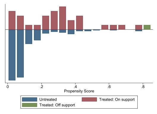
came safer ex post. To account for the longer time it takes for delinquency to occur, an
alternative difference-in-difference setup is used to compare RMBS-only securitizers and banks
that are mortgage sellers in an extended sample period. Both ordinary least squares (OLS) and
propensity score matching yield similar results. The higher ex ante risk of the loans represented
by higher wisk-weighted assets ratio and their better ex post performance are consistent with
banks exerting more effort to screen and monitor borrowers after the implementation of the
retention rules. Overall, there was a simultaneous increase in bank screening/monitoring and
risk shifting, and according to the model, this happens only when the current rate of 5% is
overshooting.
Lastly, I extend the model to discuss the implications of my results for the optimal reten-
tion form. In the final rule of the retention requirements, banks can retain either a horizontal
interest, consisting of the most subordinated tranches, a vertical interest in each class of ABS
tranches, or a combination of both. I show first that the trade-off between monitoring and gam-
bling exists under both retention forms. Second, the horizontal component generates a higher
expected value for the bank when the additional capital requirement brought by subordinated
tranches is not a constraint. Finally, I show that at a fixed retention ratio, horizontal retention
leads to greater borrower monitoring by the bank after securitization, but also increases the
likelihood of over-regulation and risk shifting. This is due to the fact that the larger fraction of
the loan retained under horizontal retention effectively resembles an increased retention ratio.
From a welfare perspective, the choice of optimal retention form presents yet another trade-off.
Ultimately, the findings of this paper have important implications for regulators and practi-
tioners in the banking and financial sectors as they seek to balance these competing objectives
in designing policies for securitization.
Related literature. This paper connects several different strands of literature. The first
literature studies how securitization negatively affects banks’ traditional roles. Theoretically,
Pennacchi (1988), Gorton and Pennacchi (1995), Petersen and Rajan (2002), and Parlour and
Plantin (2008) argue that securitization leads to a decline of the originating bank’s screening
and monitoring incentives. Empirically, Keys et al. (2010) and Purnanandam (2011) show
3that securitization led to lax screening standards of mortgages; Piskorski, Seru, and Vig (2010)
and Agarwal et al. (2011) provide evidence that securitization damaged servicing of loans, in
particular renegotiation of delinquent loans. I contribute to this literature by analyzing the
relationship between securitization and risk shifting.
The second literature discusses the optimal retention form, that is, which tranches banks
should retain in response to retention requirements. Fender and Mitchell (2009) and Kiff and
Kisser (2014) discuss the optimality of equity and mezzanine tranches in maximizing screening
efforts. Pagès (2013) finds that to implement optimal delegated monitoring by the bank, the
securitization scheme should use a cash reserve account rather than retention of the residual
interest. Malekan and Dionne (2014) study the optimal contract with regard to retention in
the presence of moral hazard in lender screening and monitoring. In those papers, the retention
requirement is fixed. Instead, I study the optimal requirement, and my results hold under
different retention forms. The optimal retention form is also discussed under the broader
concept of moral hazard.
This paper is also related to the large literature on risk shifting uncovered by Jensen and
Meckling (1976). For an early literature review, see Gorton and Winton (2003). Keeley (1990),
Demsetz, Saidenberg, and Strahan (1996), and Repullo (2004) demonstrate the negative first-
order effect of profitability on risk shifting. The focus of this literature is mainly capital
requirements. This paper instead sheds light on risk shifting and retention requirements in
securitization.
Moreover, this paper contributes to the relatively small empirical literature on the impact
of retention rules. Furfine (2020) shows that after the implementation of the retention rules,
loans in the commercial mortgage-backed securities (CMBS) market become safer, as measured
by indexes such as interest rates, loan-to-value ratios, and income-to-debt-service ratios. In a
similar manner, Agarwal et al. (2019) find that underwriting standards in the CMBS market
are tighter after the implementation of the final rules. The results in the two papers supplement
my empirical findings on banks’ monitoring and screening behavior, but they do not capture
the risk-shifting aspect.4
Lastly, there is a literature about signaling private information through retention, pioneered
by Leland and Pyle (1977) and DeMarzo and Duffie (1999). Guo and Wu (2014) argue that
mandatory retention may deteriorate the adverse selection problem because it prevents issuers
from using the level of retention as a signal. On the other hand, Flynn, Ghent, and Tchistyi
(2020) show that banks can in fact signal through the retention structure of vertical and hori-
4
In a related paper, Sarkisyan and Casu (2013) show that retained interests increased bank insolvency risk
before the crisis.
4zontal interests. The retention policy is fixed in those papers. This paper examines the optimal
policy but does not contain signaling. In Chemla and Hennessy (2014), screening is combined
with a follow-up possible signaling process through junior tranches, and optimal retention form
is also discussed. But in their paper the retention requirement is fixed and there is no risk
shifting.
Layout. The paper proceeds as follows. Section 2 describes the institutional background
of securitization and risk retention. Section 3 introduces the model, and Section 4 tests its
predictions. Section 5 extends the model, and Section 6 concludes the paper.
2 Institutional Background
In a standard securitization process, a loan originator determines whether a borrower qualifies
for a loan and, if so, the interest rate of the loan. The originator sells it to an issuer (sometimes
referred to as sponsor), who brings together the collateral assets from originators for the asset-
backed security.5 The issuer pools assets together and sells them to an external legal entity,
often referred to as a special-purpose vehicle (SPV). The structure is legally insulated from
management. The SPV then issues security, dividing up the benefits (and risks) among investors
on a pro-rata basis. The issuer usually keeps the servicing rights, that is, the responsibility
for managing payments and working closely with the trustee, who represents investors. Credit
enhancements are also provided by the issuer to protect investors from potential losses on
the securitized assets, the most common forms being subordination, overcollateralization, and
excess spread.
AAA AAA
AA AA
... ...
Equity Equity
Vertical Horizontal
Figure 1: Retention options
5
The banks I study simultaneously serve as issuers and originators of the portfolio of securitized assets.
5In October 2014 after the crisis, to better align the incentives involved in the securitization
process, the SEC, FDIC, Federal Reserve, OCC, FHFA, and HUD adopted a final rule (the Final
Rule) implementing the requirements of Section 15G of the Exchange Act, which was added
pursuant to Section 941 of the Dodd-Frank Act. The Final Rule requires an issuer of ABS
to retain at least 5% of the credit risk related to that securitization and restricts the transfer,
hedging, or pledge of the risk that the sponsor is required to retain. The issuer must retain
either an eligible vertical interest (an interest in each class of ABS interests issued as part of the
securitization), horizontal interest (the issuer holds the most subordinated claim to payments of
both principal and interest transactions), as shown in Figure 1, or a combination of both so long
as the combined retention is not less than 5% of the fair value of the transaction. For the eligible
horizontal interest option, the amount of the required risk retention must be calculated under
a fair value approach under generally accepted accounting principles (GAAP). The Final Rule
came into effect in December 2015 for RMBS and December 2016 for other ABS. A similar
retention rule has been introduced by the EU, covered by Article 2(1) of the Securitization
Regulation.
Some exemptions exist for particular categories of securitization in the Dodd-Frank Act.
For example, ABS or the pooled assets that have the benefit of government guarantees are
exempted; sponsors of securitization pools that are solely composed of qualified residential
mortgages, as defined by the Consumer Financial Protection Bureau (CFPB) under the Truth
in Lending Act, are not required to retain any risk; and collateralized loan obligation (CLO)
managers are not subject to risk retention due to a court ruling in 2018. Beyond that, Section
15G permits the agencies to adopt other exemptions from the risk retention requirements for
certain types of ABS transactions.
3 The Model
This section presents the main model. I illustrate how mandatory retention in the securitization
process affects banks’ decisions and market outcomes. I use uppercase letters to represent banks’
decision variables, while parameters are denoted using lowercase and Greek letters. The model
of this section assumes that banks use a vertical retention form for exposition and simplicity
(see Section 2 for a discussion of retention form), but Section 5 shows that the main results are
unchanged when banks can use both forms of retention.
63.1 Model Setup
Model overview. Consider an economy with a bank and multiple investors, both assumed to
be risk-neutral. The economy lasts for four dates: t ∈ {0, 1, 2, 3}. At t = 0, the bank needs
to invest one unit of money in a project using equity e and debt d = 1 − e. The bank chooses
between two projects: a good project and a bad (gambling) project, the details of which will
be defined later. At time 1, the bank securitizes a fraction of its project to investors. The
securitization process is regulated by mandatory retention requirements, which will also be
specified below. At time 2, the bank chooses whether to monitor its project M ∈ {0, 1}, where
M = 1 denotes monitoring and M = 0 denotes no monitoring. The monitoring effort affects
the credit risk of the project as a whole, not just the portion the bank retains. At time 3,
returns are realized. The timeline of the model is in Figure 2.
0 1 2 3
Bank chooses Bank securitizes Bank chooses Returns realized;
between projects subject to retention whether to monitor cash flows paid out
requirement
Figure 2: Timeline of the events
Risk-shifting problem. At time 0, the bank faces a risk-shifting problem (Jensen and Meck-
ling, 1976) when it chooses which project to invest in: K ∈ {g, b}. The term “project” can
be interpreted as the bank’s portfolio of investments. The expected return of a project de-
pends on monitoring, but for any level of monitoring, the good project g has higher expected
returns. Meanwhile, the bad project b yields higher private returns if the gamble pays off. More
specifically, given a monitoring level M ∈ {0, 1}, the project payoffs are
Rg w/prob qg (M ) Rb w/prob qb (M )
Payoff Payoff
good project = , bad project =
r otherwise r otherwise
where Rb > Rg > 1 > r, and
qg (M ) = pg − (1 − M )∆g ,
qb (M ) = pb − (1 − M )∆b ,
with pg > pb . To clarify, when the bank opts to monitor (M = 1), the success probabilities for
the projects are just pg and pb , and the project payoffs are
Rg w/prob pg Rb w/prob pb
Payoff (M =1) Payoff (M =1)
good project = , bad project = .
r otherwise r otherwise
7When the bank chooses not to monitor (M = 0) at time 2, the probability of success for a
project drops by ∆K , and the project payoffs are
Rg w/prob pg − ∆g Rb w/prob pb − ∆b
Payoff (M =0) Payoff (M =0)
good project = , bad project = .
r otherwise r otherwise
I assume ∆g < ∆b , meaning that without monitoring, the good project’s success probability
decreases less than the bad project’s. This implies the bad project’s success probability is
always lower, qb (M ) < qg (M ) for any M .
I make two further assumptions. First, I assume that if the cash flow r is realized, the bank
fails and r can be considered as the liquidation value of the bank. For simplicity, I assume
r = 0 in this section and relax that assumption in Section 5. And without loss of generality, I
normalize pg = 1.6 The stochastic returns of the two projects are then assumed to satisfy
Rb > Rg > pb Rb > 1.
The first inequality corresponds to the fact that the gambling project yields a higher payoff in
the success state, and the second inequality corresponds to the fact that the good project has a
higher expected return at any monitoring level.7 The last inequality states that both projects
have positive NPV.
If the bank is solvent at time 2, it repays d to debtholders. The bank has limited liability.
When the gamble fails, the cost is borne by debtholders. I make the following assumption that
the amount of debt the bank needs to repay, d, is not too small.
Rg −pb Rb
Assumption 1 d > 1−pb
.
This assumption guarantees that risk shifting is possible, at least when the bank retains every-
thing on the balance sheet, that is, pb (Rb − d) > Rg − d.
Securitization and mandatory retention. At time 1, the bank securitizes an exogenous
fraction α of its project, which is then repackaged into multiple securities or “tranches” with
varying seniorities. The most junior tranche will be the first to absorb losses, followed by
subsequent tranches in order of seniority.8 Throughout this paper, the securitized fraction of
the project will be referred to as the “pool.”
6
This assumption implies that when m = 1, the good project is riskless.
7
To see this, note that Rg > pb Rb implies (1 − ∆g )Rg > (pb − ∆b )Rb .
8
It should be noted that the design of these securities, or subordination in practice, is considered exogenous
and will not be the focus of this paper. See Mitchell (2004) for an overview of tranching and related literature
on security design.
8The securitization process is regulated by mandatory retention requirements: the bank
chooses to retain Z fraction of the tranches such that the retained tranche value is no less than
θ fraction of the market value of the pool. The policymaker sets θ. In the vertical retention we
focus on in this section, the bank simply holds each class of the tranches; hence, the retention
constraint is
Z ≥ θ,
that is, the bank needs to retain at least θ fraction of the pool.
Competitive investors observe the bank’s project choice K and retention choice Z, and bid
a price (schedule) P .9 The total monetary benefit of securitization for the bank at time 1 is λP ,
where λ > 1 is the gain from trade. It can be interpreted, for instance, as lower funding costs
in extending new loans, or new investment opportunities, which I do not model preciesely, or
an increase in reported profit that is related to the compensation of the CEO. Moreover, λ > 1
is equivalent to the bank discounting future cash flows at a higher rate than investors (e.g.,
DeMarzo and Duffie, 1999). One underlying assumption here is that the cash flows generated
from securitization are primarily used either for future business operations or as dividends to
shareholders. This assumption can be relaxed to allow for a partial allocation towards the
repayment of existing debts (d), but not for the complete repayment.10
Monitoring. At time 2, the bank chooses whether to monitor: M ∈ {0, 1}. The influence
of this choice on stochastic returns is presented above. The monitoring process incurs a cost,
denoted as c, applicable to both project types.
Equilibrium definition. I present the definition of equilibrium in this model.
Definition 3.1 (Equilibrium.) The equilibrium consists of the bank’s project choice K at
time 0; the bank’s retention choice Z at time 1; price P of the tranches sold to investors; the
bank’s monitoring choice M at time 2, such that P reflects seniorities and project and retention
choices. Investors break even and the bank maximizes its value sequentially subject to retention
constraint at time 1.
9
The project choice being observable to securitization purchasers is in accordance with ABS-offering prospec-
tuses that provide detailed information on the underlying collateral assets, as governed by Regulation AB from
2005 and reinforced in Dodd-Frank. And the transparency of the retention choice is governed by the retention
rules.
10
If all cash flows were used solely for debt repayment, the bank would monitor more when there is less
retention, due to λ > 1. The intended consequences of mandatory retention rules cannot be achieved. Therefore,
I exclude this possibility from my analysis.
9In the subsequent sections, for the sake of clarity and ease of exposition, the subscript K in
pK , RK and ∆K will be omitted, provided that does not result in any ambiguity.
3.2 Monitoring decision
The model is solved backwards. In this section, I solve for the bank’s monitoring decision
at time 2, after the securitization stage. Given the project and retention choices (K, Z), the
optimal monitoring decision maximizes the bank’s residual profits net of monitoring costs:
Π2 (K, Z) = max qK (M ) (1 − α)R + ZαR − d − cM.
M ∈{0,1}
In the expression, when the investment is successful, (1−α)R is the value of the non-securitized
part of the project, ZαR is the value of the tranches retained on the bank’s books, and d is the
amount of debt the bank repays being solvent. I present the solution.
Proposition 3.1 Given (K, Z), the bank chooses M = 1 if and only if
c
∆
+ d − (1 − α)R
Z ≥ Z̄K ≡ .
αR
Proof: All the proofs are presented in Appendix A.
Here I assume that the bank monitors when there is a tie. The bank monitors if the
loan retained on the balance sheet is large enough, that is, if there is “skin in the game.”11
The threshold Z̄K is increasing in the inverse of the efficiency of the monitoring technology,
c
measured by ∆
, and total debts d it owes: when the monitoring technology is highly efficient,
the bank will advance its monitoring decision to increase profits. Conversely, if the bank owes
significant debts (higher leverage), it may hesitate to monitor because the benefits of being
solvent may be outweighed by the costs of paying off the debts. The threshold is decreasing in
the project return RK . If the bank chooses the bad project (with Rb > Rg and ∆b > ∆g ), it
has more incentive to monitor. Put another way, Z̄g > Z̄b . Monitoring and gambling are hence
complements.
3.3 Securitization problem at time 1
In vertical retention, investors purchase from the bank 1 − Z fraction of the pool and share the
default risk of the underlying project evenly in terms of seniority with the bank. If the bank
11
To further illusatrate the point in footnote 10, when cash flows generated from securitization (which will
be λαZR as shown later) are used entirely for debt repayment, one can show that contrary to the result above,
the bank monitors if and only if Z is below some threshold.
10goes bankrupt, the debtholders will take over the tranches. Although the transaction takes
place before the monitoring stage and the bank cannot commit to monitoring, investors who
observe Z can later infer the bank monitoring decision by comparing it to Z̄K and pay the
corresponding adjusted price. Specifically, for a given project, the schedule of prices investors
offer based on Z and rational expectations is
(
(1 − Z)αpR if Z ≥ Z̄K ,
P (Z|K) =
(1 − Z)α(p − ∆)R if Z < Z̄K .
The expected value of the pool will be αpR if there is subsequent monitoring and α(p − ∆)R
if there is not.
The bank’s Bellman equation at time 1 is expressed as follows:
Π1 (θ|K) = max λP (Z|K) + Π2 (Z|K)
Z
s.t. Z ≥ θ.
Here, the total monetary benefits of securitization are represented by the product of λ and
P (Z|K). The retention requirement is captured by the inequality constraint. In the vertical
retention, the bank only needs to retain a fraction larger than θ of the pool. I first characterize
the shape of the bank’s objective function as a function of Z.
Proposition 3.2 The bank’s objective function λP (Z|K) + Π2 (Z|K) is upper semicontinuous
at Z̄. Moreover, it is linear and decreasing in Z on [0, Z̄K ) and [Z̄K , 1].
To make monitoring indeed a friction, I assume for each project K the following holds.
Assumption 2 λ ∆R − pd < c for both projects.
To have enough incentive to monitor, the bank must retain at least Z̄K of the project. While
monitoring improves project quality, it comes at a cost: lowered securitization revenue due to
retention and the cost of monitoring. This assumption guarantees that in equilibrium, the bank
chooses zero retention in the absence of mandatory retention rules. However, if this assumption
is violated, the bank always chooses to retain Z = Z̄K and monitor. In this case, there is no
need for regulation to address the misaligned incentive of monitoring. The left side of Figure
3 illustrates the bank’s objective function under this assumption, with the second piece of the
function being steeper than the first.
11bind-
ing slack binding
0 Z̄K Z 0 ZK Z̄K Z
Figure 3: The bank’s objective function and retention constraint
We are now ready to impose the retention constraint. Let ZK be such that
λP (ZK |K) + Π2 (Z̄K |K) = λP (Z̄K |K) + Π2 (Z̄K |K).
According to the shape of the objective function, this ZK exists and is smaller than Z̄K , as
shown in the right part of Figure 3. In fact, the formula of ZK for project K is
(λp − (p − ∆))(R − d) − (λ − 1) ∆c − c
ZK = 1 − . (1)
(λ − 1)α(p − ∆)R
If the required threshold θ is below ZK , the bank chooses the lowest possible retention, im-
plying that the retention constraint is binding. When the threshold θ is between ZK and Z̄K ,
the objective function is maximized at Z̄K , indicating that the retention constraint is not bind-
ing. However, if θ is above Z̄K , the constraint is binding again since the objective function is
decreasing. These are summarized by the following result.
Proposition 3.3 (Retention choice.) The bank’s optimal retention choice of Z is
θ if θ < ZK ,
Z(θ|K) = Z̄K if ZK ≤ θ < Z̄K ,
if Z̄K ≤ θ.
θ
If there is no retention requirement, the bank will not make any monitoring efforts. The
policymaker can set the lower bound θ of the retention requirement to ZK to encourage moni-
toring from the bank, which we show later to be part of the socially optimal allocation. Since
ZK is smaller than Z̄K , the policymaker only needs a small lower bound of θ.
Proposition 3.4 (More retention leads to more monitoring.) Given a project K, the
policymaker can set θ ≥ ZK to implement monitoring. In particular, if the policymaker sets
(λ − (1 − ∆g ))(Rg − d) − (λ − 1) ∆cg − c
θ ≥ Zg ≡ 1 − ,
(λ − 1)α(1 − ∆g )Rg
the bank always monitors.
12For a given project K, under the optimal retention choice, the bank’s expected value Π1 (θ|K)
is graphed in Figure 4. It is constant on [ZK , Z̄K ] because of the slack retention constraint.
The second part of the result comes from the fact that the good project has a larger ZK .
Π1 (θ|K)
bind- binding
ing slack
0 ZK Z̄K θ
Figure 4: The bank’s expected value under the optimal retention choice
3.4 Risk shifting at time 0 and equilibrium
In this section, I complete the equilibrium characterization by studying the bank’s risk-shifting
motives in the presence of limited liability, which imposes more costs on creditors in bad out-
comes. I show that mandatory retention increases the bank’s risk-shifting propensity, defined
by the difference between the values of gambling and being good concerning project choice.
At time 0, for a required retention ratio θ, let the bank’s expected value of choosing the good
project be Vg (θ) ≡ λP (Zg (θ)|g) + Π2 (Zg (θ)|g). The retention Zg (θ) comes from Proposition
3.3. Similarly, if the bank shifts risk, its value changes to Vb (θ) ≡ λP (Zb (θ)|b) + Π2 (Zb (θ)|b).
The bank hence solves
max VK (θ).
K
To solve this, I define the gain from risk shifting as
G(θ) ≡ Vb (θ) − Vg (θ),
and the bank chooses to gamble if G(θ) > 0. The equilibrium depends on the behavior of
this gain function under the different requirements of θ. Note that this function has four kink
points since both Vg (θ) and Vb (θ) have two: Zg , Z̄g and Zb , Z̄b , as shown in Figure 4. I make
the following assumption so that in equilibrium it is possible for the bank to optimally choose
the good project and monitor it at the same time.
Assumption 3 (λ − 1)c ∆1g − ∆pbb > λ[pb (Rb − d) − (Rg − d)].
13It guarantees that Vg (Z̄g ) > Vb (Z̄b ): that is, when both retention constraints are slack, if the
bank starts to monitor the good project, it obtains a higher value from that project than from
gambling. The main result of the paper is the following.
Proposition 3.5 (Equilibrium) There exist two thresholds θ, θ̄ with θ < θ̄ such that the bank
chooses the good project but does not monitor for θ < θ; the bank chooses the good project and
makes an effort to monitor for θ ∈ [θ, θ̄]; the bank gambles and monitors subsequently for θ > θ̄.
The above equilibrium characterization implies that at a high retention ratio θ, the bank
starts to gamble. Because the gambling project has lower NPV than the good project, the total
output is lower. This is the unintended consequence of mandatory retention rules.
Corollary 3.1 (Unintended consequence of mandatory retention.) The bank starts to
gamble when θ > θ̄.
The two possibilities of Vg (θ), Vb (θ), and the corresponding G(θ) are portrayed in Figure
5. At a low retention ratio, the bank chooses the good project because it has favorable market
value and hence is easy to securitize; and this is the driving force of G(θ) being monotonic
increasing on some region. As the retention ratio increases, the value of choosing the good
project is hurt more because of the higher gain from trade generated. When the retention ratio
is high enough, limited liability and higher upside return Rb make the gambling project more
profitable.
Vb (θ) Vb (θ)
Vg (θ) Vg (θ)
G(θ) G(θ)
0 θ
0
θ̄ θ θ θ̄ θ
not monitor monitor not monitor monitor
Figure 5: Risk-shifting propensity
It is worthwhile to compare the outcomes of the two other scenarios: selecting the good
project without monitoring, and selecting the gambling project with monitoring. I assume that
pb > 1 − ∆g .
14That is, the default rate is lower when there is monitoring despite some risk being shifted.
First, this is consistent with the narrative that lax monitoring in securitization leads to bad
loans and the global financial crisis. Moreover, it also matches the empirical evidence explored
later showing that the mandatory retention rule has caused banks to monitor and gamble
simultaneously, but loan delinquencies have dropped.
3.5 Welfare and optimal retention requirement
This section provides the welfare analysis and discusses the optimal retention ratio. The total
welfare is defined as the sum of the payoffs of all players12 as a function of θ. Since investors get
zero in expectation, the sum is just the bank’s value V bank plus debtholders’ expected return
p(θ)d, where p(θ) is the probability of the equilibrium project being successful. In other words,
W (θ) = V bank (θ) + p(θ)d,
where
(
Vg (θ) if θ ≤ θ̄,
V bank (θ) =
Vb (θ) if θ > θ̄,
according to Proposition 3.5 and
1 − ∆g if θ ≤ Zg ,
p(θ) = 1 if θ ∈ [Zg , θ̄],
pb if θ > θ̄.
Note that V bank (θ) is continuous but p(θ) is not. After rearrangements, the welfare can be
written as
W (θ) = 1 + (λ − 1)α(1 − Z(θ)) R̄(θ)–c(θ),
which is the sum of total output and the net gain from securitization less the potential moni-
toring cost. The shape is shown in Figure 6.
There are jumps at Zg and θ̄ because p(θ) has jumps at these points. Since securitization
brings gains of trade, a higher retention ratio reduces securitization levels and, hence, brings
down the total welfare. This is why the welfare is decreasing on each piece, except for [Zg , Z̄g ],
on which the retention constraint is slack. In fact, if we impose the following assumption, the
welfare is maximized at [Zg , Z̄g ] and maximized when the good project is chosen and monitoring
effort is delivered:
12
That is, equal Pareto weights are attached to each player.
15over-regulating
0 θ ZgM θ̄ θ
Figure 6: Welfare
Assumption 4 (λ − 1)[1 − α(1 − ∆g )] + ∆g Rg − (λ − 1)d > c + (λ − 1) ∆cg .
This assumption is only about the good project; hence, it is easy to satisfy when, say, Rg is large
enough. Similar to the benchmark case, the social monitoring cost and loss of gains from trade
due to retention are low compared to the additional social benefits generated from monitoring
the good project. As λ converges to 1, the above assumption converges to ∆g Rg > c. Since
θ = Zg , we have the following result.
Proposition 3.6 (Optimal retention.) The optimal retention ratio is [θ, Z̄g ]. On this range
of θ, the bank invests in the good project and monitors, and the retention constraint is slack.
The optimal retention ratio is interior, meaning that a certain degree of retention is the
correct policy. Mandatory retention has three effects: it induces monitoring, it encourages risk
shifting if the degree of retention is very high, and it restricts securitization activities and hence
reduces the gains from trade. What happens when θ is between Z̄g and θ̄? In this region,
the bank still chooses the good project and delivers monitoring effort according to Proposition
3.5; however, its securitization activities are over-regulated. In summary, welfare is maximized
when the good project is selected and just monitored, without securitization activities being
overly regulated.
Two remarks are worth making. First, if the policymaker places a 100% Pareto weight
on debtholders, total welfare is simply p(θ), the probability of success. The optimal retention
ratio is [θ, θ̄]. Second, the policymaker is imposing an inequality constraint. If this inequality
constraint is replaced with an equality constraint, that is, the bank has to retain θ fraction
of the pool, the optimal retention is unique: θ∗ = Z̄g . This is the lowest level of retention to
incentivize the bank to monitor. And the policymaker does not want to go beyond that to over-
regulate securitization. Since Z̄g is larger than θ, Z̄g can be close to θ̄, above which the bank
16shifts risk. Therefore, choosing an inequality retention constraint provides the policymaker
with more flexibility to balance monitoring and risk shifting.
3.6 Model predictions
This section connects the above results with empirical tests in the next part of the paper. The
model provides sharp predictions about the link between policy and unintended consequences,
which is summarized in Table 1. In particular, if we observe no changes in monitoring and risk
shifting, it implies that the current retention ratio is below the optimal level. Similarly, if we
observe a simultaneous increase in monitoring and risk shifting, the current retention ratio is
13
too high.
Monitor Shift risk
θ θ̄ Y Y
Table 1: Model predictions
As we will demonstrate in the next section, banks do monitor more and shift more risk after
the retention rule’s implementation, implying that the current rate of 5% is overshooting.14
4 Empirical Evidence
This section tests the model predictions. Since risk and capital management are typically
carried out at the highest level, I use US bank holding company (BHC) data from Y-9C forms.
A BHC is defined as a securitizer if it reports at least one non-zero outstanding securitization
activity in the sample period and has at least two years of existence. From 2001Q2, BHCs were
required to detail their securitization activity in their regulatory reports (Schedule HC-S of the
Y-9C report). Securitization activity is the outstanding principal balance of assets sold and
13
Admittedly, since the optimal retention ratio (when the planner places equal weights) [θ, ZgM ] is embedded
in [θ, θ̄], we cannot distinguish between an optimal retention requirement and an over-regulating retention
requirement when monitoring is observed and risk shifting is not in this case.
14
Note that if Assumption 4 fails, the socially optimal retention ratio is 0. This does not change this impli-
cation.
17securitized with servicing retained or with recourse or other seller-provided credit enhancements
in millions of US dollars. If another bank acquired a bank, I remove the non-survivor from the
sample.
I use two measures to document bank risk. The first is the risk-weighted assets (RWA)
ratio, which is calculated by dividing the RWA by the total assets of a bank. To determine a
bank’s RWA, its assets are categorized by risk level and the likelihood of causing a financial
loss. In simplified terms, the RWA ratio is computed as follows:
Pn
k=1 ωk Ak
RWA ratio = P n ,
k=1 Ak
where ωk denotes the risk weight of asset k and Ak denotes the value of asset k. If the ωk values
are fixed, investing in assets with higher risk weights will increase the numerator while keeping
the denominator constant. Therefore, an increase in the RWA ratio indicates that the bank is
allocating more resources to riskier projects, or engaging in risk shifting.15
The second measure is the securitization delinquency ratio, defined as
loans 90 or more days past due + (loans charged off)
DEL = .
lagged total loans outstanding
The delinquency rate measures the fraction of loans outstanding that are non-performing loans;
hence, it is an ex post index of bank risk.
I use two difference-in-difference (DID) setups to show a notable rise in the RWA ratio for
RMBS securitizers and a decline in the loan delinquency rate following the implementation of
the retention rules. The first DID estimation compares US BHC RMBS securitizers to other
BHC securitizers from 2015Q1 to 2016Q4, where the mandatory retention rule took effect for
RMBS in December 2015, and one year later for all other categories of securitization.16 However,
since delinquency takes place at least 90 days after a loan is generated, a short sample period
may not yield accurate estimates. Therefore, I also consider an alternative DID design with a
longer horizon (2014–2017) and compare RMBS-only BHC securitizers to non-securitizers who
are mortgage sellers.
15
In the US Basel framework Final Rule, there are two implementation approaches to calculate RWA. The
standard approach, which applies to all banks, attaches fixed risk weights to multiple exposure types. In the
advanced approach, which applies to banks with consolidated assets greater than $250 billion, exposures are
broadly classified into four categories: retail, wholesale, securitization, and equity. In addition, the internal
ratings-based (IRB) formula applies to retail and wholesale exposures. The standard and advanced approaches
took effect in January 2015 and January 2014, respectively. Banks with total assets greater than $250 billion
have to calculate RWA using both standardized and advanced approaches and may act differently from the rest
of the banks.
16
While the Dodd-Frank Act was passed in July 2010, the final rule of mandatory retention was, in fact, not
agreed upon until October 2014. There was then a two-year delay between the agreement and implementation.
184.1 DID: RMBS securitizers versus other securitizers
In the first DID setup, the focus is the effect of the retention rules on banks’ risk-shifting
behavior, measured by an increase in the RWA ratio. I use US BHC data from 2015Q1 to
2016Q4 from Y-9C forms.
As mentioned in footnote 15, banks with consolidated assets greater than $250 billion report
RWA using two different approaches. I first remove those banks and add them back as a
robustness check. There are 52 BHC securitizers and 359 bank-quarter observations. Banks
that issue RMBS may also be involved in other categories of securitization businesses. I consider
the standard binary treatment as well as a continuous treatment.
In the binary treatment, banks are split into control and treatment groups. The control
group contains 12 BHC securitizers that do not issue RMBS. The treatment groups are banks
that issue RMBS, but with different issuance shares, defined as
RMBS activities
Share = .
Total securitization activities
The RMBS activities, as well as total securitization activities, do not contain loans sold to other
institutions or entities.17 I consider three definitions of the treatment group: (1) share > 0.5
every quarter; (2) share > 0.8 every quarter; (3) share = 1 every quarter. There are 40 banks
in total that are RMBS issuers: 37 of them are in group 1, 36 in group 2, and 33 in group 3.
Securitization activities and shares are stable across time for RMBS securitizers. There is one
single bank that did not issue RMBS until 2016Q3, and its share is below 0.15.I hence include
this bank in the control group. After defining the variable Dit to equal 1 if bank i is an RMBS
securitizer after December 2015 and 0 otherwise, the benchmark model can be expressed as the
following fixed-effect panel regression:
RW Ait = ZDit + Xit′ δ + αi + γt + ϵit , (2)
where subscripts it uniquely identify individual observations for bank i in quarter t. The
dependent variable is the RWA ratio. I include bank fixed effects to absorb unobservable
differences in bank business models and time fixed effects to absorb macro-economic shocks
such as quantitative easing. The independent variable γt is time fixed effects, Xit is the set
of bank-specific control variables, αi is the individual fixed effects, and ϵit is the error term.
17
Examples of other institutions and entities are the Federal National Mortgage Association (Fannie Mae) or
the Federal Home Loan Mortgage Corporation (Freddie Mac). These government-sponsored agencies, in turn,
securitize these loans and are not subject to the mandatory retention. These items are reported separately in
Items 11 and 12 in Schedule HC-S.
19Standard errors are clustered at the bank level. The coefficient of interest is Z. I estimate (2)
with and without bank-specific controls.
To shed light on the dynamics of the average treatment effect before and after the passage
of the mandatory retention rule, I replace the dummy Dit in specification (2) with leads and
lags, which I name as Bef ore and Af ter. The new regression model is
4
X 3
X
RW Ait = αi + Z5−N BN,it + α3−M AM,it + Xit′ δ + Ct + ϵit , (3)
N =2 M =0
where BN denotes N periods before the treatment and AM denotes M periods after treatment.
The quarter before treatment is used as the benchmark. The coefficients Z to α estimate
the average changes in banks’ risk in the quarters preceding and following the Final Rule’s
implementation. The aim here is to test whether the effect is isolated to periods occurring only
after the onset of the implementation.
The set of bank-specific control variables includes on-balance-sheet and off-balance-sheet
items. On-balance-sheet items include some standard explanatory variables in the banking
literature, like size (measured by the log of total assets), profitability (measured by return on
assets), capital buffer (measured by the difference between banks’ regulatory risk-based capital
and the minimum required capital ratio), and liquidity ratio (over total assets). Banks of
different sizes are regulated with different stringencies. For example, banks with assets of more
than $50 billion are subject to stress tests, must submit resolution plans, and have tighter
liquidity requirements. The capital buffer and liquidity buffer are a sign of bank solvency and
stability. The off-balance-sheet item I use is securitization activities scaled by total assets.
20Table 2: Summary statistics
Control group RMBS share≥0.8 RMBS share=1
Variables Mean Std Dev Mean Std Dev Mean Std Dev
Total assets ($ billions) 66.897 63.088 39.754 58.132 26.591 37.946
RWA ratio 0.780 0.119 0.749 0.092 0.748 0.089
RWA ratio (exclude securitization exposure) 0.776 0.119 0.748 0.091 0.748 0.089
Loan ratio (of total assets) 0.646 0.165 0.691 0.100 0.698 0.089
Home mortgage (of total loans) 0.226 0.151 0.322 0.171 0.325 0.180
Consumer loans (of total loans) 0.168 0.162 0.081 0.099 0.080 0.104
C&I loans (of total loans) 0.232 0.124 0.180 0.102 0.177 0.105
Capital buffer 0.101 0.134 0.138 0.915 0.149 0.982
Deposit ratio 0.419 0.186 0.587 0.112 0.597 0.101
Liquidity ratio 0.207 0.104 0.216 0.075 0.213 0.077
ROA 0.009 0.013 0.006 0.005 0.006 0.005
Securitization-assets ratio 0.142 0.340 0.129 0.161 0.122 0.161
Number of banks 12 40 33
Notes: The table presents descriptive statistics of the control group and treatment groups from 2015Q1 to 2016Q4. I report
treatment groups with an RMBS activity share greater than 0.8 as well as equal to 1. The table contains means and standard
deviations of bank characteristics. The RWA ratio is the risk-weighted assets to total assets ratio. ROA is the ratio of net income
to total assets. The securitization-assets ratio is the ratio of securitization activities to total assets. Credit enhancements is the
ratio of total credit enhancements provided by the securitizer to total assets.
The summary statistics for the treatment and control group are reported in Table 2. I
report treatment groups with an RMBS activity share greater than 0.8 as well as equal to 1.
The average total assets of banks in the control group is $60.8 billion, which is greater than
banks in the treatment group, whose average total assets is under $40 billion. Moreover, as
I increase the share of RMBS activities, the average size drops. The average size becomes
$26.6 billion when banks only issue RMBS. Banks in both groups participate in securitization
activities each quarter at levels about 13% to 14% of their size. Regarding on-balance-sheet
items, banks in the treatment group have a slightly higher loan ratio (69% versus 65%) and a
higher home mortgage ratio over total loans (32% versus 23%), which is no surprise. Banks in
the control group focus more on consumer loans and C&I loans. Banks in both groups hold
21% of their total assets in the form of liquid assets. The average RWA ratio in the full sample
is 0.76. Banks in the control group have a higher RWA ratio. The difference between the two
groups is around 0.03 (0.78 versus 0.75). I also report the RWA ratio excluding securitization
exposure. The numbers do not change much. Though operating at a higher asset level, banks
in the control group have more profitable projects than banks in the treatment group (0.009
versus 0.006). As a sign of bank solvency and stability, the average capital buffer in the sample
is 0.11. The treatment group banks are more capitalized than control group banks (0.14 versus
0.10).
21Table 3: The effect of mandatory retention rule on banks’ risk shifting
Dependent variable: RWA ratio
(1) (2) (3) (4) (5)
RMBS≥0.5 RMBS≥0.8 RMBS≥0.8 RMBS=1 RMBS=1
>= $250 billion included
Treatment 0.023* 0.023* 0.021* 0.024* 0.020*
(0.013) (0.013) (0.011) (0.012) (0.011)
Capital buffer 0.001* 0.001* -0.000
(0.000) (0.000) (0.000)
Size -0.097* -0.085 0.020
(0.049) (0.053) (0.040)
ROA 0.720** 0.625* 0.728**
(0.332) (0.342) (0.294)
Liquidity ratio -0.580*** -0.607*** -0.688***
(0.136) (0.119) (0.118)
Securitization-assets ratio 0.077*** 0.069** 0.071***
(0.026) (0.028) (0.024)
Observations 333 325 325 293 325
R-squared 0.083 0.084 0.221 0.208 0.478
Number of banks 49 48 48 45 50
Notes: This table reports the effects of mandatory retention rules on banks’ risk-weighted assets (RWA) ratio, specified by
′
RW Ait = ZDit + Xit δ + αi + γt + ϵit .
Treatment equals 1 if bank i is an RMBS securitizer after December 2015 and 0 otherwise. In the first 4 columns, I increase the
threshold of RMBS activity share from 0.5 to 1. In the first two columns, only bank and time fixed effects are considered. In
columns 3 and 4, bank-specific control variables are added. Banks with total assets of more than $250 billion are removed in the
first 4 columns and added in column 5. Standard errors are in parentheses. The superscripts ***, **, and * represent 1%, 5%, and
10% significance levels, respectively.
Table 3 reports the estimation of equation (2). The first two columns report the results when
no other control variables are included. The treatment groups are defined as RMBS activity
share ≥ 0.5 and 0.8. The RWA ratio of the treatment banks increases 2.3 percentage points
on average and is significantly positive at the 10% level. I increase the activity share threshold
to 1 in column 4, and there is almost no discrepancy between the treatment effect estimates.
As a robustness check, I add back banks with total assets greater than $250 billion and obtain
a similar result, reported in column 5. I report in Table 8 in Appendix C that coefficients are
similar when the dependent variable is replaced with the RWA ratio excluding securitization
exposure. Hence, bank portfolio risk increased outside retained tranches in securitization.
22You can also read