Localization for Lunar Micro-Rovers
←
→
Page content transcription
If your browser does not render page correctly, please read the page content below
Localization for Lunar
                Micro-Rovers
                           Haidar Jamal
                         CMU-RI-TR-21-10
                             May 2021

                    School of Computer Science
                    Carnegie Mellon University
                       Pittsburgh, PA 15213

                       Thesis Committee:
                   David Wettergreen (Chair)
                 William (Red) Whittaker (Chair)
                          Michael Kaess
                           Jordan Ford

Submitted in partial fulfillment of the requirements for the degree of
                  Masters of Science in Robotics

                  Copyright © 2021 Haidar Jamal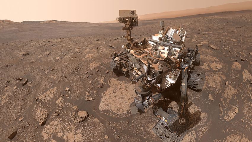
Abstract

This work presents a localization system that enables a lunar micro-rover to navigate au-
tonomously in and out of darkness. This is important for the latest class of small, low-
powered, and fast robots going to the moon in search of polar ice. The first component
of the system is an Extended Kalman Filter that fuses wheel encoding and inertial mea-
surement data. This component does not depend on light or feature-rich terrain and so
can be used throughout the rover’s exploration. The second component is the use of a
sun sensor to provide an absolute heading estimate. The third component is a lightweight
visual odometry algorithm which can be used in lit regions. This component is robust
against slippage, an important concern for any ground vehicle operating on rocky surfaces.
In this thesis, these techniques are described in detail along with their integrated mode of
operation. Testing of the system is demonstrated on physical hardware and its accuracy is
quantified.
Acknowledgements

I would like to thank my first co-advisor David Wettergreen for our meetings where I was
able to explore a variety of hands-on and theoretical topics pertaining to autonomy. His
insight helped me develop as a roboticist, giving me the confidence to develop practical soft-
ware for the MoonRanger team. Furthermore, I would like to thank my second co-advisor
William (Red) Whittaker for trusting me in my role as MoonRanger’s avionics lead. His
leadership and motivation has been hugely inspirational. I grew tremendously in terms
of responsibility and communication from my role. Under Red, I learned how to build a
machine, build it again better, and then again.

I want to thank my team, the soldiers, with whom I suffered and grew with. Thank you
Vaibhav, Daniel, KJ, Jim, Heather, Srini, Jordan, and many others in the MoonRanger
army for the good and the bad times.

I would also like to thank NASA for funding the technology, rover development, and flight
of our mission under LSITP contract 80MSFC20C0008 MoonRanger.

Finally, thank you to my family for your constant support and encouragement.
Here’s the name of the game...

                                 − Red, Day 1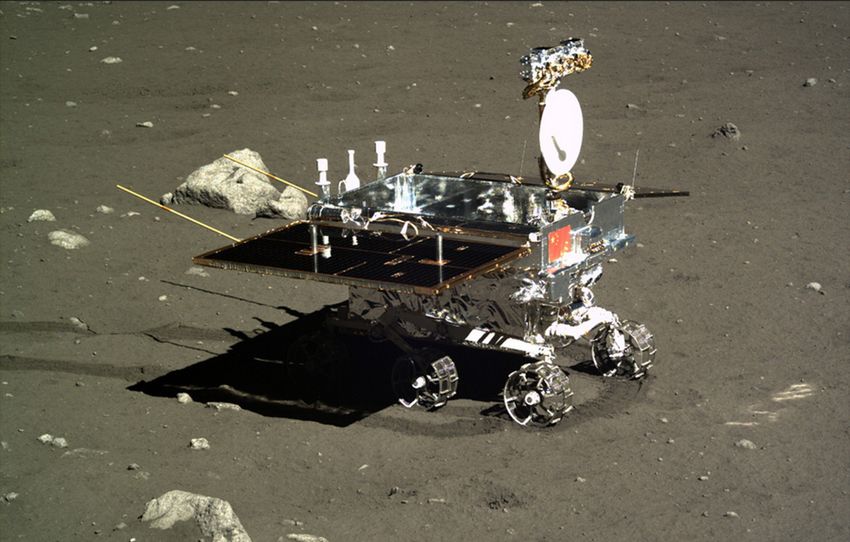
Contents

1 Introduction                                                                                                                                           4

2 Prior Space Rovers                                                                                                                                     6
  2.1 Introduction . . . . . . .    .   .   .   .   .   .   .   .   .   .   .   .   .   .   .   .   .   .   .   .   .   .   .   .   .   .   .   .   .    6
  2.2 Lunokhod 1 . . . . . . .      .   .   .   .   .   .   .   .   .   .   .   .   .   .   .   .   .   .   .   .   .   .   .   .   .   .   .   .   .    6
  2.3 Sojourner . . . . . . . .     .   .   .   .   .   .   .   .   .   .   .   .   .   .   .   .   .   .   .   .   .   .   .   .   .   .   .   .   .    6
  2.4 Spirit and Opportunity        .   .   .   .   .   .   .   .   .   .   .   .   .   .   .   .   .   .   .   .   .   .   .   .   .   .   .   .   .    7
  2.5 Curiosity . . . . . . . .     .   .   .   .   .   .   .   .   .   .   .   .   .   .   .   .   .   .   .   .   .   .   .   .   .   .   .   .   .    9
  2.6 Yutu-1 Rover . . . . . .      .   .   .   .   .   .   .   .   .   .   .   .   .   .   .   .   .   .   .   .   .   .   .   .   .   .   .   .   .   10
  2.7 Pragyan . . . . . . . . .     .   .   .   .   .   .   .   .   .   .   .   .   .   .   .   .   .   .   .   .   .   .   .   .   .   .   .   .   .   10
  2.8 Perseverance . . . . . .      .   .   .   .   .   .   .   .   .   .   .   .   .   .   .   .   .   .   .   .   .   .   .   .   .   .   .   .   .   11
  2.9 Conclusion . . . . . . .      .   .   .   .   .   .   .   .   .   .   .   .   .   .   .   .   .   .   .   .   .   .   .   .   .   .   .   .   .   11

3 MoonRanger                                                                                                                                            13
  3.1 Introduction . . . . . . . . . . . . . . . . . . . . . . . . . . . . . . . . . . . .                                                              13
  3.2 Avionics . . . . . . . . . . . . . . . . . . . . . . . . . . . . . . . . . . . . . .                                                              14
  3.3 Operation . . . . . . . . . . . . . . . . . . . . . . . . . . . . . . . . . . . . .                                                               14

4 A Baseline Position Estimator                                                                                                                         16
  4.1 Introduction . . . . . . . . . . . . . . .                    .   .   .   .   .   .   .   .   .   .   .   .   .   .   .   .   .   .   .   .   .   16
  4.2 Notation . . . . . . . . . . . . . . . . .                    .   .   .   .   .   .   .   .   .   .   .   .   .   .   .   .   .   .   .   .   .   16
  4.3 Extended Kalman Filter . . . . . . . .                        .   .   .   .   .   .   .   .   .   .   .   .   .   .   .   .   .   .   .   .   .   16
  4.4 IMU Sensor Model . . . . . . . . . . .                        .   .   .   .   .   .   .   .   .   .   .   .   .   .   .   .   .   .   .   .   .   17
  4.5 IMU Kinematic Model . . . . . . . . .                         .   .   .   .   .   .   .   .   .   .   .   .   .   .   .   .   .   .   .   .   .   18
  4.6 EKF Prediction Update . . . . . . . .                         .   .   .   .   .   .   .   .   .   .   .   .   .   .   .   .   .   .   .   .   .   18
  4.7 EKF Measurement Update . . . . . .                            .   .   .   .   .   .   .   .   .   .   .   .   .   .   .   .   .   .   .   .   .   20
  4.8 Wheel Encoding to Estimate Position                           .   .   .   .   .   .   .   .   .   .   .   .   .   .   .   .   .   .   .   .   .   21
  4.9 Initialization . . . . . . . . . . . . . .                    .   .   .   .   .   .   .   .   .   .   .   .   .   .   .   .   .   .   .   .   .   21
  4.10 Gravity on the Moon . . . . . . . . . .                      .   .   .   .   .   .   .   .   .   .   .   .   .   .   .   .   .   .   .   .   .   22

5 Sun Sensing                                                                                                                                           23
  5.1 Introduction . . . . . . . . . . . . . . . . . . . . . . . . . . . . . . . . . . . .                                                              23
  5.2 Procedure . . . . . . . . . . . . . . . . . . . . . . . . . . . . . . . . . . . . .                                                               24

                                                            2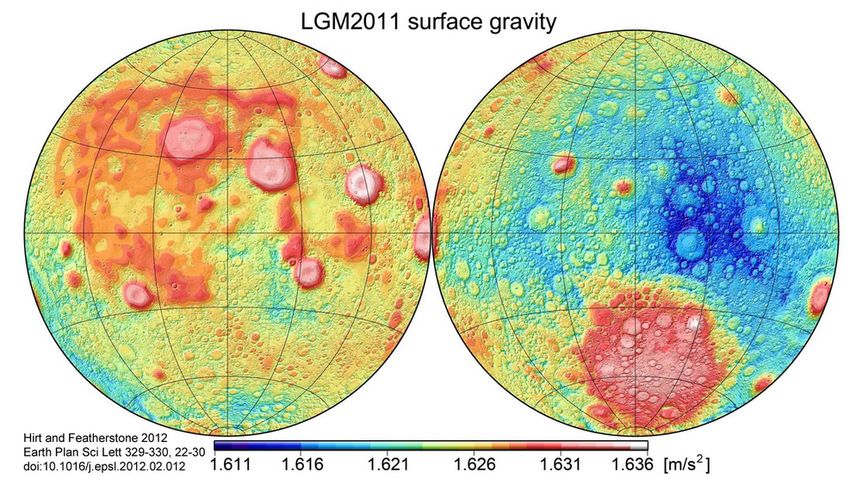
6 Visual Odometry                                                                                                                            26
  6.1 Introduction . . . . . . . . . . . .   .   .   .   .   .   .   .   .   .   .   .   .   .   .   .   .   .   .   .   .   .   .   .   .   26
  6.2 Feature Detection and Matching         .   .   .   .   .   .   .   .   .   .   .   .   .   .   .   .   .   .   .   .   .   .   .   .   26
  6.3 Motion Estimation . . . . . . . .      .   .   .   .   .   .   .   .   .   .   .   .   .   .   .   .   .   .   .   .   .   .   .   .   28
  6.4 GPU Utilization . . . . . . . . .      .   .   .   .   .   .   .   .   .   .   .   .   .   .   .   .   .   .   .   .   .   .   .   .   28

7 System Design and Testing                                                                                                                  29
  7.1 System Design . . . . . . . . . . . . . . . . . . . . . . . . . . . . . . . . . .                                                      29
  7.2 Testing . . . . . . . . . . . . . . . . . . . . . . . . . . . . . . . . . . . . . .                                                    29

8 Conclusion                                                                                                                                 37

                                                 3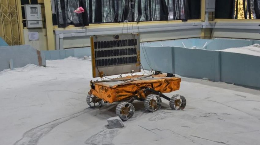
Chapter 1

Introduction

Lunar ice, likely to be found in the greatest abundance near the poles, could be a source
of water for drinking, oxygen for breathing, and for producing propellants for venturing
beyond the moon to deep space. Viability depends on specifics of the accessibility, depth,
and concentration of the ice, which can only be determined by surface missions of repeated
robotic explorations over time. Remote sensing indicates that ice concentrates in low, shad-
owed depressions that may or may not be close to safe landing sites [1]. Navigating through
polar shadows and darkness necessitates capability for pose estimation in the dark without
camera data.

This thesis profiles the pose estimation system designed for MoonRanger, a micro-rover
manifested on a 2022 NASA CLPS flight [2], which will be the first polar mission to per-
form in situ measurement of lunar ice. In its mission, MoonRanger will repeatedly venture
from its initial landing location towards ice targets up to 1 kilometer away as shown in
Figure 1.1. The rover will transmit scientific data points wirelessly to its lander which in
turn will transmit the data to Earth. The scientific data combined with pose estimation
data will provide an accurate map of ice around the landing site that can be used in future
missions. The wireless communication range to the lander will be about 80 meters, pre-
cluding teleoperation and necessitating autonomy for longer drives.

                                             4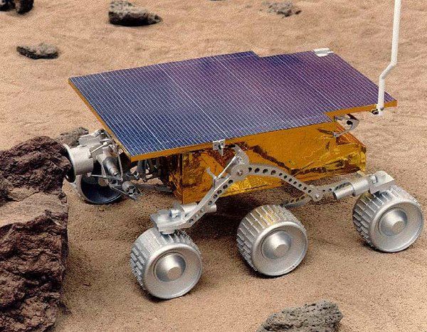
Figure 1.1: MoonRanger will venture towards increasingly further ice targets

With the low incident sun angle at the lunar poles, MoonRanger will repeatedly enter re-
gions of complete darkness throughout its treks. Being a small, solar powered rover, it will
not possess powerful light sources to illuminate its path. Furthermore, the lunar regolith
will likely lead to significant slippage. These various challenges create the requirement of a
robust pose estimation system that can operate in the dark as well as in lit regions, maxi-
mizing the likelihood MoonRanger is able to return to the lander communication range and
transmit its collected data.

The main contributions of this thesis are:

  1. A profiling of the sensing and pose estimation systems of prior space rovers

  2. A discussion on MoonRanger’s avionics with a focus on its sensors

  3. A procedure fusing an inertial measurement unit and wheel encoders

  4. A procedure on using sun sensors to improve heading estimates

  5. A visual odometry pipeline robust against slip

  6. An integrated system for navigation in the lunar poles

  7. Demonstration on physical hardware and evaluation of accuracy on lunar-like terrain

                                              5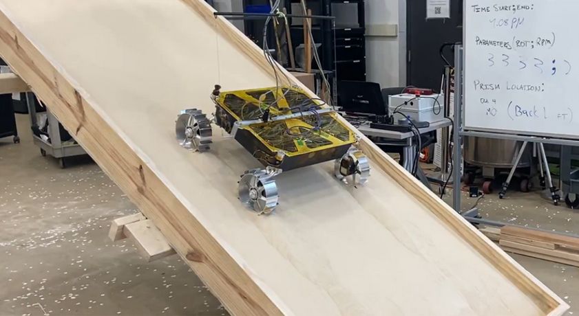
Chapter 2

Prior Space Rovers

2.1    Introduction
In this chapter we describe the computing, sensing, and position estimation algorithms
of prior space rovers. These systems provide a motivation for the development of Moon-
Ranger’s avionics system and localization techniques.

2.2    Lunokhod 1
The Soviet Union’s Lunokhod program launched two rovers, Lunokhod-1 and Lunokhod-2
(Figure 2.1), to the moon in 1970 and 1973, respectively. These were the first rovers to
land on the surface of another celestial body. Each rover carried a directional antenna used
to communicate directly to a ground station on Earth. The rover was teleoperated by a
team of trained drivers and scientists. While driving, the rovers transmitted images, roll
and pitch data, wheel temperature and RPM, currents to wheel motors, and wheel-ground
interaction dynamics [3]. While still, the rover transmitted data of scientific interest. Ac-
cording to [3], ”the navigational system is based on a specially developed method employing
a course gyroscope, a gyro vertical in conjunction with the telephotometers, images of the
sun and earth simultaneously, and the horizon images transmitted by the television system
of the vehicle.” In essence, the rover was periodically driven to a flat site and the sun and
earth’s light intensity was picked up by four telephotometers (light sensors). This data was
transmitted to the ground control station to compute the heading of the rover. Remarkably,
this method accrued an error of about 1◦ over the month long mission.

2.3    Sojourner
In 1997 NASA’s Sojourner rover landed on the Martian surface, making it the first rover
on another planet. The Sojourner rover, shown in Figure 2.2, carried a 2 MHz 80C85 CPU
capable of executing 100 KIPS, or a hundred thousand instructions per second.
The rover averaged the wheel encoding from each of its six wheels to estimate distance
travelled, integrated its gyroscope readings to estimate heading, and used measurements
from each axis of its accelerometer to estimate its tilt. Once per day, the rover’s estimate

                                             6
Figure 2.1: Lunokhod-1 was an extraordinary feat of engineering, having been operational
on the lunar surface for over eleven months at a time when robotics was in its infancy and
was limited to modest indoor applications.
was corrected via an image taken of it by its lander. The rover carried five light stripes
and two cameras that were used to detect obstacles at fixed points in its path, as shown in
Figure 2.3. The output was used in a simple but effective obstacle avoidance algorithm to
navigate the rover’s path. The rover transmitted all data back to Earth via its lander and
remained in the lander’s communication range throughout its 95 day mission [4].
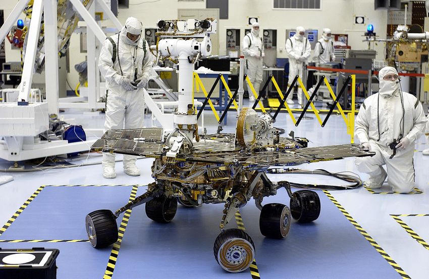
2.4 Spirit and Opportunity
In 2004 NASA launched two rovers named Spirit and Opportunity as part of the Mars Ex-
ploration Rover (MER) mission. The rover, shown in Figure 2.4, carried a 20 MHz RAD6000
CPU, a radiation hardened single board computer launched in 1997 capable of executing
35 million instructions per second (MIPS) [5]. The position estimation software on these
rovers leveraged an inertial measurement unit (IMU), wheel encoding, and a stereo cam-
era pair (Navcam). The IMU was a Litton LN-200 from Lockheed Martin with three-axis
accelerometers and three-axis angular rate sensors (gyroscopes). This IMU is an aerospace
grade device with extremely low drift (< 3◦ per hour), allowing for reliable attitude estima-
tion. The rover combined this attitude estimate with wheel encoding to estimate position
and orientation at a rate of 8 Hz [6].
Using the Navcam, the rover acquired a sequence of Navcam stereo pairs. These images
were processed along with the initial pose estimate from the encoders and IMU through
7Figure 2.2: Sojourner was the first rover to roam another planet. Similar to modern space
micro-rovers, the 11.5 kg rover was intended to operate only for a 7 day mission, drawing
power from its solar panel and non-rechargeable battery.
Figure 2.3: Sojourner’s computer vision system checked a set of fixed points for obstacles
along the projection of its light stripes. If a light stripe beam was not viewed at the predicted
location, an obstacle was assumed to be present and the navigation system responded
accordingly.
the use of visual odometry to create an improved estimate. Since the computer required
an average of nearly three minutes of computation time per visual odometry loop, vision
sensing was used primarily for short drives under 15 m where there was either high tilt
(> 10◦ ) or high slip. For the remaining part of the operation, the encoder and IMU were
used along with periodic attitude corrections based on imagery of the sun’s position. In test
8situations, the visual odometry algorithm and encoder with IMU both had similar results
for simple terrain, and visual odometry vastly outperformed the encoder with IMU system
for complex terrain with rough obstacles and high slip (under 2% absolute position error).
Figure 2.4: Spirit was the second rover to successfully reach Mars after Sojourner in 1997.
It was also one of the first mobile robots to rely on visual odometry for localization.
2.5 Curiosity
In August 2012, NASA’s Curiosity rover successfully landed on the Martian surface. The
rovers carried two identical computers, each of which use the RAD750 CPU, capable of
executing 400 MIPS, over 10 times more than Spirit and Opportunity. Curiosity, shown
in Figure 2.5, carried four pairs of black-and-white hazard avoidance cameras (Hazcams)
mounted on the lower portion on the front and rear of the rover. These cameras have a
field of view of 120◦ and map a region of the terrain 3 meters ahead and 4 meters across
the rover in 3D. These images allowed the rover to avoid obstacles and observe the nearby
terrain. The rover also carried two pairs of navigation cameras (Navcams). These cameras
were mounted on the mast of the rover and pointed towards the ground. They generated
panoramic imagery that complemented the views from the Hazcams. The rover also had
the same IMU as the MERs rovers and its localization algorithms were very similar to those
on the MERs mission. One interesting addition was the use of the Mars Reconnaissance
Orbiter (MRO), a spacecraft orbiting Mars, in capturing stereo images of the terrain with a
ground resolution of 0.3m. Images of the rover’s tracks were taken periodically as the MRO
flew over the landing side and used to determine rover position. The rover’s own Navcam
images and the images from the MRO were compared to determine the rover’s position [7].
9Figure 2.5: Curiosity’s selfie at the ’Mary Anning’ location on Mars was created by stitching
together images taken from a camera on the end of its robotic arm.
2.6 Yutu-1 Rover
In 2013 the China National Space Administration (CNSA) launched the Chang’e-3 system
to the lunar surface. This system carried a rover named Yutu, shown in Figure 2.6. Yutu
used a stereo camera pair mounted about 1.5 m above the ground. This camera was able
to be rotated in the yaw and pitch directions, allowing for the rover to capture multiple
regions from one location. Like the Spirit and Opportunity, the baseline localization system
of Yutu relied on using an inertial measurement unit and wheel encoder data. This system
was augmented by a visual odometry algorithm using sparse feature correspondences from
multiple images like in Spirit and Opportunity. The first step of the algorithm is searching
for feature correspondences across successive stereo image pairs, with search regions ini-
tialized by the baseline position estimator. The ASIFT method [8] is used to detect and
match these feature points. Initial 3D coordinates of these points are computed through
using stereo triangulation and using the initial pose estimates. The 3D points and the pose
estimate are then jointly optimized using a bundle adjustment procedure which minimizes
image reprojection error. Interestingly, these computations were done on Earth using images
transmitted from the rover, unlike the Mars rovers which were done on-board. Nonetheless,
the computed pose estimates played an important role throughout the Chang’e-3 mission.
In test scenarios, the baseline localization system reached an error of about 14%. The visual
odometry system was able to achieve an accuracy of about 5% for a 43 m path [9][10].
2.7 Pragyan
In 2019 the Indian Space Research Organization (ISRO) launched the Pragyan rover to the
moon. Unfortunately, the rover’s lander Vikram crash-landed on the lunar surface. Contact
with the rover and the lander was not possible after this incident. Very little is documented
about the rover’s autonomy software since ISRO only reports on successful missions. How-
ever, it publicly is known that the rover carried two 1 megapixel, monochromatic cameras
10Figure 2.6: Yutu-1 was China’s first lunar rover. Yutu-2, its successor, was launched in
2019.
[11]. The rover, shown in Figure 2.7, had a rocker-bogie suspension system and six wheels,
each driven by a brushless DC motor. Thus, wheel encoder data was likely available in the
form of the commutation of the motors. The rover’s processor was an Honeywell HX1750, a
radiation hardened microprocessor with a maximum clock rate of 40 MHz [12] and any ad-
vanced autonomy processing would have been done at the ground control station on Earth
after transmitting images. ISRO stated a digital elevation model was used by the ground
control team to aid in generating motion commands for the rover. Pragyan also carried
a sun sensor that was used in closed loop control to align the robot’s solar panels with
the sun to maximize solar charging. Compared to prior rovers, this system was relatively
primitive in its operation and capabilities. ISRO built their rover at a low cost for a higher
probability of success at the cost any on-board, real-time, and intelligent pose estimation
and autonomy.
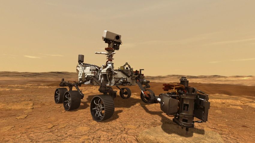
2.8 Perseverance
In February 2021, NASA’s Perseverance rover successfully landed on the Martian surface
as part of the Mars 2020 mission. The design of Perseverance, shown in Figure 2.8, was
based on that of Curiosity with different instruments and various improvements. The rover
carries the same computer as Curiosity, the RAD750. It has two Navcams mounted on its
mast, four Hazcams on the front, and two Hazcams on the rear [13]. As of this writing,
little has been publicly revealed of the specific localization algorithms on rover.
2.9 Conclusion
From the early 1970s to the 2020s, national space agencies from around the globe have pur-
sued the development of space rovers that can bring significant scientific, technological, and
11Figure 2.7: Pragyan carried a side mounted solar panel as it was headed to the southern
polar region of the moon.
Figure 2.8: Perseverence is the most sophisticated space rover to date, carrying numerous
scientific instruments used to study the Martian environment and sensors for navigation,
including a total of 23 cameras.
political return. All rovers were designed to be highly reliable, necessitating the use of radia-
tion hardened computing and as a consequence restricting their computational capabilities.
As a result, the majority of these rovers have been teleoperated by highly trained human
operators using visual feedback. Interestingly, all rovers, autonomous or teleoperated, have
relied on a similar baseline pose estimation system using wheel encoding, gyroscopes, and
accelerometers. Most have used sun sensing to correct their heading. In recent times, many
have leveraged visual odometry to deal with slip and rough terrain. These estimation sys-
tems have been proven to be accurate, allowing for multiple missions to successfully navigate
on the Moon and Mars. With much more to uncover in the vast universe, future rovers will
continue to rely on such systems as the backbone of their missions.
12Chapter 3
MoonRanger
3.1 Introduction
MoonRanger is a micro-rover built by Carnegie Mellon University’s Robotics Institute [14].
The rover is scheduled to reach the South Pole of the Moon in December 2022. Its purpose to
characterize hydrogenous volatiles while demonstrating autonomous micro-rover capabilities
during lunar polar exploration. Built on a shoe-string budget compared to prior space
robotics programs, it is part of a new class of space rovers that are only intended to survive
for a lunar day, or two Earth weeks. This short mission length enables the selection of
hardware that does not need to survive the extremely cold temperatures of lunar night. It
also precludes the need for expensive radiation hardened electronics designed to withstand
harsh radioactive environments.
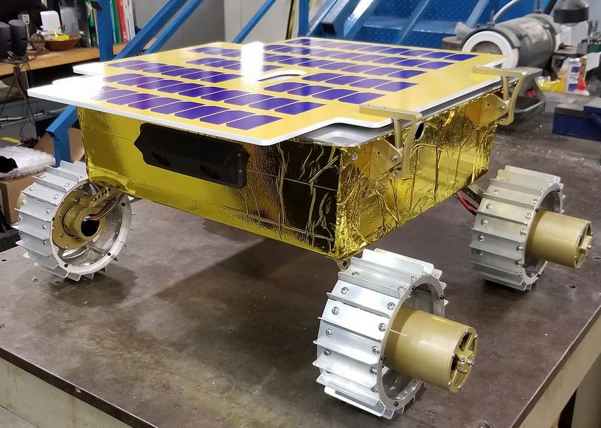
Figure 3.1: MoonRanger has a solar panel mounted on one side because of the low incident
angle on the lunar poles.
13This type of mission also necessitates complete autonomy, as a two week mission with slow
and careful teleoperation used in prior space rovers will not be able to achieve valuable
science return. Instead, the rover will need to accomplish high level objectives on its own.
This in turn necessitates the use of modern embedded computing solutions capable of state
of the art autonomy. The rover must reliably sense its position, map its environment, plan
obstacle free paths, drive autonomously, and transmit data; all in real time.
3.2 Avionics
The avionics architecture of the rover is shown in Figure 3.2. The rover’s main process-
ing unit is an Nvidia TX2i [15]. The TX2i carries a dual-core Denver 2 64-bit CPU and
quad-core ARM A57 Complex, as well as 256 GPU cores, enabling state of the art com-
puter vision algorithms to be run in real time. The TX2i is interfaced using a ConnectTech
Spacely carrier board [16]. To communicate with peripherals, a CubeSat microcontroller
from ISIS SPACE with flight heritage is used [17].
Because of budgetary, thermal, and weight constraints, the rover is fitted with a single
sided solar panel that faces outwards towards the sun, as shown in Figure 3.1. Thus, the
rover carries two pairs of stereo cameras, each on the front and rear side of the rover. The
sensor of the camera is the Sony IMX274 and the camera module itself is from Leopard
Imaging [18]. The rover’s inertial measurement unit is a STIM300 from Sensonor [19].
This IMU√ has flown on more than a hundred CubeSat missions and offers low gyro drift
(0.15◦ / h), making it suitable for a space rover. Each of the rover’s four brushless motors
provide wheel encoder data. Additionally, the rover has a Nano-SSOC-A60 analog sun sen-
sor mounted at the top of its solar panel to provide an absolute heading measurement [20].
The rover also carries light strip lasers and infrared dot projectors that can be used to map
its terrain in darkness to avoid obstacles [21].
3.3 Operation
In its mission, MoonRanger must complete a sequence of treks of increasing difficulty and
distance. The treks are predetermined based on the specified landing site and locations of
scientific interest. At the start of each trek, the rover is given a list of waypoints by the
mission operations team. The rover autonomously navigates to the targets autonomously
and logs data including current hydrogen content from its on-board Neutron Spectrometer
System (NSS) [22], its pose estimate, time, images, and other relevant telemetry. The rover
communicates to the lander via WiFi and is capable of traversing outside of the WiFi range
of the lander. At the end of each trek, the rover transmits the mission data to the lander
which forwards it to the ground control team on Earth.
Throughout its operation, MoonRanger must possess a reliable pose estimate to accurately
tag its NSS data in order to provide valuable science return and safely travel in and out
of the wireless communication range of the lander. The remainder of this thesis outlines
MoonRanger’s pose estimation algorithm that addresses this challenge.
14Figure 3.2: MoonRanger has numerous components that are commerical off-the-shelf or
custom made to save on cost.
15Chapter 4
A Baseline Position Estimator
4.1 Introduction
In this chapter we derive an Extended Kalman Filter (EKF) [23] that fuses accelerometer
and gyroscope data from an inertial measurement unit (IMU) to estimate orientation. This
orientation estimate is used with wheel encoder data to estimate position. Our work is
derived from [24].
4.2 Notation
In this EKF, we estimate the orientation, gyroscope bias, and accelerometer bias. We denote
our state with x:
x = [b, xg , xa ] (4.1)
In the above, b is the quaternion describing inertial to body frame transformation, xa is
accelerometer bias, and xg is gyroscope bias. An estimated variable will be denoted with
a hat, such as b̂. A sensor output with have a tilde above, such as ũ. A variable preceded
by a ∆, such as ∆f , denotes an error or difference. A variable with no tilde or hat denotes
the true value. The superscript − denotes the estimate before a measurement update and
+ denotes it after. The subscript k denotes the time tk , i.e., b(tk ) = bk . We assume our
global frame is our inertial frame, and denote the inertial frame by i and body frame by b.
We assume the body frame aligns with the IMU output frame, i.e., the IMU frame is at the
center of the rover. Also, we denote b in rotation matrix form as Rbi and its transpose Rib .
4.3 Extended Kalman Filter
We use an error-state EKF in our implementation [24]. A block diagram of the filter is
shown in Figure 4.1. In our implementation, the IMU’s gyroscope is integrated to estimate
orientation at 125 Hz. The rover’s accelerometer provides aperiodic corrections to the
orientation, gyroscope biases, and accelerometer biases using its predicted gravity vector
when the rover is stationary.
16Figure 4.1: Complementary Filter Block Diagram
4.4 IMU Sensor Model
Let u denote the gyroscope measurement. We denote wib b as the angular velocity of the body
with respect to the inertial frame, in the body frame. Then, the gyroscope measurement
model is
b
w̃ib = wib
b
+ xg + νg = wib
b
+ ∆wibb
(4.2)
where νg is Gaussian white noise with power spectral density (PSD) σν2g and xg is a bias
modeled as a first-order Gauss-Markov process:
ẋg = Fg xg + wg (4.3)
where Fg = −λg I and wg is a Gaussian white noise process with PSD σw 2 .
g
The accelerometer measures the specific force vector f b in the body frame. We denote Gb
as the gravitational acceleration vector in the body frame. Furthermore, we denote abib as
the acceleration of the body with respect to the inertial frame, measured in the body frame.
Then, the accelerometer measurement model is:
f˜b = f b + xa + νa = abib − Gb + xa + νa = f b + ∆f b (4.4)
where νa is Gaussian white noise with PSD σν2a and xa is a bias modeled as a first-order
Gauss-Markov process:
ẋa = Fa xa + wa (4.5)
where Fa = −λa I and wa is a Gaussian white noise process with PSD σw 2 .
a
Thus, given measurements w̃ibb and f˜b , the angular rate and specific force vectors for use in
the navigation equations are computed as
b
ŵib = w̃ib
b
− ∆ŵib
b
= w̃ib
b
− x̂g (4.6)
17fˆb = f˜b − ∆fˆb = f˜b − x̂a (4.7)
In practical applications, the PSD terms are derived after calibrating the IMU’s accelerom-
eter and gyroscope and analyzing its Allen Variance curves.
4.5 IMU Kinematic Model
In this section we derive the equations for computing the state estimate based on the
integration of sensor signals through the vehicle kinematics. The orientation update step
uses the angular velocity measurement from the gyroscope to update orientation. The
kinematic equation for the quaternion b representing rotation from the i frame to b frame
is
−b2 −b3 −b4
1 b b4 −b3
ḃ = 1
b
w
2 −b4 b1 b2 bi
b3 −b2 −b1
Thus, given an initial estimate of our orientation b̂(0) and ŵbib , we can integrate the above
equation to compute b̂(t). In discrete time, we represent our orientation at time-step k by
b(tk ), with ∆t as the time between time-steps.
From our sensor model, we have ŵib b = w̃ b − x̂ , and since ŵ b = −ŵ b , we have
ib g ib bi
b
ŵbi = x̂g − w̃ib
b
(4.8)
Then we can update our orientation estimate b̂(tk ) with the following equations [25]:
b ∆t
wbi b ∆t
wbi b
wbi
b̃k = [cos , sin ] (4.9)
2 2 b
wbi
b̂(tk+1 ) = b̃k b̂(tk ) (4.10)
4.6 EKF Prediction Update
In this section a state space model for our estimator is derived [24]. The general form of a
state space model used in an error-state EKF is
∆ẋ(t) = F (t)∆x(t) + G(t)w(t) (4.11)
where F is the state transition model and G is the noise transformation matrix, ∆x is the
state error vector with covariance P , and w is the noise vector with covariance Q. We now
derive these terms for our IMU. We define the error vector as
∆x = [ρ, δxg , δxa ] (4.12)
where, dropping superscripts denoting frames for clarity:
18• ρ is the orientation error: ρ = [x , y , z ]. ρ contains the small-angle rotations defined
in the inertial frame that aligns the true orientation with the estimated orientation.
• δxg is the gyroscope bias error vector: δxg = xg − x̂g .
• δxa is the accelerometer bias error vector: δxa = xa − x̂a .
We define the noise vector using the quantities from section 4.4
w = [νg , νa , wg , wa ] (4.13)
Substituting from the section 4.4, we compute
δf b = ∆f b − ∆fˆb = δxa + νa (4.14)
b
δwib = ∆wib
b
− ∆ŵib
b
= δxg + νg (4.15)
Now we compute the elements of F and G for our system.
ρ̇ = R̂ib δwib
b
= R̂ib δxg + R̂ib νg (4.16)
δ ẋa = ẋa − x̂˙ a = Fa δxa + wa (4.17)
δ ẋg = ẋg − x̂˙ g = Fg δxg + wg (4.18)
Putting the above in matrix form, where each element is 3x3, we have
0 −R̂ib 0
F = 0 Fg 0 (4.19)
0 0 Fa
−R̂ib 0 −R̂ib 0
G= 0 I 0 0 (4.20)
0 0 0 I
The estimator is assumed to be run at a fast enough rate such that all of the variables
above are constant between time steps, allowing continuous variables to be estimated using
discrete operations. From this model, we can compute the discrete state transition matrix
Φk ≈ eF ∆t (4.21)
The discrete process noise covariance matrix Qd at time step k is approximated as
Qdk = GQGT ∆t (4.22)
The covariance of the state at time step k can be updated according to
Pk+1 = Φk Pk ΦTk + Qdk (4.23)
194.7 EKF Measurement Update
To correct our orientation estimate, we use the gravity vector predicted from our orientation
and compare it to the known gravity vector Gi . We first derive the measurement matrix
that is used to compute the Kalman gain in the EKF following [24]. Subtracting biases,
the body frame estimate of gravity is
ĝ b = x̂a − ya (4.24)
The inertial frame estimate of gravity is then
ĝ i = Rib ĝ b (4.25)
The residual gravity measurement in the inertial frame is
δg i = g i − ĝ i (4.26)
Substituting the above, the measurement error
δg i = Ha δx + Rib νa (4.27)
can be described by the measurement matrix
h i
Ha = [−g i ×] 0 Rib (4.28)
The noise matrix of the current predicted gravity reading can be computed as Ra = Rib QRib
T.
Now we have all of the ingredients to compute the Kalman gain
K = P − HaT (Ra + Ha P − HaT )−1 (4.29)
Practically, this measurement update routine only works when the rover is still. Thus,
we detect if the rover is still if its acceleration is within a threshold close to zero for N
consecutive readings, or equivalently:
| fˆb − g| < k (4.30)
where k is some threshold, such as 0.1m/s2 . We set N as 250 for our application, so with
a 125 Hz IMU this test takes two seconds. We record all N accelerometer readings and
average these to obtain
ya = 1/N f˜ib (4.31)
X
i
Using this value and substituting into (4.24) and (4.25), we form our estimated gravity
vector ĝ i in the inertial frame and then compute the residual
z = ĝ i − Gi (4.32)
We substitute this residual in the EKF algorithm to compute our state correction δx+ =
[ρ, δxg , δxa ], and update our state by the following:
20• ρ is equivalent to a skew symmetric matrix representing small angle tilt errors. This
matrix can be represented as
0 −z y
P = [ρ×] = z 0 −x (4.33)
−y x 0
• We update the orientation with
(R̂bi )+ = (R̂bi )− (I − P ) (4.34)
We convert this back to quaternion form to obtain b̂+ .
• We update the biases:
(x̂g )+ = (x̂g )− + δxg (4.35)
(x̂a )+ = (x̂a )− + δxa (4.36)
• We update the covariance
P + = (I − KH)P − (4.37)
4.8 Wheel Encoding to Estimate Position
We now use the orientation estimate derived above and the wheel encoding of the rover to
update the rover’s position pk in the inertial frame. Each wheel rotates via a brushless DC
motor whose commutations are used as wheel encoder ticks. Each encoder tick is linearly
proportional to a fixed rotation angle of the corresponding wheel. In the estimator, the
encoder measurements are sampled at a fixed rate, with interval ∆t between samples. For
MoonRanger, the encoder sampling rate is about 10 Hz. Thus, given encoder ticks between
each time step ∆t, each wheel i turns ∆θi radians and travels ∆di = R∆θi distance where
R is the radius of the wheels. The distance traveled by the rover in a time step is estimated
as
1X
∆d = ∆di . (4.38)
4 i
Thus, interpolating the orientation at the beginning of the time step bk and at the end
bk+1 and denoting the inverse of this rotation as q, we can update position via a quaternion
rotation according to
pk+1 = pk + q(∆d)q −1 (4.39)
Finally, at each time tk we have an estimate of orientation bk and position pk .
4.9 Initialization
Before driving the rover, we must compute its initial orientation b0 [24]. Assuming aib = 0
and xa = 0, the estimate of the body frame gravity vector is computed by averaging
accelerometer measurements
1 T ˜b
Z
g̃ b = −f (τ ) dτ (4.40)
T 0
21The roll and pitch angles are computed as
φ̂(T ) = atan2(g̃2 , g̃3 ) (4.41)
q
θ̂(T ) = atan2(−g̃1 , g̃22 + g̃32 ) (4.42)
The roll and pitch are then used to compute the rotation matrix of the body Rib , and this
is inverted and converted to quaternion form b. Without an absolute heading estimate, we
initialize yaw as 0. However, as discussed in the next chapter, we can use the sun sensor
to initialize our heading. Furthermore, [24] can be referenced for a comprehensive way to
initialize covariances.
4.10 Gravity on the Moon
One key difference between this algorithm running on Earth and on the Moon is the value
of the gravitational constant. With a rough knowledge of the landing site, this value can be
predetermined using existing gravity field models as shown in Figure 4.2 of the lunar surface
[26]. Furthermore, many algorithms take into account the rotation of the celestial body for
higher fidelity models of the dynamics. These terms were neglected in our implementation.
Figure 4.2: The estimated acceleration due to gravity on the lunar surface ranges from
1.611m/s2 to 1.636m/s2 [26]
22Chapter 5
Sun Sensing
5.1 Introduction
In this chapter, MoonRanger’s sun sensing algorithm will be described. The primary issue of
relying on the IMU’s gyroscope is that there is no absolute correction, since the measurement
update step of the EKF only corrects roll and pitch. Thus, over time, the rover’s heading
estimate will drift as error is integrated. This is especially dangerous for longer drives.
Assuming the lander wireless range is 100 m and the rover takes a U-turn at the end of a
1km trek, an accumulated error greater than 6◦ will steer the rover outside of the comm
range upon its return. MoonRanger carries a nanoSSOC-A60 sun sensor [20] mounted on
top of its solar panel. As shown in Figure 4.1, the sensor provides a field of view of 120◦ .
Figure 5.1: Given MoonRanger’s one sided solar panel configuration, its sun sensor faces
towards the sun for the entire duration of the drive
The sensor provides an accuracy of < 0.5◦ and a precision of < 0.1◦ . Thus, it is capable of
providing a reliable heading correction throughout the rover’s mission. The sensor outputs
two angles that describe the incident sun ray relative to its own coordinate system, as
visualized in Figure 4.2.
23Figure 5.2: The incident sun ray vector can be computed from the angles from the sensor
[20].
5.2 Procedure
The sun sensor’s output angles α and β can be used to determine a ray to the sun v in
the sun sensor’s frame s. Using the engineering drawings of the system, the rotation to the
body frame of the rover can be determined Rbs . Thus we first compute the sensor’s reading
in the body frame [27]:
ṽb = Rbs ṽs (5.1)
The next step is to predict the sun ray in the inertial frame using the current orientation
estimate:
v̂i = R̂ib ṽb (5.2)
Using ephemeris data, such as via [28], we can determine the true sun ray as a function of
time vi . We assume that the spatial variation in the rover’s position is not significant and
so can use the data for a single location, such as the landing site. Based on the analysis in
[24], we can form a measurement matrix as
h i
Hs = −[vi ×] 0 0 (5.3)
24where [vi ×] is the skew symmetric representation of the true sun ray. We assume the sun
ray outputs two angles α and β each with noise σs and denote compute a noise matrix as
" #
σ 0
Rs = s (5.4)
0 σs
Using the function vs = f (α, β), we compute its Jacobian J and transform the noise into
the inertial frame:
Rs = R̂ib Rbs JRs J T Rbs
T T
R̂ib (5.5)
We can finally substitute these values into our EKF measurement update step following
section 4.7 to correct our state estimate. With this addition, the roll, pitch, and yaw of the
rover are all corrected throughout the rover’s mission. Furthermore, we can initialize our
heading of the rover using the output of this procedure.
25Chapter 6
Visual Odometry
6.1 Introduction
In this chapter, MoonRanger’s visual odometry algorithm will be described. One problem
of the pose estimator described so far is the complete reliance on wheel encoders to update
position. There are numerous scenarios where this baseline system would fail. For example,
if the robot slips, which is a common occurrence on soft soils and sloped terrains, the
position estimate will have traveled a larger estimate than in reality. Another example is
when the rover drops over a rock; the position estimate has no way to detect the change
in height. The baseline estimate assumes no slip and having the rover in contact with the
ground at all times, an unrealistic assumption. A system that solves this issue is the use
of visual odometry [6][29][30]. Through the tracking of visual features in the terrain, the
system is robust against slip and suddenly dropping motions. We base our implementation
on [31].
6.2 Feature Detection and Matching
The visual odometry pipeline receives rectified stereo images at 2 Hz facing the rover’s
direction of motion, as shown in Figure 6.31. After obtaining the first set of images, I0l and
Figure 6.1: An image from MoonRanger’s stereo cameras in a lab setting.
I0r , where 0 denotes the image number, l denotes the left image, and r denotes the right
26image, the FAST feature detector [32] is run on the left image to obtain an initial list of
features. The image is partitioned into evenly spaced buckets where up to 5 features per
bucket is selected. The most stable features are selected by using a weighted function of
their age and strength. This enables an even distribution of feature points across the image
and reduces the probability of false matches, as shown in Figure 6.2.
Then the next pair of stereo images, I1l and I1r are received. Using the a sparse iterative
Figure 6.2: Feature points before and after bucketing.
version of the Lucas-Kanade optical flow using pyramids [33][34], the features from I01 are
matched in I0r , the matched features from I0r are matched in I1r , the matched features in
I1r are matched in I1l , and finally the matched features in I1l are matched back into I0l .
This procedure is called circular matching, coined by [31]. As a result, feature points that
are present in all four images are available as shown in Figure 6.3.
Figure 6.3: Feature matches between the subsequent images.
This procedure effectively eliminates false matches between image sequences and is a key
benefit of using stereo cameras.
276.3 Motion Estimation
Labelling the matched feature points in the first stereo pair as p0l and p0r , we can use
stereo triangulation to find their 3D coordinates. These coordinates are relative to the
rover’s camera frame at the instant I0l and I0r were captured. Labelling the corresponding
matched features in the second left image as p1l , we can employ the Perspective-n-Point
(PnP) method with RANSAC [35] to compute the rotation and translation between image
sequences. These are relative to the camera’s reference frame and can be converted to the
rover’s body frame using a pre-calibrated camera to body frame transformation. We denote
the translation change between image sequences as ti,i+1 . Furthermore, these rotations and
translations can be accrued for each new stereo pair of images, forming a pose estimate
update for every image sequence.
6.4 GPU Utilization
All of the stages of the pipeline were chosen to leverage the TX2i’s 256 CUDA GPU cores.
We use the GPU version of the fast feature detector, circular matching, and PnP algorithms.
We leverage the use of existing libraries from [36] for the majority of these functions.
28Chapter 7
System Design and Testing
7.1 System Design
Throughout MoonRanger’s treks, the rover will encounter a variety of scenarios that affect
the performance of each of the techniques described above. The baseline system will fail
when the rover’s wheels slip in the sand, overestimating the distance travelled. The visual
odometry system will fail in regions of complete darkness and on featureless terrain. The
sun sensor will fail when there is no incident sun ray, such as when the rover is facing away
from the sun. It is the challenge for the team to engineer a solution that can make the best
use of each subsystem when possible.
A high level overview of the proposed system is shown in Figure 7.1. When visual odometry
and sun sensing is not available, MoonRanger will rely on the baseline position estimator
from Chapter 4. When sun sensing is available, the orientation estimation EKF will use
it for measurement updates to correct heading. When visual odometry is available, Moon-
Ranger will use its estimated translation in place of the wheel encoding. Since it relies only
on the current and previous set of stereo images, it is amenable to being used aperiodically.
The entire system working together is named the integrated system.
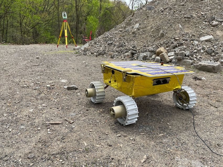
7.2 Testing
To test MoonRanger’s pose estimation algorithms, a prototype rover was built to emulate
the rover’s dimensions and sensing capabilities, as shown in Figure 7.2. The rover carries
the same cameras and IMU as MoonRanger and is driven by brushed DC motors rather
than MoonRanger’s brushless motors. The space-rated sun sensor was not available for use
and so the sun sensing component of the system was not considered in testing.
To quantify our algorithm’s performance, we use the 2D Absolute Trajectory Error (ATE)
metric as discussed in [37]:
−1
1 NX
AT E pos = ( k∆pi k)2 (7.1)
N i=0
Since MoonRanger will return to its start location after each of its treks, the rover was
29Figure 7.1: MoonRanger can always rely on its IMU and wheel encoding as a fallback. The
sun sensor and visual odometry may be unavailable at times.
Figure 7.2: MoonRanger’s surrogate rover used to test pose estimation algorithms.
driven in a loop back to its final location during the tests. We are interested in the absolute
30error of the final position, or Final Position Error (FPE):
F P E = k∆pN k (7.2)
During the mission the wireless communication range to the lander can be assumed to be
80 meters. Therefore, an FPE under 5% allows a trek distance up to 1600 m to be driven by
the rover reliably. In our experiments, the ground truth position of the rover was measured
using a surveying instrument. A reflective marker was fixed onto the rover and was tracked
with sub-mm accuracy at a rate of 7 Hz.
The rover was first tested in an indoor setting with rubber wheels. The rover was driven a
total distance of 40 m in a swerving manner. The ground was a smooth polished surface that
caused the rover to slip considerably and precluded the use of visual odometry. Figures 7.3
and 7.4 show the baseline system’s position estimate and the ground truth measurement in
the x and y dimensions versus time, respectively. Figure 7.5 shows the 2D plot of the rover’s
estimated and true path. As can be seen in the figures, the rover’s estimate using only the
baseline system performs well for this benign environment with an AT E pos = 0.4614 m and
F P E = 0.5247 m. This leads to a position final error under 5%, which is suitable for the
MoonRanger mission requirements.
In the next test the rover was taken to a lunar analogue site and fitted with MoonRanger-like
wheels, as shown in Figure 7.6. The surface was compact and rocky, causing grinding and
skidding during the rover’s turns. In this test, the ground truth position was again tracked
using the surveying instrument. The rover was driven a total distance of 50 m. The baseline
and integrated system position was recorded. Figures 7.7 and 7.8 show the baseline system
and integrated system’s position estimate along with ground truth measurement in the x
and y dimensions versus time, respectively. Figure 7.9 shows the 2D plot of the rover’s
estimated and true path. The rover’s estimate using only the baseline system performs
slightly poorer than in the previous test with an AT E pos = 0.4724 m and F P E = 0.4737
m. The integrated system performs slightly worse than this with an AT E pos = 0.5493 m
and F P E = 1.0961 m. Again, this leads to a final error under 5% for both techniques. We
can be confident that these algorithms, without the benefit of heading corrections from the
sun sensor, can provide adequate localization for MoonRanger.
31Figure 7.3: Position in the X coordinate versus time (indoor test).
32Figure 7.4: Position in the Y coordinate versus time (indoor test).
Figure 7.5: The X-Y position of the rover (indoor test).
33Figure 7.6: The surrogate rover being tracked by the surveying instrument in the outdoor
test.
34Figure 7.7: Position in the X coordinate versus time (outdoor test).
35Figure 7.8: Position in the Y coordinate versus time (outdoor test).
Figure 7.9: The X-Y position of the rover (outdoor test).
36Chapter 8
Conclusion
In this thesis we analyzed the space rovers of the past and developed the motivation for
MoonRanger’s sensing, avionics, and pose estimation algorithms. We derived all steps of
MoonRanger’s pose estimation pipeline, including the use of wheel encoding, an inertial
measurement unit, and a stereo camera. We evaluated the results of these algorithms
on two testing locations and quantified their accuracy against ground truth position mea-
surements. We concluded that our algorithms provide a final position error of under 5%,
matching the performance of the space rovers of the past. This gives us confidence that
MoonRanger will be able to accurately map the NSS data along its trek and will be able
to navigate in and out of the communication range to the lander. The proposed system
is lightweight and the most computationally challenging components leverage the Nvidia
TX2’s GPU, leaving sufficient computing resources for other mission critical processes.
In the near future the rover will be tested in various conditions to improve the pose es-
timator’s reliability. These tests include sloped sand pits where the rover’s will skid in its
direction of travel, as shown in Figure 8.1. This environment will likely cause the base-
line system to overestimate distance travelled and will highlight the importance of visual
odometry. Furthermore, the rover will be outfitted with its flight motors and be gravity
offloaded to match the true flight mechanical specifications. The sun sensor will be tested
on a benchtop to verify its accuracy as part of the orientation estimation pipeline. A solar
ephemeris model will be developed to predict the movement of the sun for the MoonRanger
mission. Various tests will be conducted to quantify the sensitivity of the system to sensor
failure and changing environmental conditions, such as temperature. These tests will lead
to a position estimator capable of operation on the challenging environment of the Moon,
enabling MoonRanger to achieve all of its mission requirements. We make all of our software
is publicly available [38][39] for others to benefit from our efforts.
37Figure 8.1: A MoonRanger surrogate climbing a sloped surface.
38References
1: Li, S., Lucey, P. G., Milliken, R. E., Hayne, P. O., Fisher, E., Williams, J. P., ... & El-
phic, R. C. (2018). Direct evidence of surface exposed water ice in the lunar polar regions.
Proceedings of the National Academy of Sciences, 115(36), 8907-8912.
2: NASA. Available at: https://www.nasa.gov/press-release/nasa-awards-contract-to-deliver-
science-tech-to-moon-ahead-of-human-missions
3: Kassel, Simon. Lunokhod-1 Soviet lunar surface vehicle. RAND CORP SANTA MON-
ICA CA, 1971.
4: https://mars.nasa.gov/MPF/rover/faqs sojourner.html#cpu
5: https://mars.nasa.gov/mer/mission/technology/
6: Maimone, Mark, Yang Cheng, and Larry Matthies. ”Two years of visual odometry on
the mars exploration rovers.” Journal of Field Robotics 24.3 (2007): 169-186.
7: https://mars.nasa.gov/msl/spacecraft/rover/cameras/
8: Morel, Jean-Michel, and Guoshen Yu. ”ASIFT: A new framework for fully affine invari-
ant image comparison.” SIAM journal on imaging sciences 2.2 (2009): 438-469.
9: Wan, W., Liu, Z., Di, K., Wang, B., & Zhou, J. (2014). A cross-site visual localization
method for Yutu rover. The International Archives of Photogrammetry, Remote Sensing
and Spatial Information Sciences, 40(4), 279.
10: Li, M., Sun, Z., Liu, S., Ma, Y., Ma, H., Sun, C., & Jia, Y. (2016). Stereo vision
technologies for China’s lunar rover exploration mission. International Journal of Robotics
and Automation, 31(2), 128-136.
11: https://www.isro.gov.in/chandrayaan2-spacecraft
12: Disclosed by sources wishing to remain anonymous
13: https://mars.nasa.gov/mars2020/spacecraft/rover/cameras/#Lander-Vision-System-Camera
14: https://www.nasa.gov/press-release/nasa-selects-12-new-lunar-science-technology-investigations
15: https://developer.nvidia.com/embedded/jetson-tx2i
16: https://connecttech.com/product/spacely-carrier-nvidia-jetson-tx2-jetson-tx1/
17: https://www.isispace.nl/product/on-board-computer/
18: https://www.leopardimaging.com/product/csi-2-mipi-modules-i-pex/csi-2-mipi-modules/rolling-
shutter-mipi-cameras/8-49mp-imx274/li-imx274-mipi-cs/
19: https://www.sensonor.com/products/inertial-measurement-units/stim300/
20: https://www.cubesatshop.com/product/nano-ssoc-a60-analog-sun-sensor/
21: Jamal, H., Gupta, V., Khera, N., Vijayarangan, S., Wettergreen, D. S., & Red, W. L.
(2020). Terrain Mapping and Pose Estimation for Polar Shadowed Regions of the Moon.
iSAIRAS, Virtual, October.
22: https://www.nasa.gov/image-feature/ames/the-neutron-spectrometer-system-nss
3923: Smith, Gerald L., Stanley F. Schmidt, and Leonard A. McGee. Application of statisti-
cal filter theory to the optimal estimation of position and velocity on board a circumlunar
vehicle. National Aeronautics and Space Administration, 1962.
24: Farrell, J. (2008). Aided navigation: GPS with high rate sensors. McGraw-Hill, Inc..
25: Whitmore, S.A., Hughes, L.: Calif: Closed-form Integrator for the Quaternion (Euler
Angle) Kinematics Equations, USpatent (2000)
26: Hirt, C., & Featherstone, W. E. (2012). A 1.5 km-resolution gravity field model of the
Moon. Earth and Planetary Science Letters, 329, 22-30.
27: Boirum, Curtis. ”Improving Localization of Planetary Rovers with Absolute Bearing
by Continuously Tracking the Sun.” (2015).
28: Acton, C., Bachman, N., Diaz Del Rio, J., Semenov, B., Wright, E., & Yamamoto, Y.
(2011, October). Spice: A means for determining observation geometry. In EPSC–DPS
Joint Meeting.
29: Nistér, David, Oleg Naroditsky, and James Bergen. ”Visual odometry.” Proceedings of
the 2004 IEEE Computer Society Conference on Computer Vision and Pattern Recognition,
2004. CVPR 2004.. Vol. 1. Ieee, 2004.
30: Scaramuzza, Davide, and Friedrich Fraundorfer. ”Visual odometry [tutorial].” IEEE
robotics & automation magazine 18.4 (2011): 80-92.
31: Cvišić, I., Ćesić, J., Marković, I., & Petrović, I. (2018). SOFT-SLAM: Computationally
efficient stereo visual simultaneous localization and mapping for autonomous unmanned
aerial vehicles. Journal of field robotics, 35(4), 578-595.
32: Rosten, Edward, and Tom Drummond. ”Machine learning for high-speed corner detec-
tion.” European conference on computer vision. Springer, Berlin, Heidelberg, 2006.
33: Lucas, Bruce D., and Takeo Kanade. ”An iterative image registration technique with
an application to stereo vision.” 1981.
34: Bouguet, Jean-Yves. ”Pyramidal implementation of the affine lucas kanade feature
tracker description of the algorithm.” Intel corporation 5.1-10 (2001): 4.
35: Fischler, Martin A., and Robert C. Bolles. ”Random sample consensus: a paradigm for
model fitting with applications to image analysis and automated cartography.” Communi-
cations of the ACM 24.6 (1981): 381-395.
36: Bradski, Gary, and Adrian Kaehler. Learning OpenCV: Computer vision with the
OpenCV library. ” O’Reilly Media, Inc.”, 2008.
37: Zhang, Zichao, and Davide Scaramuzza. ”A tutorial on quantitative trajectory evalua-
tion for visual (-inertial) odometry.” 2018 IEEE/RSJ International Conference on Intelligent
Robots and Systems (IROS). IEEE, 2018.
38: https://github.com/hjamal3/imu ekf ros
39: https://github.com/hjamal3/stereo visual odometry
40You can also read