Localization and panning of musical sources within the context of a musical mix - Alice Backlund

Localization and panning
 of musical sources within
the context of a musical mix

 Alice Backlund

 Audio Technology, bachelor's level
 2022

 Luleå University of Technology
 Department of Social Sciences, Technology and Arts

Alice Backlund
2022

Abstract
In recent years, the research on the localization of audio objects within a stereo context has
started to include musical audio objects. This study seeks to explore a research gap:
localization ability whilst hearing multiple sounds. This study aims to investigate listeners’
ability to localize panned musical audio objects within a musical context. Subjects listened to
two different versions of the same mix and were asked to simultaneously pan musical audio
objects with different characteristics. When comparing the results from the different mixes,
both mixes gave similar results. Therefore, the differences between the mixes had no impact
on localization accuracy. Additionally, this study was able to reconstruct previous findings
indicating that localization blur affects localization accuracy of wide-panned audio objects.

 1

Alice Backlund
2022

Acknowledgements
I would like to thank Jon Allan for his supervision during this project, as well as helping me
with calculations for the listening test. I would also like to thank Nyssim Lefford for her
assistance and guidance during the investigate phase of this project. A big thank you to Louise
Backlund for helping me proofread the essay and thank you to all of the participants of the
listening test.

 2

Alice Backlund
2022
Table of Contents
ABSTRACT .............................................................................................................................................................1
ACKNOWLEDGEMENTS ...................................................................................................................................2
1. INTRODUCTION .........................................................................................................................................4
 1.1 SPATIAL PERCEPTION ...................................................................................................................................4
 1.2 PANNING.........................................................................................................................................................5
 1.3 PRIOR RESEARCH ON PANNING AND PERCEPTION ......................................................................................6
 1.4 RESEARCH QUESTION & PURPOSE ...............................................................................................................8
2. METHOD .......................................................................................................................................................9
 2.1 CALCULATIONS OF PANNING ANGLES ..........................................................................................................9
 2.2 STIMULI ..........................................................................................................................................................9
 2.3 EQUIPMENT ..................................................................................................................................................10
 2.4 PARTICIPANTS..............................................................................................................................................11
 2.5 PROCEDURE .................................................................................................................................................11
 2.5.1 Task Procedure.....................................................................................................................................11
 2.5.2 S3 Control Surface ...............................................................................................................................11
 2.5.3 Pro Tools sessions ................................................................................................................................12
 2.6 TESTING OF DATA........................................................................................................................................12
3. RESULTS & ANALYSIS ...........................................................................................................................13
 3.1 PANNING DEVIATION ...................................................................................................................................13
 3.2 MEAN VALUE AND STANDARD DEVIATION ................................................................................................13
 3.3 CATEGORY RESULTS ...................................................................................................................................14
 3.4 T-TEST AND F-TEST ......................................................................................................................................17
4. DISCUSSION...............................................................................................................................................18
 4.1 ANGLES ........................................................................................................................................................18
 4.2 INSTRUMENT ................................................................................................................................................19
 4.3 MIX ...............................................................................................................................................................19
 4.4 PANNING SIDE ..............................................................................................................................................19
 4.5 CRITIQUE OF METHOD ................................................................................................................................20
 4.6 FINDINGS AND FUTURE APPLICATIONS ......................................................................................................20
5. REFERENCES ............................................................................................................................................22
6. APPENDIX A ..............................................................................................................................................23

 3

Alice Backlund
2022

 1. Introduction
This study regards the localization of stereo panned audio objects, an area of study that is
based in psychoacoustics and spatial perception. The positioning and localization of musical
and non-musical sources in a stereo sound setup have been researched since the 1920s,
generally focusing on panning laws and techniques as well as the difference in perception
regarding frequency content (Blauert, 1997). In the present study, the scope is narrowed down
to the localization of horizontally panned sources in a stereo context aimed for loudspeakers.

How localization in a stereo context works is an area of interest within the audio community
since the stereo listening experience is dependent on how the brain interprets the sound that
has reached each ear (Blauert, 1997). To perceive that a sound source is at a specific location,
there needs to be a difference in the localization information in each ear, namely in frequency,
time, and amplitude (Izhaki, 2012). When hearing a sound that is reproduced in stereo, it is
referred to as a virtual sound source. A virtual sound source refers to a audio object whose
position is created through the summation of the sounds projected from each loudspeaker,
whereas a non-virtual sound source is emitted from
one sound source alone.

This study aims to further the research of
localization, looking at how listening to multiple
sound sources might affect localization ability.
Previous research has mainly studied the accuracy of
different panning laws through listening to and
localizing one sound source at a time. Even though
these studies have brought findings that increased
knowledge in understanding what affects
localization, another part that makes human hearing
complex stills stands – oftentimes multiple sounds
are heard at a time and that is why this study aims to
further explore further this research area.

1.1 Spatial Perception Figure 1 - Recreated from Pulkki & Karjalainen, 2001,
To discuss the localization of sources in a stereo Fig 1. “Standard stereophonic listening configuration”,
 p. 741
sound field, one needs to understand the basics of
human auditory spatial perception. To localize any sound source, humans decode the
differences between the sound reaching the two ears. These differences can be divided into
temporal and spectral differences, in the field of perceptual audio more commonly known as
interaural time difference (ITD) and interaural level difference (ILD) (Pulkki, Lokki, 2011).
These are collectively called binaural cues/differences. It is possible to detect these
differences because of the separation between the two ears, the shape of the outer ear (pinna),
and the acoustic shadow of the human head and body. A sound will travel to each ear
differently depending on which direction the sound is coming from; this binaural information
of a sound is what provides the brain with directional information (Pulkki et al., 2011). The
spectral changes of a sound that are induced by the pinna and torso do not occur over the
entire frequency spectrum. According to Pulkki et al. (2011), the spectral changes of a sound
entering the ear canal are introduced above 1-2 kHz. Therefore, Pulkki et al. (2011) note that
if a signal has a too narrow bandwidth, these spectral cues cannot be decoded and the ability
of localization is therefore dependent on the spectrum of the signal.

 4

Alice Backlund
2022
Despite the sophisticated workings of human
hearing, localization is not always correct. For
example, there is a “cone of confusion” (Figure
2), which is an area where all points could be
confounded with each other. The sound source
may be wrongly identified within the cone, where
front-facing sounds are confused with back-facing
sounds and vice versa, as the difference in
distance to a source in the cone to each ear
remains the same (Pulkki & Karjalainen, 2001).
Pulkki and Karjalainen (2001) define the
placement and shape as being approximated “by a
cone having its axis of symmetry along a line
passing through the listener’s ears” (p. 740). To
improve the perceived direction of a sound within Figure 2 - Recreated from Pulkki et al., 2011, figure 5.1 p. 141
the cone of confusion, other mechanisms that also are a part of the localization process can be
used. These mechanisms could be such as the above-mentioned ITD and ILD cues provided
by the outer ear and torso of the listener, as well as head movements (Pulkki et al., 2011).

1.2 Panning
Panning works because listeners can detect level differences between the sounds arriving at
each ear. Izhaki (2012) explains that the illusion or effect of panning, a sound present in a
specific place in the stereo sound field (a phantom sound image), comes from having a sound
source’s level be different between the left and right channel. The modern panning
potentiometer works by splitting the signal to left and right and into its own gain control,
which controls the attenuation on one of the channels (Izhaki, 2012). This is commonly
known as “amplitude panning”, as it is the level of the sound that creates the effect. There are
other forms of panning, but amplitude-panning will be the method that will be the focus of
this study.

Music mixing frequently utilizes panning techniques to place and separate musical sources. In
addition to the placement, panning has other additional effects on sound sources. When two
objects who are panned to different sides are summed acoustically, their definition increases
because of the separation that panning provides (Izhaki, 2012). In addition, panning
instruments to the sides can also lead to an apparent loudness increase. Furthermore, one can
notice that most masking occurs in the central area when listening to two loudspeakers
(Izhaki, 2012). Izhaki (2012) elaborates;

 the center of the mix is the least-focused area (due to the late arrival of sound
 from both speakers to the respective far ear), while the extremes provide the
 most-focused area (as only one speaker generates the sound in true mono). (p.
 197).

This results in objects panned to the extremes being perceived as being closer to the listener
and having more definition and focus than the center-panned objects (Izhaki, 2012). When
regarding that panned objects are not as affected by masking as center-image audio objects,
and since this study seeks to explore the possibilities of locating audio objects whilst listening
to a mix, there is an indication that it is possible to locate sounds within a mix as compared to
one audio object at a time.

When practically implementing panning, the “panning law” is to be considered. A panning
law compensates for a sound’s perceived loudness in stereo versus in mono (Izhaki, 2012).
 5

Alice Backlund
2022
According to Izhaki (2012), when choosing a panning law there are two main principles to
consider. Firstly, when a signal with the same level is emitted from two loudspeakers, e.g. the
doubling of a signal, the perceived loudness will increase by 3 dB (Izhaki, 2012). Secondly,
the other principle concerns how mono is accomplished – half of the level of the two stereo
channels are sent to both left and right. Practically speaking, since this is a “halving” of the
level, this results in a 6 dB attenuation (Izhaki, 2012).

To further explain these principles, when implementing the second principle, if a hard-panned
signal is summed to mono the sound will be lowered by -6 dB. However, because of the first
principle, the perception of the sound is also increased by 3 dB since the sound is now
perceived as being equally loud from each loudspeaker. The result of this is that a hard-
panned signal played in mono will be perceived as 3 dB lower, whilst the center image
remains the same (Izhaki, 2012). As previously stated, a pan law compensates for how a
sound is perceived when summed to mono, to compensate for the 3 dB center boost (Izhaki,
2012). Izhaki (2012) therefore concludes that the -3 dB panning law is generally the best
option when mixing in stereo, as the signals remain at the same level when panned and thusly
do not require later level adjustments. Besides the -3dB panning law, other common panning
laws are 0, -4.5, and -6 dB.

The above-mentioned panning law is derived from theoretical sine- or tangent panning laws.
The sine law was first created by von Hornbostel and Wertheimer in 1920 (in Blauert, 1997).
Their formula regards the ears as two points in free space, separated by 21 cm and does not
calculate the shadowing effect of the human head (Blauert, 1997). As Blauert (1997) points
out, 21 cm is not an accurate depiction of the actual distance between the ears, the sine law
was thus later corrected.

Another more recent panning law was made by Bennett, Barker, and Edeko (1985, in Pulkki
et al. 2011), called the tangent law. Lee (2017) notes that the main difference between the sine
and tangent law is that the tangent law takes the listener’s head rotation into account. The
equation for the tangent law is presented below, where qT is the perceived angle and q0 is the
loudspeaker base angle, and g1 regards amplitude for the left channel and g2 for the right
channel respectively (Pulkki & Karjalainen, 2001).

 tan ! # − $
 =
 tan " # + $
 Equation 1 – Tangent Law

1.3 Prior Research on Panning and Perception
Pulkki and Karjalainen (2001) conducted a listening test where the localization of amplitude-
panned virtual sources in a stereophonic setting was investigated. Subjects listened to both
one-third-octave band filtered noise and two-octave-band noise (with several different types
of noise) and were asked to adjust the direction of a virtual source to correspond most
accurately to a real reference source (Pulkki & Karjalainen, 2001). This was made possible by
having two loudspeakers produce the amplitude-panned virtual source and another single
loudspeaker produce the real acoustic reference point (Pulkki & Karjalainen, 2001).

The horizontal location of amplitude-panned virtual sources was found to depend on both
ITD, ILD, and main directional cues and being dependent on frequency (Pulkki &
Karjalainen, 2001). The authors state that this could be why a single source with a broad-band
signal may be localized to multiple directions. The ITDs of amplitude-panned virtual sources
behaved consistently below 1100 Hz, and Pulkki and Karjalainen (2001) also point out that

 6

Alice Backlund
2022
their results show that the localization of amplitude-panned virtual sources is based on ITD
cues at low frequencies and ILD cues at high frequencies. Which cue that is most prominent
is dependent on its temporal structure, which might be why signals with the same magnitude
spectrum but different temporal structures were localized differently in Pulkki and
Karjalainen’s (2001) results. They continue:

 The coincidence of low-frequency ITD cues and high-frequency ILD cues
 explains why amplitude-panned virtual sources are localized fairly consistently
 across the audible spectral range. Therefore the sine and tangent laws that were
 derived using low-frequency ITDs hold also at high frequencies. However, the
 deviations of cues at middle frequencies may produce the spreading of virtual
 sources. (Pulkki & Karjalainen, 2001, p. 750)

In addition, Pulkki and Karjalainen (2001) note that natural signals such as vocal sounds and
musical instruments are broadband and thus also include frequencies below 1100 Hz. The
localization of the natural signals is therefore defined mostly by high-frequency ILDs and
low-frequency ITDs and could be localized rather accurately (Pulkki & Karjalainen, 2001).
However, if the virtual source contains frequencies only above 1100 Hz, the ITD cues of the
amplitude-panned (virtual) source will no longer aid in localization, resulting in the perceived
direction of the virtual source to spread out, as it will be mostly based on ILD cues (Pulkki &
Karjalainen, 2001).

Lee and Rumsey (2013) investigated the localization of musical objects, with the purpose of
testing the accuracy of different panning laws. The panning methods in question were based
on Interchannel Time- or Level Difference, ICTD and ICLD respectively. Pointing to the lack
of knowledge on the perceptions of panned musical instruments, the authors found little
previous research where musical sources had been used (Lee & Rumsey, 2013). Other
motivations for using musical sources were that musical sources have a more complex
envelope and harmonic nature (as opposed to noise or sinusoids), and are widely used in the
context of panning, as well as being considered more ecologically valid regarding ICLD and
ICTD panning values from musical sources (Lee & Rumsey, 2013). Due to this, a listening
test was conducted using musical notes where the influences of ICLD and ICTD on the
localization of stereo phantom images were investigated (Lee & Rumsey, 2013). The musical
sources used in the listening test were staccato piano at C2 and C6, trumpet at Bflat3 and
Bflat 5, as well as male speech (Lee & Rumsey, 2013).

The most important finding of Lee and Rumsey’s (2013) study was that it was easier for the
subjects to place sounds that were located at a smaller angle than at a larger one, with the 30°
panning angle (from the centerline) being especially difficult since the directional resolution
became lower around 20° (Lee & Rumsey, 2013). When comparing their results with
previous research, Lee and Rumsey (2013) remark that as the sound source moved from the
front towards the sides of the listener, the smallest change of a sound source that can be
detected, the minimum audible angle (MAA), became larger. A possible reason for this could
be that as the angle of a sound source increases, so do ILD and ITD. Lee and Rumsey (2013)
state: “The MAA result could be interpreted as a just noticeable difference (JND) of interaural
cues in perceived source position being increased with larger interaural differences.” (p. 985).
This coincides with Blauert (1997) who states that a wider source angle causes greater
localization blur. Ergo, the more a source is panned from the center phantom image, the more
interaural differences occur, resulting in a lesser ability of source localization. Lee and
Rumsey (2013) also state that the result of the study supports past research that shows that
frequencies around 1 kHz play the biggest role in the localization of level-panned phantom
images.
 7

Alice Backlund
2022

Lee (2017) investigated the accuracy in localizing musical and non-musical panned sources
using the Perceptually Motivated Amplitude Panning law, PMAP, which was a new panning
law derived from Lee and Rumsey’s 2013 study. Based on the results, Lee (2017) suggests
that the ICLD in high frequencies is more influential in the localization of phantom sources
than ICTD in low frequencies.

Comparing the above-mentioned studies, ITD and ILD have been shown to affect the
localization of phantom images differently depending on the frequency content of the source,
with frequencies around 1 kHz being mentioned repeatedly. This is to be considered along
with the notion that the spectrum of a signal affects how accurately a sound source can be
localized, where a too narrow bandwidth degenerates the spectral cues (Pulkki et al., 2011).
Thus, to interpret the direction from a single source, the source needs to have a sufficiently
broad spectrum. Therefore, the ability to localize non-musical sources, such as single-band
noise bursts, can be considered to be more complicated than localizing musical sources which
have wider bandwidths. Future research could therefore further study the relationship between
frequency content of musical sources, localization accuracy, and panning angle, as the above
previous research has shown that wider panned sources, as well as wider-bandwidth sources,
are more difficult to locate.

1.4 Research Question & Purpose
The general purpose of investigating psychoacoustics and spatial perception is to better
understand human hearing and at large to better inform sound engineers in their
mixing/working decisions. The purpose of this study is to take a closer look at a research gap
that exists within this area of research, specifically that within the above-mentioned research
none has been done with listeners localizing sounds within a musical mix. Therefore, the
study aims to answer the question of how accurately musical amplitude-panned audio objects
within a stereo musical mix can be localized.

An additional aim is to test a method. If this proposed study can confirm the results of
previous studies, then following research can use these results as an argument when
motivating their methods. Namely, if a method where a subject listens to one sound at a time
provides similar results as to when a subject listens to multiple sounds at a time (to gain
ecological validity regarding mixing), then fewer sounds would be preferable to have more
precise variables in an experiment. However, if the study makes findings that are deviant from
previous studies, then it could be argued that the ecological validity of future studies should
be prioritized, in order to gain more insight into the workings of human hearing when doing
audio mixing in practice.

Furthermore, it should be noted that this study aims to test a method and does not aim to test
panning or localization accuracy regarding (specific) panning law, as has been done in prior
research. This study will have its main focus on how localization accuracy is affected by
localizing audio objects within the context of a mix, if the above-mentioned localization blur
that occurs when localizing wide-panned sources persists and/or if the accuracy is changed.

 8

Alice Backlund
2022

 2. Method
The listening test implemented the following method to answer how accurately audio objects
could be panned within a musical mix. Subjects were asked to pan different audio objects so
the objects were perceived as being in the same position as another audio object with a
previously defined and set panning position. Therefore, each audio object had a duplicate
reference audio object and these were compared one by one by the subjects all the while
listening to a mix that cohered with the audio objects. Different factors of the experiment
were the type of audio object, panning amount, type of mix, and having the audio objects
panned to left and right. The participants spent on average 12-20 minutes completing the test.

2.1 Calculations of Panning Angles
In the planning of the listening test, it was decided that the DAW Pro Tools would be used.
Since the aim is to observe panning accuracy as dependent on the azimuth angle, specific
angles needed to be decided upon. These were 5°, 15°, and 25° in a 60° base angle
loudspeaker setup. The reasoning behind choosing these angles were to have an even spread
of angles, including both narrow and wide angles. Since Pro Tools do not use its panning tool
according to angle but a 201-step scale (Izhaki, 2012), some calculations were made to
distinguish what Pro Tools panning amount equivalated with the chosen azimuth angles.

In Pro Tools, a channel with a -12 dB 1 kHz sine wave was sent to two mono auxiliary inputs,
consequently one receiving the left signal and one receiving the right signal. When panning
different amounts, the level of the auxiliary channels was written down, and later while using
the above-mentioned tangent law (taking a 60° base angle into account), the corresponding
Pro Tools panning amount for each azimuth angle could be calculated. From these
calculations, Pro Tools panning amount 17 corresponded with 5.1°, 50 corresponded with
15.0°, and 83 corresponded with 24.9°, making them the nearest value for each angle. It was
also decided early that from the point of choosing the panning angles and converting them
into Pro Tools panning values, the results would only be regarding panning amount in Pro
Tools since further conversions back and forth could lead to inaccuracies.

2.2 Stimuli
The four factors of the listening test resulted in 24 stimuli (see Table 1). To have two different
types of mixes but let the other factor settings remain the same, it was decided to use the same
song for the mixes and utilize different amounts of tracks for each mix. In this way, the effect
of the two mixes could be compared equally as the stimuli used alongside them would be
exactly the same. Here, instrument refers to the tracks which would be panned to the specific
angles and therefore exist “outside” of the mixes, or otherwise described as “audio objects”.

Table 1 – Factors and levels specified for the stimuli

 Factor Number of levels Levels specified
 Original angle 3 5°, 15°, 25°
 Mix 2 Full mix, sparse mix
 Instrument 2 Male vocals (“vox”), glockenspiel
 “side” 2 Left, right
 Total amount of stimuli 24

The material for the stimuli was a 33-second-long clip of the song “We’ll talk about it all
tonight” by Ben Carrigan, listed as “orchestral indie-pop” on an educational multitrack
 9

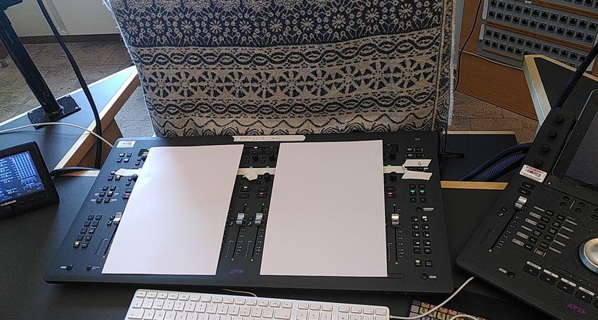
Alice Backlund
2022
download website (Cambridge Music Technology, 2022). The first mix aimed to have a
rhythmically and tonally “full” sound, utilizing 28 of the 51 available tracks. Another aim of
the mix was also to be “unassuming”, without distracting or harsh instruments so the focus of
the listeners’ attention would be on the panning tracks and not the song itself. This led to
tracks such as harmonica or tambourine being omitted from the “full” mix (for track list, see
Table 5 in appendix). The second mix aimed to only use the bare minimum of tracks to
convey a cohesive song whilst also masking the instrument audio object stimuli as little as
possible. This resulted in only using the bass drum, bass guitar, and acoustic guitar for the
sparse mix.

The instruments used for panning (as audio objects) were the lead vocal track and a
glockenspiel track. These were chosen partly because they represent different spectral
characteristics, as the lead (male) vocal had a broad spectral range and the glockenspiel had a
narrower spectral range, with its frequency content most prevalent from 1 kHz and upwards,
and also because each of their melodies were easy to follow. The decision to use these tracks
was inspired by Lee and Rumsey’s (2013) work which utilized male speech in their
experiment, as well as Pulkki and Karjalainen’s (2001) findings that audio objects with a
spectral range over 1.1 kHz are localized differently than audio objects with a wider
frequency spectrum.

The original instrument files were brought into Pro Tools and each different combination of
panning amount and panning side was recorded to individual stereo files. This was to have the
panning amount “printed” onto the tracks and avoid possible errors later in the process. The
files were exported and named according to a key from a file name system. This not only
helped with creating randomization for each Pro Tools session but also with secrecy as no file
name contained any information about what kind of panning the track had.

Table 2 – Specification of the instrument files

 Instrument Angle Pan Side
 (PT Panning amount)
 Vox 05° (17) L
 Vox 05° (17) R
 Vox 15° (50) L
 Vox 15° (50) R
 Vox 25° (83) L
 Vox 25° (83) R
 Glockenspiel 05° (17) L
 Glockenspiel 05° (17) R
 Glockenspiel 15° (50) L
 Glockenspiel 15° (50) R
 Glockenspiel 25° (83) L
 Glockenspiel 25° (83) R

2.3 Equipment
The equipment used for the experiment was an Avid Pro Tools S3 control surface, and
Genelec 1030 A loudspeakers in a stereo setup with a 60° base angle according to ITU-R
BS.2159-6.

 10

Alice Backlund
2022
2.4 Participants
20 participants took part in the listening test. One of the participants was omitted due to a
misunderstanding in the execution of the test, making the results of this participant unusable.
Therefore, the total amount of legitimate participants was 19. All participants were current
students of the sound engineering program at the Luleå University of Technology.

2.5 Procedure
2.5.1 Task Procedure
The task was to match the perceived placement of an audio object, that was placed on one
track, to another audio object on a reference track by the use of panning. The participants
were informed that they were going to focus on one pair of tracks at a time, matching the
perceived position of the reference audio object on the first track to the other. They could use
the solo button to toggle between the different tracks, as they were in solo latch mode, see
“Pro Tools Sessions” below. When they felt that the perceived position was the same on both
tracks, they were to click on the “nudge” button twice to continue to the next pair. The
participants were allowed to set their own listening loudness level as well as starting or
pausing the music at their own will (as the material was on a loop).

Participants were also informed that there would be two sets, with twelve tracks each. The
difference between each set was the background mix, being either full or sparse (in a
randomized order). Each pair of tracks in Pro Tools were assigned different colors. The colors
were shown on the control surface above the channel strip display and were also brought to
the participants’ attention as a tool for keeping track of the pairs of tracks as well as alerting
them when they were finished with each set. To alert the participants of when they were
finished with each set, there were empty tracks in between the sets which were colored
yellow, and so the participants were instructed to alert the supervisor when they had reached
the yellow tracks in order for the next set to begin.

2.5.2 S3 Control Surface
To simplify the task, only two channels were available for the participants. Regular paper was
used to cover the other tracks. Masking tape was placed over the channel strip display so
participants would not know what panning amount they had chosen. The computer screen was
also covered with fabric so no information on chosen panning amount could be detected.
Masking tape was also placed on the panning knob of the track with the fixed panning
amount, as to make it clear which panning knob of which track the participants was supposed
to move. The nudge button was marked with an arrow.

 11

Alice Backlund
2022

Figure 3 - S3 Control Surface Setup

2.5.3 Pro Tools sessions
There were individual Pro Tools sessions created for each participant, with randomized order
of the stimuli tracks as well as the mixes. The mixes were in “solo safe” mode, meaning that
the solo function of other tracks would not affect them. Starting the session, only one mix was
soloed and the other one was muted. The Pro Tools session itself was in a solo latch option
called “X-OR” meaning that soloing a track cancels the previous solo. This practically meant
that the participants could listen to one mix at a time as well as simultaneously toggle between
the different tracks.

Before starting their second set of the listening test, the subjects were asked to step away from
the desk, so the supervisor could mute the previous mix track and unmute the next mix track.
The fabric covering the computer screen had to be uncovered to do this. Therefore, in case
any subject was to take this as an opportunity to glance at the computer, it became important
to maintain an amount of secrecy in the Pro Tools projects. Consequently, all tracks were
named after a key. Only the mono tracks that were going to be panned were named after their
respective instrument and thus did not give away any crucial information.

2.6 Testing of Data
The data gathered from the listening tests were looking at the panning deviation for each
participant’s answers (see “3.1 Panning Deviation”). The distribution of the answers were
divided into histograms according to the factors of the listening test. When comparing the
data, analysis of variance was the method of choice, looking at the main effects of the
different factors. Interactions between the different factors were therefore not examined. An
F-test and t-test with the significance value of 0.05 were conducted within the different levels
of the factors. Mean value and standard deviation was also calculated.

 12

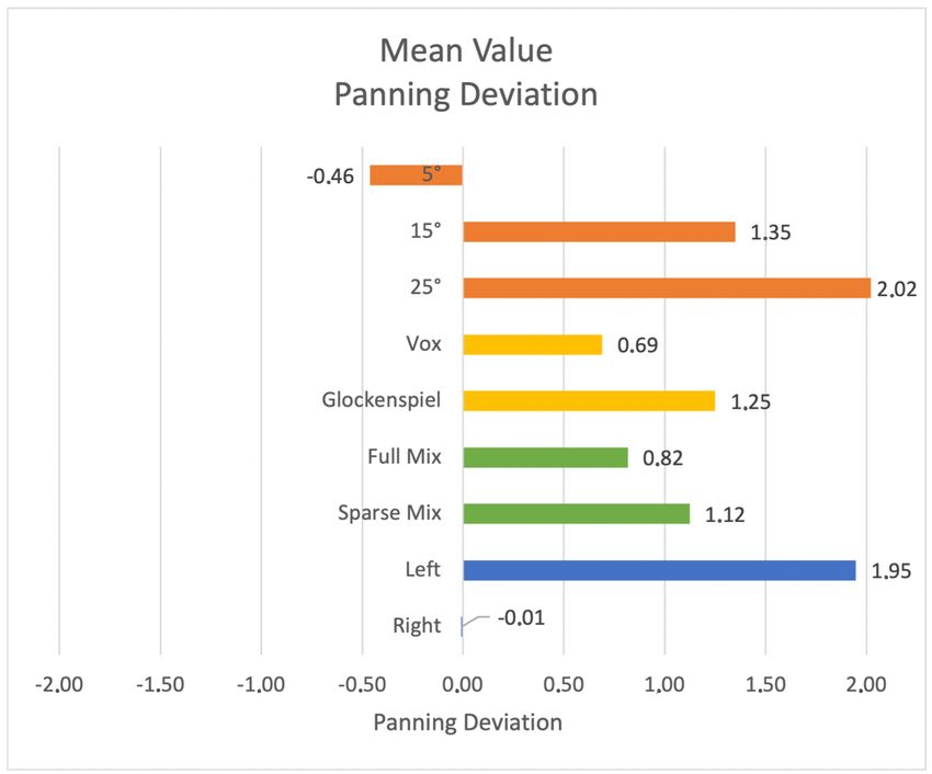
Alice Backlund
2022

 3. Results & Analysis
3.1 Panning Deviation
The term “panning deviation” refers to how close a subject’s placement of a panning track
was to a specific panning amount. In Pro Tools, the panning amount goes from 0 to 100 on
both sides, with 0 being center panning and 100 being full panning. To illustrate how this
coincides with “panning deviation”, the 15° angle corresponded with Pro Tools panning
amount 50 out of 100. If a subject placed the panning track at panning amount of 50, this
would be the correct amount and noted down as 0 in panning deviation. Say that the subject
had placed it at 58, then 58 would be 8 amounts too wide, noted down as +8 in panning
deviation. If the subject had placed the track at panning amount 42, then that panning amount
would be considered 8 amounts too narrow, noted down as -8 in panning deviation. All
graphs below will be presented according to panning deviation.

3.2 Mean Value and Standard Deviation
The mean value of panning deviation was calculated for each factor. The results range from
-0.46 to +2.02 since they take negative values of panning deviation into account.

Figure 4 - Mean value of panning deviation

 13

Alice Backlund
2022
Table 3 demonstrates the standard deviation values applied to each category of factors from
the listening experiment. Since standard deviation measures the spread around the mean
value, high values in standard deviation imply a higher amount of panning deviation for the
category.

Table 3 - Standard deviation results applied to panning deviation for each category

 Category Standard Deviation
 5° 07.39
 15° 08.97
 25° 11.54
 Vox 08.05
 Glockenspiel 10.76
 Full Mix 09.38
 Sparse Mix 09.62
 Left 09.38
 Right 09.52

3.3 Category Results
The star symbol refers to outliers in each category. Each figure has a graphic distinction of the
panning deviation amount -1 to +1 as an aid of distinguishing what is considered to be the
column that represents a correct assessment in panning, e.g. on target.

Figure 5 - Panning deviation of 5° audio objects

 14

Alice Backlund
2022

Figure 6 - Panning deviation of 15° audio objects

Figure 7 - Panning deviation of 25° audio objects

 15

Alice Backlund
2022

Figure 8 - Panning deviation of the audio object category “Instrument”

Figure 9 - Panning deviation of the audio object category “Mix”

 16

Alice Backlund
2022

Figure 10 - Panning deviation of the audio object category “Panning Side"

3.4 t-test and F-test
Table 4 shows the p-values from two-tailed paired sample t-tests, as well as the p-values from
F-tests. The tests were applied to panning deviation values for each category and both tests
have a significance level of 0.05. Significant results are distinguished by yellow cells. The t-
test for the category 5° to 15° could be considered close to a significant result.

Table 4 – P-values from t-test and F-test

 Test category t-test F-test
 5° to 15° 0.069 0.018
 5° to 25° 0.024 0.00000007
 15° to 25° 0.550 0.002
 Instrument 0.430 0.00001
 Mix 0.670 0.709
 Sides (left/right) 0.013 0.824

 17

Alice Backlund
2022

 4. Discussion
4.1 Angles
A clear observation when comparing the different results for the different angles is that 5° and
15° have a normal distribution, whereas 25° does not. Why 25° does not have a normal
distribution in its panning deviation result is mostly due to an overrepresentation in the
panning deviation category from +17 to +19. The high frequency of answers in that category
for 25° can be explained simply that those occur when subjects have placed the reference
track to the widest amount possible. 25° equals 83 in Pro Tools amount, and 30° is 100 in Pro
Tools panning amount, making the difference in panning amount 17.

Additionally, the panning deviation amount +17 has the frequency of 24 for 25°, whereas
being only once represented outside of 25°, with one subject having the panning deviation of
+17 at 5°. The panning deviation amounts +18 and +19 had no representation. This means
that in the diagrams for the other categories, within the panning deviation amount +17 to +19,
almost all of them are 25° objects that have been placed at the widest possible angle.

When designing the listening experiment, the panning angle of 25° was chosen because it
would enable subjects to place their audio objects under as well as over 25°. The reasoning
behind choosing the 25° panning angle was because Pro Tools panning functions do not allow
further panning than 100/30°, as it stops at that amount. Because the panning stops at that
amount, there would not have been a way of knowing if subjects perceived objects placed at
the 30° angle at a wider angle. Also to note, if there would have been a way to place objects at
a further angle than the maximum amount of 30°, when regarding the results for the 25°
angle, there would have been a plausibility that the results could have been even more spread
out and would not have a high frequency at the panning deviation value +17.

Additionally, the manual panning tool on the S3 Control Surface was a continuous panning
knob and did not physically stop at any panning amount. In practice, this resulted in that even
though the panning amount had reached its maximum, the panning knob did not physically
cue this boundary by stopping its rotation. Therefore, if the 30° angle had been chosen, there
would also have been a risk that subjects could have accidentally and not consciously placed
the object at the 30° position. This is because they would not have known that they had
reached that point because they were not given any visual cues of their panning decisions. For
this reason, if 30° had been the chosen angle, the results could have created a threshold effect
that could have been misinterpreted as a high amount of panning accuracy, adding to the
motivation of choosing the angle of 25° for the experiment.

When comparing the results for 5° and 15°, 15° had a considerable amount of outliers (5) and
skewing slightly to the positive side, as there were 74 answers over the panning deviation
amount +1 and 53 answers under the panning deviation amount -1. This means that the
subjects had a slight tendency to place the 15° objects wider than the correct position. 5° had
the narrowest spread of 34, whereas 15° had a spread of 67 and 25° had a spread of 42.
Additionally, 5° had the highest frequency in category -1 to +1 in panning deviation out of all
angles, with a frequency of 34 compared to the frequency of 25 for 15° and 17 for 25°. The F-
test also showed a significance in the difference between the angles 5° and 15° (p = 0.018).

Not only were there a significance in the difference between the angles 5° and 15°, but the
standard deviation values also point to a lesser degree of panning accuracy for the wider
angles. The standard deviation applied to the panning deviation values for 5° was the smallest
with 7.39, whereas 15° had an 8.97 standard deviation and 25° had a standard deviation value

 18

Alice Backlund
2022
of 11.54. These results are in line with the argument that Lee and Rumsey (2013) and Blauert
(1997) make about localization blur, that wider angles suffer from greater localization error
due to an increase in interaural differences.

There are additional results for the F-tests and t-tests that show significance in the additional
different combination of angles, these results are from tests compared with the 25° results.
However, since one of the terms of using t-tests and F-tests is normal distribution and the 25°
result does not have a normal distribution, these results cannot be applied.

4.2 Instrument
The results for the vocal track (“vox”) had more of a normal distribution than the glockenspiel
track. The F-test presented a significant difference between the results (p = 0.00001). When
looking at the mean value of panning deviation, the vocal track also had a slightly lower result
than the glockenspiel. Furthermore, the vocal track had a considerably higher frequency in the
panning deviation category -1 to +1 than the glockenspiel track, with a frequency of 44
compared to 32. This could be an indication that subjects could generally come closer to the
correct panning amount when panning the vocal track than when panning the glockenspiel
track.

Another argument for this indication is that the previously mentioned error of placing 25°-
objects at 30° is overrepresented for the glockenspiel track. This could be explained by
considering that the glockenspiel track had a narrow spectral range, as well as having its
frequency content most prevalent from 1 kHz and upwards, and that Pulkki et al. (2011) states
that localization is dependent on the spectrum of the signal, making a signal with a narrow
bandwidth more difficult to locate.

4.3 Mix
One of the major points of creating the listening test was to see if different types of mixes
would have any effect on the participant’s localization ability. The results show that there is
no significant difference in panning deviation in the mix category. The distribution of panning
deviation is more or less equal; additionally, the standard deviation values are very close for
the full and sparse mix, with 9.38 for the full mix and 9.62 for the sparse mix. There was no
significance from either the F- or t-test. Therefore, out of the different factors for the
experiment, mix did not have a significant impact on the subjects’ performance.

4.4 Panning Side
Panning side refers to how the results of audio objects panned to the left or right differ from
each other. Since panning deviation measures the accuracy from a specific point, this means
that the negative panning deviation is towards the center of the stereo sound field and the
positive panning deviation is towards the sides (see “3.1 Panning Deviation” for further
description). The distribution of panning deviation for the left-side-panning is skewed to the
positive side, with 119 answers above the panning deviation amount +1 and 68 answers below
-1. The right-side-panning distribution is somewhat skewed to the negative side, with 90
answers above +1 and 103 answers below -1.

There can be a tendency of shifting the stereo image to the left based on the above-mentioned
results. Because the left-side panning deviation is skewing positive, the tendency of panning
deviation is towards the left, as positive panning deviation is towards the sides. Moreover,
because the right-side panning deviation is skewing negative, and therefore being more
towards the center, the panning deviation is also leaning towards the left. Consequently, these
results show that the panning deviation is slightly shifted towards the left. The mean value of
 19

Alice Backlund
2022
panning deviation as seen in Figure 4, where the left-side mean value is +1.95 and the right-
side mean value is -0.01, shows that there is some difference in the perception of audio
objects panned to the left.

Since the t-test shows significance in this category (p = 0.013), this means that this result is
most likely not a coincidence. This could be due to the fact that the listening room is
asymmetrical, being smaller toward the left of the listening position and larger towards the
right. Even though the room is acoustically treated, the shape of the room could have affected
the results.

4.5 Critique of Method
There are some points to mention when it comes to conducting the listening tests. Firstly,
when describing the test, it was not mentioned what the panning tracks actually consisted of.
This led to some confusion amongst a few subjects, as they had to find out on their own that
the different tracks were glockenspiel and male vocals.

Secondly, one participant misunderstood the instructions and panned the objects to match
their “mirror image”; e.g., if they heard the reference track from the left, they would pan the
other track to the right side. Consequentially, the participant’s answers were omitted from the
results. This was a mistake in the delivery of the instructions, and thus all later participants
were alerted to specifically not only to match the placement but also the side of the reference
track.

One difficulty with the method was specifically with solo functions in Pro Tools. If a subject
clicked twice on the same solo button, the track would be un-soloed and all tracks in the
project would play at the same time. This caused a sudden and uncomfortable increase in
loudness, more or less scaring the subject. At the time of conducting the tests, a solution to
this problem could not be found. Comparatively, in the DAW Logic, if a track is muted and
soloed at the same time, the solo function overrides the mute function. The mute function
overrides the solo function in Pro Tools, causing this problem. Therefore, all participants were
alerted in the instructions that this was something that could happen. Only one out of twenty
participants managed to not accidentally un-solo a track.

Moreover, another small but notable issue with the method had to do with the color-
coordination of the tracks. All pairs of tracks were in different colors as a system of keeping
track of the pairs, as well as alerting the subjects when they had completed the first set. These
colors could be seen on the control surface. The participants were asked to look out for the
color yellow, as this meant “stop” (because these were the empty tracks between each set).
Many participants were confused as to which shade of yellow this would be, mistaking orange
for yellow, or simply forgetting what color to look after. This became a point of distraction. A
possible solution could have been to choose the color red for the empty tracks, as red is often
associated with “stop”. Another solution could have been to place a sign on the control
surface saying “yellow = stop”, as this might have relieved the subjects with retaining the
information about the color and given them more mental energy to focus on the task at hand.

4.6 Findings and Future Applications
The purpose of this study was to take a closer look at the gap within the area of research,
specifically to look at the effect of localizing sounds within a musical mix. When comparing
the results from the different mixes, both mixes gave similar results. Therefore, the
differences between the mixes had no impact on localization accuracy. However, instrument
and panning angle showed significance in the results, namely that the glockenspiel with a

 20

Alice Backlund
2022
narrower bandwidth was more difficult to accurately locate, as well as audio objects placed at
25°. This aligns with the results of previous studies such as Pulkki and Karjalainen (2001) as
well as Lee and Rumsey (2013) who showed that localization is dependent on frequency
content and panning angle.

Regarding future research, further studies could take a closer look at what different variables
might affect localization accuracy. Even though the study did not find any significance
between the sparse and full mix, the usage of musical sources in these studies remains an
interesting topic as it lies closer to the ecological sounds that are utilized when mixing audio.
Since the listening room might have affected the results, future studies could explore what
effect headphone monitoring could have on the results if the method of this listening
experiment were to be applied.

 21

Alice Backlund
2022

 5. References
Blauert, J. (1997). Spatial Hearing (rev. ed.). MIT Press.

Cambridge Music Technology. (2022). The ‘Mixing Secrets’ Free Multitrack Download
Library. https://cambridge-mt.com/ms/mtk/#BenCarrigan

Izhaki, R. (2012). Mixing Audio: Concepts, Practices and Tools (2nd ed.). Focal Press.

Lee, H., & Rumsey, F. (2013). Level and Time Panning of Phantom Images for Musical
Sources. J. Audio Eng. Soc., 61(12), pp. 978-988.

Lee, H. (2017, May 20-23). Perceptually Motivated Amplitude Panning (PMAP) for Accurate
Phantom Image Localisation [Conference paper]. AES 142nd Convention, Berlin, Germany.
http://www.aes.org.proxy.lib.ltu.se/e-lib/browse.cfm?elib=18646

Pulkki, V. & Karjalainen, M. (2001). Localization of Amplitude-Panned Virtual Sources I:
Stereophonic Panning. J. Audio Eng. Soc., 49(9), pp. 739-752.

Pulkki, V., Lokki, T., & Rocchesso, D. (2011). Spatial Effects. In U. Zölzer. (Ed.), DAFX:
Digital Audio Effects (pp. 139–183). Chapter, J. Wiley and Sons.

 22

Alice Backlund
2022

 6. Appendix A
Table 5 – Track lists for each mix created for the experiment

 Tracks used for “Full Mix” Tracks used for “Sparse mix”
 02 Kick 02 Kick
 03 Kick Sample 03 Kick Sample
 04 Snare
 05 Snare Sample 1
 06 Snare Sample 2
 08 Tom 1
 09 Tom 2
 11 Cymbal Sample 1
 12 Cymbal Sample 2
 17 Hand Claps
 18 Bass 18 Bass
 19 Acoustic Gtr 1 19 Acoustic Gtr 1
 22 Piano
 23 Organ
 26 Glockenspiel* 26 Glockenspiel*
 27 Violin 1
 28 Violin 2
 29 Viola
 30 Cello
 31 Strings Mix
 33 Violin Samples
 34 Viola Samples
 35 Cello Samples
 40 Lead Vox* 40 Lead Vox*
 42 Backing Vox 2
 43 Backing Vox 3
 44 Backing Vox 4
 45 Backing Vox 5
 * Used as instrument audio Sparse mix had an additional EQ
 objects on the mix bus; low shelf at 100 Hz,
 -3 dB.
Names according to track list folder from source (Cambridge Music Technology, 2022).

 23