Load Forecasting in District Heating Networks: Model Comparison on a Real-World Case Study
←
→
Page content transcription
If your browser does not render page correctly, please read the page content below
Load Forecasting in District Heating Networks:
Model Comparison on a Real-World Case Study

    Federico Bianchi, Alberto Castellini, Pietro Tarocco, Alessandro Farinelli

                Verona University, Department of Computer Science,
                     Strada Le Grazie 15, 37134 Verona, Italy,
                    {federico.bianchi,alberto.castellini,
                pietro.tarocco,alessandro.farinelli}@univr.it

                             Accepted version.
            The final authenticated version is available online at
              https://doi.org/10.1007/978-3-030-37599-7 46

       Abstract. District Heating (DH) networks are promising technologies
       for heat distribution in residential and commercial buildings since they
       enable high efficiency and low emissions. Within the recently proposed
       paradigm of smart grids, DH networks have acquired intelligent tools able
       to enhance their efficiency. Among these tools, there are demand fore-
       casting technologies that enable improved planning of heat production
       and power station maintenance. In this work we propose a comparative
       study for heat demand forecasting methods on a real case study based on
       a dataset provided by an Italian utility company. We trained and tested
       three kind of models, namely non-autoregressive, autoregressive and hy-
       brid models, on the available dataset of heat demand and meteorological
       variables. The best model, in terms of root mean square error of predic-
       tion, was selected. It considers the day of the week, the hour of the day,
       some meteorological variables, past heat loads and social components,
       such as holidays. Results show that the selected model is able to achieve
       accurate 48-hours predictions of the heat demand in several conditions
       (e.g., different days of the week, different times, holidays and workdays).
       Moreover, an analysis of the parameters of the selected models enabled
       to identify a few informative variables.

Keywords - Heat load forecasting, district heating network, linear regression
models, model interpretability, time series analysis.

1    Introduction
The heating and cooling demand in the residential sector in Europe is responsible
for a share of about 40% of the overall final energy usage [16]. District Heating
(DH) networks are acknowledged as a promising technology for heat distribu-
tion, covering the demand of buildings, providing higher efficiency and better
pollution control. A DH network is a network in which the heat is generated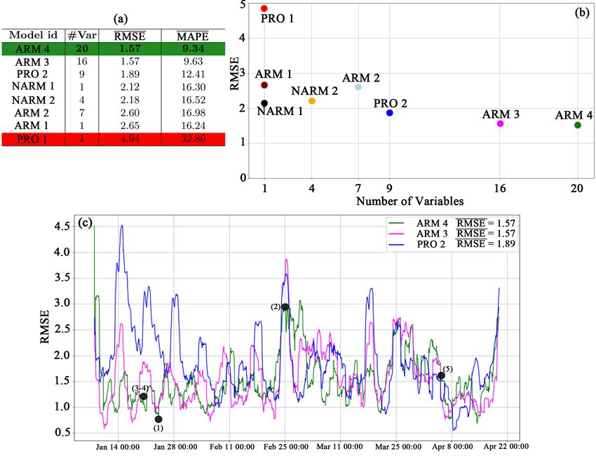
in one or more centralized locations and distributed through a pipe system via
exchangers in buildings (see Figure 1). The management of the system is based
on seasonal heating temperature. The combination of flow and temperature (i.e.
power) must be high enough to cover the demand of the entire network and also
the heat losses [5]. Key analytical tools for optimizing the heat production for
DH networks are load forecasting models. They consists of a set of statistical
and artificial intelligence methods for predicting the future heat demand, given
the past evolution of the demand and some environmental factors that influence
it. Accurate models for heat load forecasting have significant advantages such
as improved energy efficiency of heat production and reduced environmental im-
pact. This topic has recently gained strong interest from the artificial intelligence
research community in the context of smart grids, namely, energy networks using
intelligent agents to optimize their functioning.
    Several predictive models have been designed for short-term load forecasting
(STLF) and the literature contains a variety of applications and models. The
application domain which mostly resembles our domain of interest is electricity
demand forecasting, for which an extended literature is available [8,9]. Models
that can be classified into two main categories, namely, statistical approaches
for time series forecasting, mainly based on autoregressive integrated moving av-
erage (ARIMA) models, and machine learning/artificial intelligence techniques,
such as gaussian processes, artificial neural networks, fuzzy logic and support
vector machines. Statistical time series models, pioneered by Box-Jenkins [1] and
Holt Winters [7] methods, are the earliest forecasting methods. ARIMA mod-
els [8] are usually applied in univariate scenarios for short horizons. A number
of studies apply seasonal ARIMA (SARIMA) techniques to STLF [17,12,3,11]
to model seasonal patterns, and ARIMAX in multivariate scenario to simulate
the effects of weather and the day of the week on the future demand. Multiple
linear regression is proposed in [15,5,4] to consider multiple relationships be-
tween weather conditions, social components (such as holidays and weekdays)
and future demand. Comprehensive reviews of the literature are provided in
[6,13,14,8].
    DH heat demand forecasting models normally consider two factors: weather
conditions and the social components. The weather is the most significant factor
affecting the consumption, however, according to [19] most of the past publi-
cations made use of temperature as the main variable and only a few of them
consider other components as relative humidity, wind and rainfall. The social
component of the consumption describes the behaviour of customers and can be
interpreted in terms of annual, weekly and daily patterns. There exist two main
approaches namely using a single-equation model for all the hours or multiple-
equation models with specific equations for each hour of the day. The latter
approach has been adopted for instance in [15,17]. Other relevant social compo-
nents are calendar events [2], such as holidays which have different behaviours
than working days, leading to systematic variations in the heating load. A pos-
sible approach consists in building different models for normal and special days
of the week [15], if enough data are available.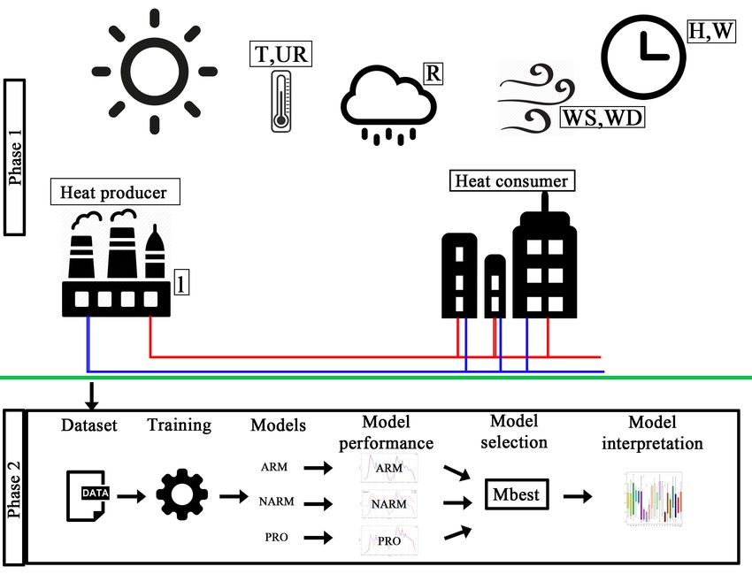
In this work we present a comparative study of heat demand forecasting
methods on a real case study based on a DH network managed by an Italian
utility company, AGSM1 . The heating network is located in Verona, Italy. The
dataset concerns the hourly heating load produced by 3 sites in 2016, 2017 and
2018. Data from 2016-17 have been used to train the models and data from
2018 to test them. The comparison is made among three modeling frameworks,
namely, non-autoregressive models, autoregressive models and hybrid method
called Prophet [18]. Different parameter configurations have been tested, obtain-
ing a total of 8 models to compare. Results show that one of the autoregressive
models reached the best performance in our specific case study. An analysis is
made to interpret the models and discover common behaviors in different week-
days and hours of the day. The main contributions of this work to the state of
the art are summarized in the following points:

    · we compared the performance of 8 models on a real case study of heat
      demand forecasting and we identified the best model for our context.
    · we analyzed the performance of the best model in different time instants,
      such as, working days, weekends, holidays.
    · we analyzed the parameters of the best model and provide a first interpre-
      tation of the most significant variables for 48-hours forecasting.

    The rest of the manuscript is organized as follows. Section 2 presents the
framework for model comparison, the dataset, the used methodologies and the
performance measures. Result and performance are analyzed in Section 3. Con-
clusions and future directions are described in Section 4.

2     Material and Methods

In this section we formalize the problem, describe our dataset of heating loads
and meteorological parameters, introduce the modeling methodologies and define
the performance measures used to compare different models.

2.1    System overview and problem definition

The district heating, illustrated on top of Figure 1 is a centralized network where
the heat is produced and distribuited through a pipe system to commercial and
residential buildings with subsequent return to the power station. The utility
company controls the demand variability with flow in according to seasonal
operation temperature. The supplied temperature and flow must be high enough
to cover the customers’ demand and provide better control of pollution, using
renewable energy. The aim of the present work is identify models which allow
us to optimize the heat load forecasting in the next 48 hours and find out which
variables are significant on forecasting the heat demand.
1
    https://www.agsm.it/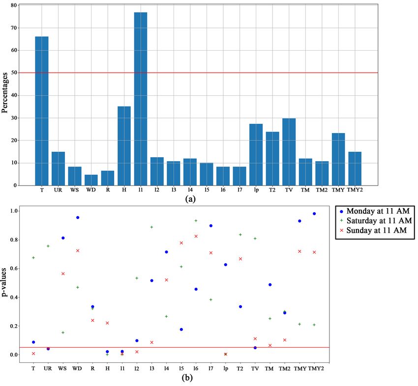
The bottom of Figure 1 is an overview of the process we used to select
the best model for heat demand forecasting. The dataset provided by utility
company is used to train different statistical models. Here we consider three
kinds of methods, namely, non-autoregressive, autoregressive and hybrid models
generated Prophet. After the generation of models we evaluate the performance
and select the model that better fits the data. The models are evaluated with
standard performance measures. Finally we use the selected model to forecast the
heat demand and analyze the parameters in order to identify the most significant
variables.

Fig. 1. Framework for model comparison: Phase 1 → (a) District heating network
(data acquisition). Phase 2 → (b) Heat forecasting: model selection

2.2   Dataset
In this work we used real world data provided by AGSM, related to years 2016,
2017 and 2018. The sampling interval is of an hour, with 12792 of total ob-
servations. Considering the switching on/off of DH is controlled at level of the
public administration, data concerns only the coldest parts of the year, in fact
our work focuses on predicting the heating load consumption only when the
heating is on. We used data from 2016-2017 (01 January 2016 - 11 May 2016,
11 October 2016 - 14 May 2017, and 16 October 2017 - 31 December 2017,
10296 observations in total) to train the models. Data from 2018 (08.01.2018 -
21.04.2018, 2496 observations) were used for testing. Variables available in raw
datasets were temperature, relative humidity, wind speed, wind direction, rain-
fall and load consumption of the DH system. We generated two kinds of new
variables, based on weather and load components. The complete list of variables
is reported in Table 1.

Symbol   Description                           Symbol
                                                   Description
l        Heating load [MW]                     T   Temperature [°C]
l1       Heating load of the previous day      UR  Relative humidity [%]
l2       Heating load of 2 days before         WS  Speed of wind (m/s)
l3       Heating load of 3 days before         WD  Direction of wind. Cardinal
                                                   directions encoded from 0 to
                                                   9 (9 = no wind)
l4       Heating load of 4 days before        R    Rainfall. 1 = rain, 0 = oth-
                                                   erwise
l5       Heating load of 5 days before        TV   Moving average of tempera-
                                                   ture on seven previous days
l6       Heating load of 6 days before        TM   Maximum temperature of
                                                   the day
l7       Heating load of 7 days before        TS   Square temperature
lp       Peak load of previous day at 6:00 AM T2   Square of maximum temper-
                                                   ature
H        Holiday (0 = false, 1 = true)        TMY Maximum temperature of
                                                   the previous day
W        Weekend (0 = false, 1 = true)        TMY2 Square of maximum temper-
                                                   ature of the previous day

                             Table 1. List of variables

2.3   Models

We proposed three kinds of model, namely: Non-Autoregressive Model (NARM),
Autoregressive Model (ARM) and Prophet (PRO) described below and summa-
rized in Table 2.
    Non-Autoregressive Model (NARM). It is built through a process known
as binary recursive partitioning, which is an iterative process that splits the data
into partitions (or branches) having similar properties (e.g., weekday, hour), and
then continues splitting each partition into smaller groups as the method moves
down each branch. The various branches refer to hour of the day, day of the week,
heating on/off. The aim of this method is to analyze the fundamental compo-
nents of the data in order to investigate if there are any (linear) relationships
between the heat demand and some independent variables in specific days of the
week and hours of the day. The models are generated after splitting the data into
partitions and this kind of approach is useful because, for example, if we have to
make predictions on Monday at 8:00 AM, we just need to access the model that
was trained with data in the same day and time in the past. We generated two
types of linear regression models, called NARM 1 and NARM 2 in the following,
that use a tree structure and no autoregressive variables, such as delayed load.
NARM 1 is a set of day/hour univariate linear regression models (168 models
in total) where every model is related to a specific pair (weekday,hour) and has
the form l = C1 T + C0 , where C0 , C1 are coefficients and T is the temperature.
NARM 2 differs from NARM 1 in the independent variable, since it uses, in
addition to T , variables U R, W S and W D. The learning methodology used is
ordinary least squares that fits a linear model with a vector of coefficients that
minimize the residual sum of squares between the observed responses in the data
and the responses predicted by the linear approximation.
Autoregressive Model (ARM). It is a statistical method to characterize
the impact of one or more independent variables on a dependent variable, in
order to evaluate the linear dependency between them. Here we propose four
types of linear regression models, in which the heat consumption l is explained
by a liner model based on weather variables: T, UR, WS, WD and R. Besides
the weather factors, we include social components factors like annual, weekly,
daily patterns of consumption and calendar events, distinguish workdays from
weekend. The proposed models are called ARM 1, ARM 2, ARM 3 and ARM
4 in the following. All of them are autoregressive because they consider delayed
load. In ARM 1 and ARM 2 we adopted a single-equation model strategy. The
latter uses 7 delayed loads, from one day before the forecasting instant to 7 days
in advance. In ARM 3 we used a multiple equations strategy with one model for
each hour of the day (i.e., 24 models in total), while in ARM 4 we used a multiple
equations strategy with one model for each pair (weekday, hour) (i.e., 168 models
in total). In ARM 4 we forecast the load for each day and for each hour of the
day with different equations, therefore we have 168 forecasting equations having
the following form:
Mij = f (W, dl, social) (1)
where i ∈ {1, . . . , 7} refers to day of week, j ∈ {0, . . . , 23} refers to hour of the
day, W refers to weather variables and derived variables. The autoregressive part
of the method is represented by dl and it refers to past loads. These variables
measure the load a day before the prediction (at the same hour), 2 days before
the prediction and so on, until 7 days before the prediction. We also considered
the peak of energy demand at the previous day, which is at 6:00 AM in our case.
Social refers calendar events, such as working days or holiday. These dummy
variables are important because they model the different demand during differ-
ent days of the week, in fact during the weekend and holiday we can observe
that the heat demand is lower. In ARM 3 and ARM 4 we followed the [15] idea,
considering a multiple equations approach. Here we include more than one me-
teorological factors such as, T, UR and R. We do not consider lagged errors but
7 lagged loads to enforce the forecast accuracy.
Prophet (PRO). It is an open source library published by Facebook2 [18]
that provides the ability to make time series prediction, but it is also designed to
have intuitive parameters that can be adjusted without knowing the details of the
2
https://research.fb.com/prophet-forecasting-at-scaleunderlying model. At its core, the Prophet procedure is similar to a generalized
additive regression model (GAM) [10] with four main components: a piecewise
linear or logistic growth curve trend g(t), a yearly seasonal component modeled
using Fourier series s(t), a weekly seasonal component using dummy variables
h(t) and the error term εt :
y(t) = g(t) + s(t) + h(t) + εt . (2)
The GAM formulation has the advantage to be flexible, accommodating sea-
sonality with multiple periods, it fits very fast and parameters are easily inter-
pretable. Here we use two types of Prophet model: PRO 1 and PRO 2. PRO 1
considers only the historical load component to predict the next 48 hours. PRO
2 also uses regressive components of load, starting from prediction instant and
considering loads from a day to seven days in the past.
Model id
Description
ARM 1 It is an Autoregressive Model and only l1 is considered
ARM 2 It is an Autoregressive Model and we considered l1, l2, l3, l4, l5, l6, l7
ARM 3 It is an Autoregressive Model and we used li delayed loads (i ∈ [1, 7])
with weather variables such as T, UR, WS, WD, TV, TM and social
components as H, W, lp
ARM 4 It is an Autoregressive Model equal to ARM 3 but we also used R, TS,
TM2, TMY and TMY2
NARM 1 It is a Non-Autoregressive Model and we used only T
NARM 2 It is a Non-Autoregressive Model and T, UR, WS, WD are considered
PRO 1 Prophet Model and we considered only l
PRO 2 Prophet Model and we also considered T, UR, l1, l2, l3, l4, l5, l6, l7
Table 2. Models description
2.4 Performance measures
Models were evaluated by two standard performance measures for time-series
forecasting, namely, the Root Mean Square Error (RMSE) and the Mean Abso-
lute Percentage Error (MAPE). Given an observed time-series with n observa-
tions y1 , . . . , yn and a prediction ŷ1 , . . . , ŷn , the RMSE is computed as formula:
v
u
u1 X N
RM SE = t (ŷt − yt )2 (3)
N t=1
and it represents the average error that the prediction makes each time in-
stant. The MAPE is computed as formula:N
1 X |ŷt − yt |
M AP E = ( ( )) · 100% (4)
N t=1 yt
and it represents the absolute average percentage error that the prediction
make it. Since we are interested in evaluating our models on 48 hours forecast-
ing in 2018, we computed these measures on heating load of 48 hours sliding
windows, starting from each time instants available in our dataset of 2018. Then
we averaged these numbers obtaining what we call average RMSE (RM SE) and
average MAPE (M AP E) in the following.
3 Results
Here we present a comparative evaluation of the models described in the previous
section. In the first part of the analysis (see Figure 2) we perform a comparison
of the global performance (i.e., RM SE) to select the best model. In the second
part (see Figure 3) we observe some 48-hour predictions of the best model in
specific time instants of 2018 (e.g., different days of the week, hours of the
day, holidays/workdays) and compare them to real heat demand in the same
moments to understand how the model behaves in different situations. Finally,
in the third part of the section (see Figure 4) we analyze the parameters of the
best model and identify some variables having stronger impact on the quality of
the prediction.
Best model selection. We compare the eight models summarized in Fig-
ure 2.a. The table shows the number of variables used in each model, the av-
erage root mean square error and the average mean absolute percentage error.
The models are ordered by RM SE. Model ARM 4 (highlighted in green) has
the best performance. The multiple-equation model, using one equation for each
pair of weekday and hour and 20 independent variables, proves to be accurate in
forecasting. ARM 3 assuming a multiple-equation model with one equation for
each hour of the day and 16 variables, performed equal to ARM 4 (RM SE), but
it achieved worse M AP E. PRO 2 follows closely whereas PRO 1, highlighted
in red, has the worse performance. The scatter plot in Figure 2.b, which repre-
sents the relationship between the number of variables used in a model and the
RMSE, shows that models with high numbers of variables have lower error. Fig-
ure 2.c shows the time evolution of the RMSE computed for 48-hour predictions
by the best 3 models. Each point (x,y) represents the RMSE (coordinate y) of
a 48-hours forecast starting at instant x. ARM 4 has a smaller error than ARM
3 and PRO 2. In Figure 2.c we also highlight 5 significant points that allow us
to focus on the model which obtained the best performance: ARM 4.
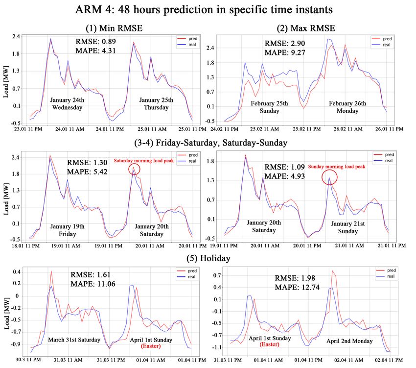
Comparison between real and predicted demand. In Figure 3 we show
the comparison between real and predicted demand in the 5 significant points de-
scribed in the following. Point (1) represents 48-hours forecasting with minimum
RMSE error which fits almost perfectly. Point (2) represents 48-hours forecasting
with maximum RMSE error. Notice that even though the error in that point isFig. 2. Comparison of model performance: (a) Table of number of variables, RM SE
and M AP E for each model. (b) Relationship between number of variables and RM SE
for the analyzed models. (c) RMSE of the best 3 models for each 48 hours forecast
performed in 2018. Each point (x,y) represents the RMSE (y) of a 48 hours forecast
starting at instant x
the highest, ARM 4 performs better than the other methods. Points (3-4) rep-
resent 48-hours forecasting in a weekend (i.e., Friday-Saturday and Saturday-
Sunday). The model is able to adapt to social components, forecasting quite
well working day as well as weekend, where the heat demand changes. It also
fits perfectly the load peak. Finally, (5) shows 48-hours forecasting on a holiday.
We show 48-hours forecasting starting from a day before Easter 2018 and from
Easter to Easter Monday. For each prediction, the method is able to fit load
peaks, adapting to load demand variations very quickly. The regression line is
less closest to the real load in (2) and in (5), even though the RMSE value is
still low.
Informative variables. In Figure 3 we show the parameters of the best
model. The bar plot (Figure 3.a) identifies the significant variables, in particular
it shows the percentage of models in which variables has p-values less than or
equal to 0.05. The scatter plot in Figure 3.b shows which variables are statisti-
cally significant for three specific models, namely, Monday, Saturday and Sunday
at 11. Figure 3.a show that 3 variables are very important: T, W and l1, in fact
they result significant for more than 65% of the models. Temperature T is par-
ticularly meaningful during evening and night when the temperature falls and
the heat demand increases in domestic buildings. The autoregressive variable l1
that refers to load demand of previous day is the most significant variable for
the method, having a p-values ≤ 0.05 for almost 80% of the models. The use ofFig. 3. ARM 4 - Best model: (1) 48 hours forecasting with minimum RMSE error. (2)
48 hours forecasting with maximum RMSE error. (3-4) 48 hours forecasting of weekend,
Friday-Saturday and Saturday-Sunday. (5) 48 hours forecasting of holiday: Easter
autoregressive variables as the load of the past days, in particular the previous
24 hours prior the forecasting instant, it seems to be crucial to predict the next
48 hours. An other autoregressive variable such as the load peak of the previous
day lp, it results meaningful for the model of 6 AM, when the first and the higher
load peak of the days occurs. This knowledge refines the forecasting capability of
the method. The other weather variables seem to have not considerable impact
for a good number of models.
In Figure 3.b we analyzed the significance of variables for three relevant
models such as Monday, Saturday and Sunday at 11 AM, when the second load
peak of the day occurs. From scatter plot we can see that lagged load l1 to
forecast the load at 11 AM is very significant for each selected models. The
model of Sunday considers the weather components as temperature and relative
humidity and also the autoregressive load variables. The variables l1 and lp
contain information concern Saturday morning at 11:00 AM and 6:00 AM, two
hours of the day when demand is higher. These variables allow Sunday to have a
precious knowledge about the load demand. The model of Saturday has almost
opposite behaviour than the other two models. It considers weather variables wederived: TM, TMY, T2, TMY2 and finally TV. The model of Monday considers significant only a few variables such as UR, H, l1 and TV. In particular we can notice that the variable lp is not important for the model, because refers to Sunday at 11 AM and it is a behaviour we expected. Fig. 4. Parameters of ARM 4 model: (a) the significant variables. (b) the significant variables for Monday, Saturday and Sunday models at 11 4 Conclusion and ongoing work We proposed a comparative study of models for demand forecasting in DH net- works. Models were generated and analyzed on a real-world dataset. We evalu- ated non-autoregressive, autoregressive and hybrid models performances in terms of RMSE and MAPE to find the best model. Model ARM 4 performed better than the others. It is an autoregressive model with multiple-equation approach with one equation for each pair (weekday, hour), with 168 equations in total. By analyzing the parameters of model ARM 4 we discovered that weather factors, delayed load and social components are crucial for accurate forecasting. This research can be widely extended in several directions. First, we will compare the presented models with models generated by other machine learning techniques, such as, Gaussian processes and neural networks. Then, we will investigate the
effects of solar radiation and other social components on heat load demand for
improving forecast accuracy. Finally, we will improve the analysis of model pa-
rameters to identify variables affecting the heat load in different days and hours.

Acknowledgments
The research has been partially supported by the projects ”Dipartimenti di
Eccellenza 2018-2022, funded by the Italian Ministry of Education, Universi-
ties and Research (MIUR), and ”GHOTEM/CORE-WOOD, POR-FESR 2014-
2020”, funded by Regione del Veneto.

References
 1. G. Box and G. Jenkins. Time series analysis: forecasting and control. Holden-Day,
    1976.
 2. M. Dahl, A. Brun, O.S. Kirsebom, and G.B. Andresen. Improving short-term heat
    load forecasts with calendar and holiday data. Energies, 2018.
 3. N. Elamin and M. Fukushige. Modeling and forecasting hourly electricity demand
    by sarimax with interactions. Discussion Papers in Economics and Business 17-28,
    Osaka University, Graduate School of Economics and Osaka School of International
    Public Policy (OSIPP), 2017.
 4. T. Fang. Modelling district heating and combined heat and power, 2016.
 5. T. Fang and R. Lahdelma. Evaluation of a multiple linear regression model and
    SARIMA model in forecasting heat demand for district heating system. Applied
    Energy, 179:544–552, 2016.
 6. E.A. Feinberg and D. Genethliou. Load Forecasting, pages 269–285. Springer US,
    Boston, MA, 2005.
 7. P. Goodwin. The Holt-Winters approach to exponential smoothing: 50 years old
    and going strong. Foresight: The International Journal of Applied Forecasting,
    pages 30–33, 2019.
 8. G. Gross and F.D. Galiana. Short-term load forecasting. Proceedings of the IEEE,
    75(12):1558–1573, 1987.
 9. M.T. Hagan and S.M. Behr. The time series approach to short term load forecast-
    ing. IEEE Transactions on Power Systems, pages 785–791, 1987.
10. T. Hastie and R. Tibshirani. Generalized additive models: Some applications.
    Journal of The American Statistical Association - J. AMER. STATIST. ASSN,
    pages 371–386, 1987.
11. R.J. Hyndman and G. Athanasopoulos. Forecasting: principles and practice. 2014.
12. M.S. Kim. Modeling special-day effects for forecasting intraday electricity demand.
    European Journal of Operational Research, 230:170–180, 2013.
13. P. Mirowski, S. Chen, T.K. Ho, and C.N Yu. Demand forecasting in smart grids.
    Bell Labs Technical Journal, pages 135–158, 2014.
14. A. Muñoz, E.F.S. Úbeda, A. Cruz, and J. Marı́n. Short-term Forecasting in Power
    Systems: A Guided Tour, pages 129–160. Springer Berlin Heidelberg, Berlin, Hei-
    delberg, 2010.
15. R. Ramanathan, R. Engle, C.W.J. Granger, F. Vahid-Araghi, and C. Brace. Short-
    run forecast of electricity loads and peaks. International Journal of Forecasting,
    pages 161–174, 1997.
16. S.Buffa, M. Cozzini, M. D’Antoni, M. Baratieri, and R. Fedrizzi. 5th generation
district heating and cooling systems: A review of existing cases in europe. Renew-
able and Sustainable Energy Reviews, pages 504–522, 2019.
17. L.J. Soares and M.C. Medeiros. Modeling and forecasting short-term electricity
load: A comparison of methods with an application to brazilian data. International
Journal of Forecasting, 24:630–644, 2008.
18. S.J. Taylor and B. Letham. Forecasting at scale. The American Statistician, 72,
2017.
19. R. Weron. Modeling and Forecasting Electricity Loads and Prices: A Statistical
Approach. Hugo Steinhaus Center, Wroclaw University of Technology, 2006.
View publication statsYou can also read