Learning self driven collective dynamics with graph networks
←
→
Page content transcription
If your browser does not render page correctly, please read the page content below
www.nature.com/scientificreports
OPEN Learning self‑driven collective
dynamics with graph networks
Rui Wang1, Feiteng Fang1, Jiamei Cui1 & Wen Zheng1,2*
Despite decades of theoretical research, the nature of the self-driven collective motion remains
indigestible and controversial, while the phase transition process of its dynamic is a major research
issue. Recent methods propose to infer the phase transition process from various artificially extracted
features using machine learning. In this thesis, we propose a new order parameter by using machine
learning to quantify the synchronization degree of the self-driven collective system from the
perspective of the number of clusters. Furthermore, we construct a powerful model based on the
graph network to determine the long-term evolution of the self-driven collective system from the
initial position of the particles, without any manual features. Results show that this method has
strong predictive power, and is suitable for various noises. Our method can provide reference for the
research of other physical systems with local interactions.
In the last decade, machine learning methods have excelled in the research of various scientific p roblems1,2.
Therefore, various fields of natural sciences have used machine learning as a powerful tool to deal with diffi-
cult scientific problems for complex classification tasks, such as condensed matter p hysics3,4, fluid m
echanics5,
chemistry6 and biology7.
In the past few years, active matter research has also begun to successfully use machine learning methods. The
progress of applying machine learning to scientific research provides new opportunities for active matter research,
which enable identify optimal and alternative strategies8, realize the classification9,10 and characterization11 of
active matter, and enable particle localization12 and tracking13. Active matter systems are not limited to ther-
modynamic rules such as detailed balance condition or fluctuation dissipation theorem, therefore will emerge
rich and complex dynamic phenomena, such as collective motions that are widespread on the spatial scale14–18.
Understanding the physical nature behind this phenomenon has always been an important research direction
in the field of soft matter and non-equilibrium statistical physics. Reinforcement learning19 and deep reinforce-
ment learning20 have been used to find swimming strategies that minimize energy consumption in simulated fish
schools. However, traditional machine learning methods usually map graph structure data to simple representa-
tions when solving the above problems, which makes the topological information of the structure itself may be
lost in the pre-processing stage and affects the final prediction results. The latest development of graph network21
is the promotion and extension of various previous space-based graph neural network methods. It has a strong
relational inductive biases, and supports relational reasoning and combinatorial generalization. They have been
used for learning and simulating complex physical systems22–26, computational modeling27,28, predicting the
long-term dynamics of the glassy s tate29, and particle reconstruction30,31.
In this context, the study of collective dynamics deserves a systematic application of machine learning tech-
niques in two aspects. One aspect is the description of phase transitions in non-equilibrium systems. The typi-
cal collective motion m odel32 can simulate the movement of various forms of matter, including the movement
of flocks of birds and fish. Self-driven particles have a certain ability to absorb energy from the surrounding
environment and somehow convert it into mechanical energy. Under the influence of the two factors of density
and noise, they will transform from disordered phase to coherent phase. The phase transition process emerges
spontaneous symmetry breaking process, resulting in symmetry breaking phase needs to be described by order
parameter. The other is to analyze the collective phenomena and stages of physical systems with a large number of
degrees of freedom. The complex collective behavior is the result of the interaction between the network topology
and the laws of dynamics33,34. However, the nonlinear coupling relationship in the collective motion makes the
complete analysis of the problem very difficult. The ability of modern machine learning technology to classify,
identify, or interpret massive data sets provides new ideas for these problems: whether the basic principles of
collective dynamics can be directly obtained from experimental or simulated data.
1
Institute of Public‑Safety and Big Data, College of Data Science, Taiyuan University of Technology,
Taiyuan 030060, China. 2Center for Healthy Big Data, Changzhi Medical College, Changzhi 046000, China. *email:
zhengwen@tyut.edu.cn
Scientific Reports | (2022) 12:500 | https://doi.org/10.1038/s41598-021-04456-5 1
Vol.:(0123456789)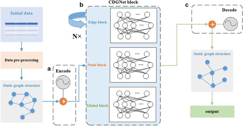
www.nature.com/scientificreports/
In this work, we simulated the self-driven collective motion under different noise and density according to
icsek32. Through simulation we find that the motion state of the collective is accompanied by
the principle of V
the generation and change of clusters, so we propose a cluster order parameter k, that is, the number of clusters
divided in the collective, to quantify the degree of synchronization of the system. Obviously, the self-driven multi-
individual system forms a dynamic network, and some basic concepts in graph theory are helpful for problem
analysis. We processed simulated data into a graph structure and constructed the Collective Dynamics Graph
network (CDGNet) model, which uses graph networks21 to reason about objects and relationships in self-driven
collective systems, so as to accomplish long-term prediction of system order parameters. The advantage is that
it fully considers the relationship between individuals and neighbors from the perspective of network topology.
Results
Data generation. The Vicsek model32 is a mathematical model used to describe active matter, which exhib-
its collective motion under higher particle density or lower noise. According to the rules of the Vicsek model,
we use MATLAB to design iterative procedures to simulate the self-driven collective dynamics of N = 4000
particles in a box with two-dimensional periodic boundary conditions. We set its initial speed to 0.03, ρ=4, and
the noise η changes from 0 to 5. η represents the disturbance in the environment, which will affect the direction
update of particles, see “Methods” section for details. At the same time, we simulated the initial speed of 0.03, η
=2, and the change of density from 0.1 to 10 to analyze the influence of noise and density on order parameters
respectively.
Further, in order to train the CDGnet model, we choose the case where N = 4000, ρ=4, and η=0.1, 1.5, 2.5,
3.5, 5. Our goal is to train the model under five noise points, covering different noise and time steps. For each
point, we generate 100 independent configurations as training examples of the network and augmented the data,
followed by generating a test set of 100 independent configurations to evaluate the model. In each independ-
ent data set, we use different initial particle positions and initial motion angles to simulate the motion of the
self-driven collective, and obtain the particle position and motion angle after each iteration. The total number
of iterations under different noise points is determined by the time it takes the system to reach a steady state.
A new cluster order parameter. It can be seen from the update formula of the Vicsek model that noise
and density are two important factors that affect the evolution of the collective, whose definition is detailed in
“Methods” section. Therefore, in order to study the evolutionary behavior of the self-driven collective system, we
simulated the conditions of different densities and noises, and got some meaningful results.
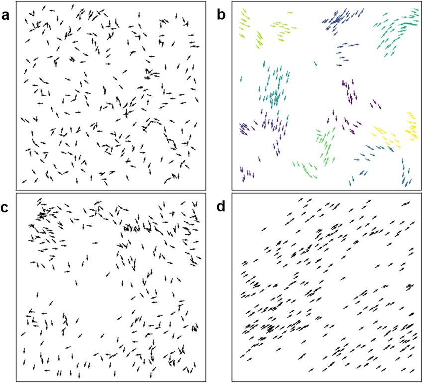
In Fig. 1a–d, the location and speed information during collective evolution is presented by setting different
densities and noises. (a) At the initial moment, individuals are randomly distributed on a two-dimensional plane
and move in random directions, and the entire collective exhibits a disordered state. (b) For low density and low
noise, small clusters moving in random directions are formed in the collective. (c) In the case of high density
and high noise, random motions with a certain correlation appear among the particles. (d) At low noise and
high density, the collective has obtained meaningful results after evolution which is that all individuals move in
the same direction. That is to say, the individuals in the collective will eventually reach synchronization after a
finite movement time (convergence time).
In the simulation, we found that some clusters will be formed during the evolution of the collective. How
to divide clusters is an important research question. How to divide clusters is an important research question.
Peruani et al.35 define the two neighboring individuals as members of the same cluster if their centers of mass
is less than R, and their motion directions differ by less than the angle α. This method relies on the choice of
parameters R and α for the definition of clusters. Different parameter combinations will lead to different results,
and the process of parameter selection is more complicated. Chen et al.36 used the Canny-Deriche algorithm
detect the boundaries of cell clusters in clustering images, and divided the areas of the clusters in pixels. The
number of individuals in a cluster is the area of a cluster divided by the average area covered by a single cell. The
method does not consider the motion direction of individual when dividing clusters. Therefore, we designs an
algorithm based on the k-means algorithm to calculate the optimal number of clusters. It only needs to input
the position and motion direction information of the individuals in the system to automatically calculate the
number of clusters k. k-means is a basic algorithm for partitioning the number of known clustering categories. It
divides the spatial distance index of the research object into several subsets according to the similarity criterion,
so that the difference between the elements in the same subset is the smallest, and the difference between the
elements in the different subsets is the largest. Obviously, if the position and direction of particles in the self-
driven collective dynamics system are used for clustering, the higher the consistency of collective movement
direction and the closer the distance between particles, the smaller the difference between individuals, so the k
value should be small.
The cluster validity index is usually used to evaluate the clustering results, and the number of clusters cor-
responding to the optimal clustering results is regarded as the optimal number of clustering categories. Some
indicators have been proposed to test the effectiveness of clustering37–39. In this paper, the average contour
coefficient is used to evaluate the clustering results, whose definition is detailed in “Methods” section. The value
range of the average contour coefficient S is [− 1,1], and the closer the distance between the samples in the clus-
ter, the farther the sample distance between the clusters, the larger the average contour coefficient, the better
the clustering effect. Then, the k with the largest average contour coefficient is the optimal number of clusters.
Based on the validity index and clustering algorithm, this paper designs an algorithm to calculate the optimal
number of clusters k, see “Methods” section for details. We calculated the changes of k with noise and density
1 N
respectively, and compared and analyzed the results with traditional order parameter va = | i=1 vi |
Nv
Scientific Reports | (2022) 12:500 | https://doi.org/10.1038/s41598-021-04456-5 2
Vol:.(1234567890)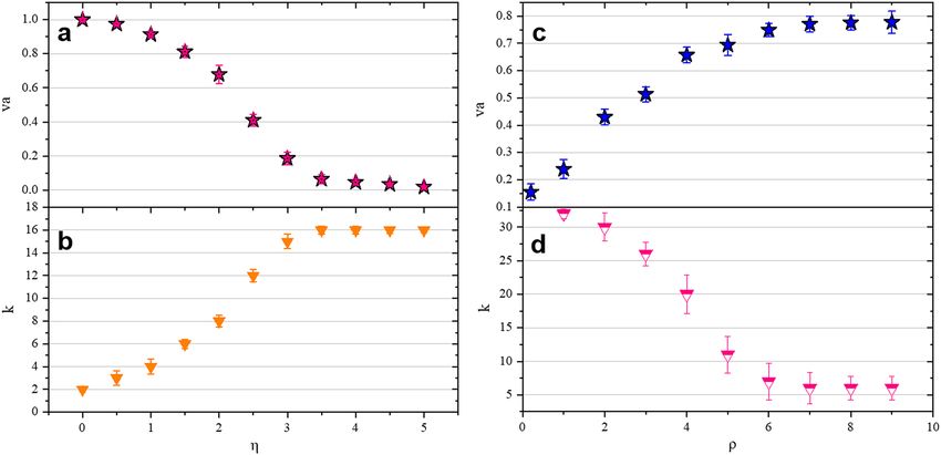
www.nature.com/scientificreports/

                                 Figure 1.  Simulation of collective motion at different densities and noises. The actual speed of the individual
                                 is indicated by a small arrow, and the tail of the arrow is the actual position of the particle. In each case, the
                                 number of particles is N = 300. (a) In the initial state of L = 7 and η = 2.0, the position and direction of the
                                 particles are random. (b) In the case of low density and low noise (L = 25, η = 0.1), the particles in the collective
                                 will aggregate after a period of time to form small clusters, where different colors indicate that the particles
                                 belong to different clusters. (c) For high-density and high-noise (L = 7, η = 2.0), the movement direction of the
                                 particles in the collective is random in a small range, but there is a certain correlation overall. (d) In the case
                                 of high density and low noise (L = 5, η = 0.1), the individuals in the collective move in the same direction. All
                                 results are obtained from simulations with a rate set to 0.03.

                                 (Fig. 2a–d). Changing the noise at a fixed density, we can observe the transition of particles from the disordered
                                 motion phase to the coherent motion phase. It can be seen from results in Fig. 2a that when the noise η in the
                                 environment gets smaller, the value of va will be closer to 1, that is, the degree of synchronization of the collective
                                 is higher. This conclusion is consistent with the assumption and analysis in Methods. As the noise increases, the
                                 degree of order decreases, that is, the system can finally reach the synchronization state only under low noise
                                 conditions. At the same time, the smaller the noise in the environment, the smaller the value of k (Fig. 2b). This
                                 is because the movement directions between particles are similar, so when the method described above is used
                                 to calculate the cluster order parameter k based on similarity criterion, the obtained value is smaller.
                                     Density is another important factor affecting the evolution of the collective. In order to find out the influence
                                 of density, we gradually increase the system density under the premise of fixed system noise and simulated box
                                 side length. In Fig. 2c,d, we show how va and k will change when the noise remains constant and the density
                                 changes. When the density of the entire system is low, va is zero, and the system is a disordered phase; when the
                                 particle density is high, va is non-zero, and the system is an ordered phase. At this time, the rotational symmetry
                                 of the system is broken and there is an overall non-zero mean pointing. It is worth noting that when the particle
                                 density is high, the similarity of the position and movement direction between particles also increases. There-
                                 fore, when the method described above is used to calculate the optimal number of clusters k based on distance

Scientific Reports |   (2022) 12:500 |                https://doi.org/10.1038/s41598-021-04456-5                                                         3

                                                                                                                                                 Vol.:(0123456789)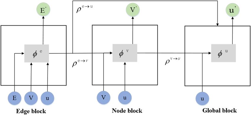
www.nature.com/scientificreports/

                                           Figure 2.  The effect of noise and density on order parameters. (a) The density is the same, (N = 4000, L = 31.6,
                                           that is, ρ = 4) the relationship between va and noise, va decreases with the increase of noise. (b) When the density
                                           is the same (N = 4000, L = 31.6, ρ = 4 can be obtained), the relationship between k and noise in the collective.
                                           When the density is constant, as the noise increases, the value of k increases accordingly. (c) In the case of
                                           constant noise (here, η = 2.0, L = 20), va increases with the increase of density. (d) When the noise is constant (η
                                           = 2.0, L = 20), the relationship between k and the density in the collective. As the density increases, the k value
                                           decreases.

                                           clustering, the obtained value is small, which is consistent with the original idea. The quantitative analysis of the
                                           noise and density in the system proves the rationality of the order parameters proposed in this paper.

                                           Prediction of order parameters under various noises. While constructing the data set, we calculated
                                           the va(k) of the system after each iteration, and trained the network of this paper to predict the change of va
                                           (k). For each training example, the positions and motion angles of N particles are put into the CDGNet model,
                                           whose definition is detailed in “Methods” section. The graph is constructed based on the distance between
                                           particles: since the field of view radius of the simulated data is 1, two particles whose distance is less than this
                                           threshold are connected by the edge. The motion angle of the particles is the attribute of the node, the relative
                                           distance between the particles is the attribute of the edge, while va(k) after each iteration is the global attrib-
                                           ute. We apply a CDGNet block to this input graph to predict va(k). The CDGNet block uses three Multi-Layer
                                           Perceptrons(MLP) to independently input the nodes, edges, and global attributes of the graph, as shown in
                                           Fig. 3b. Then, message passing on this graph, recursively update the edges, nodes, and global of the graph. The
                                           update of each edge according to the given edge, node, and global attributes, which is connected and realized
                                           through the edge MLP. Node is updated based on the given node attributes and the aggregation of its associated
                                           edge attributes, as well as the influence of global attributes. Similarly, all nodes are updated in parallel using the
                                           node MLP. Finally, global is updated through the global MLP based on the attributes of the given global and the
                                           aggregation of all nodes and edges.
                                               In the whole process of model construction, the input data is preprocessed, and the particle information in
                                           self-driven collective dynamics is transformed into a graph structure. The node, edge, and global MLPs receive
                                           attributes from the encoded graph (Fig. 3a) as input. In the CDGNet block, it is updated n times in a loop (we
                                           set n = 7) to ensure that the information of each particle is transmitted to the edge of the periodic box. The
                                           network decodes(Fig. 3c) the generated embedding into a predicted va(k), which is returned to the target va(k)
                                           via random gradient descent.
                                               With a fixed density, we predict the change of va with time in the low and high noise cases respectively. As
                                           can be seen in Fig. 4, our network achieves very good results. At a low noise level (η = 0.1), the statistical disper-
                                           sion of va is greater in the early stage of collective evolution. As the entire collective becomes stable, va fluctuates
                                           smaller and smaller, as the different simulation situations have the same law in the stable phase: va approaches 1.
                                           va changes from 0 to 1, which means that the collective has completed the transition from the disordered phase
                                           to the ordered phase. When the noise is large (η = 3.5), the statistical dispersion of the value of va in the stable
                                           phase is reduced, but it still fluctuates within a certain range. va finally stabilizes to about 0.2. It shows that in the
                                           case of high noise, the individuals in the self-driven collective will not eventually move in the same direction.
                                           After a period of evolution, the entire system can reach a relatively stable state, but the movement directions of
                                           the particles are different.

          Scientific Reports |   (2022) 12:500 |                 https://doi.org/10.1038/s41598-021-04456-5                                                        4

Vol:.(1234567890)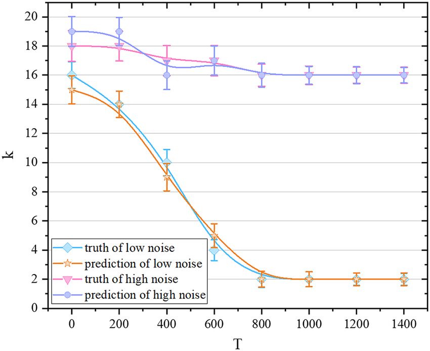
www.nature.com/scientificreports/

                                 Figure 3.  The effect of noise and density on order parameters. (a) The density is the same, (N = 4000, L = 31.6,
                                 that is, ρ = 4) the relationship between va and noise, va decreases with the increase of noise. (b) When the density
                                 is the same (N = 4000, L = 31.6, ρ = 4 can be obtained), the relationship between k and noise in the collective.
                                 When the density is constant, as the noise increases, the value of k increases accordingly. (c) In the case of
                                 constant noise (here, η = 2.0, L = 20), va increases with the increase of density. (d) When the noise is constant (η
                                 = 2.0, L = 20), the relationship between k and the density in the collective. As the density increases, the k value
                                 decreases.

                                 Figure 4.  The truth and prediction of va over time under different noises. The diamond represents the actual
                                 value of va for N = 4000, L = 31.6, η = 0.1, the pentagram represents the predicted value of va for N = 4000, L
                                 = 31.6, and η = 0.1; the square represents the actual value of va for N = 4000, L = 31.6, η = 3.5, and the inverted
                                 triangle represents the prediction value of va for N = 4000, L = 31.6, and η = 3.5.

                                     We respectively predict the cluster order parameter k at different time scales in high and low noise, as shown
                                 in Fig. 5. When the noise is small (η = 0.1), in the early stage of collective evolution, the position and movement
                                 trend of particles differ greatly between different simulation situations, which makes the standard deviation of
                                 k value larger, and the whole collective is more chaotic at this time, so the prediction accuracy of the k value
                                 will be lower than that of the stable phase. When the noise is large (η = 3.5), the prediction and truth of k will
                                 fluctuate throughout the evolution process, and the amplitude is greater than that in the case of low noise. This is
                                 because increasing the disturbance will affect the information that tends to be synchronized between the particles.
                                 However, from an overall point of view, our model can make more accurate predictions for the cluster order

Scientific Reports |   (2022) 12:500 |                https://doi.org/10.1038/s41598-021-04456-5                                                       5

                                                                                                                                                Vol.:(0123456789)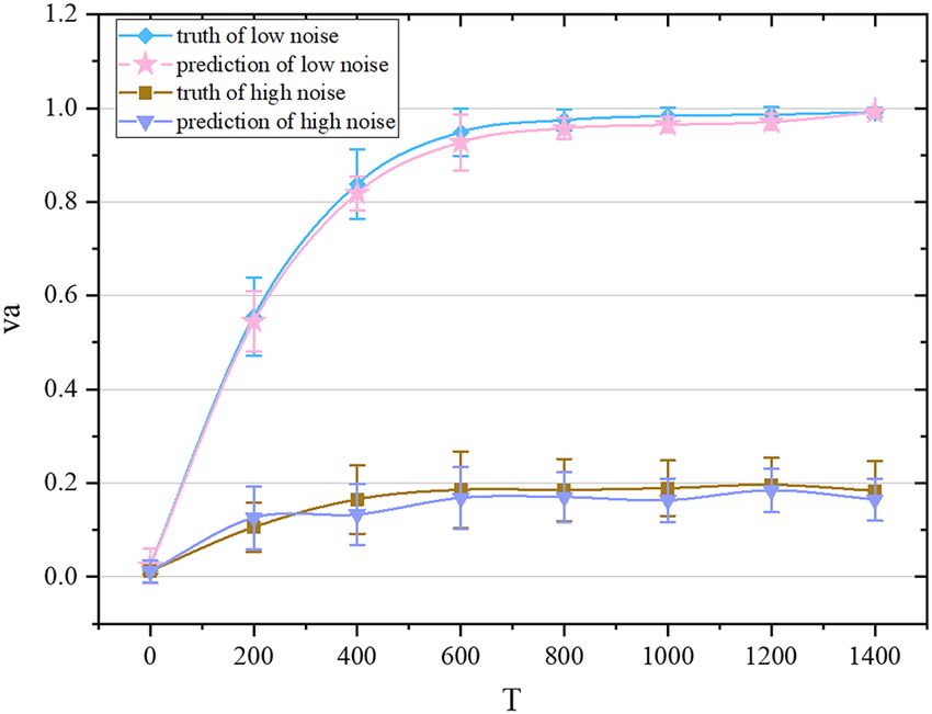
www.nature.com/scientificreports/

                                           Figure 5.  The truth and prediction of the cluster order parameter over time under different noises. The
                                           diamond represents the actual value of the cluster order parameter k when N = 4000, L = 31.6, and η = 0.1, the
                                           pentagram represents the predicted value of the cluster order parameter k when N = 4000, L = 31.6, and η = 0.1;
                                           the inverted triangle represents the actual value of the cluster order parameter k when N = 4000, L = 31.6, and η
                                           = 3.5, the circle represents the predicted value of the cluster order parameter k when N = 4000, L = 31.6, and η =
                                           3.5.

                                           Figure 6.  The truth and prediction of va varying with noise. The pentagram represents the actual value of va for
                                           N = 4000 and L = 31.6, the circle represents the predicted value of va when N = 4000 and L = 31.6.

                                           parameter of different time scales under different noise levels, so as to assess the degree of collective consistency
                                           in the evolution process.
                                               To further investigate the influence of noise on the evolution of self-driven collective, we train the model
                                           at different noise points to predict va . It can be seen that our network has a strong predictive ability, with high
                                           accuracy from low to high noise predictions, as shown in Fig. 6. Results show that the noise in the environment
                                           has a significant effect on the evolution of the self-driven collective. If there is no disturbance, the particles in
                                           the collective will move in the same direction, and the entire collective will be in a synchronized state. As the
                                           disturbance in the environment increases, the collective movement will change to a disordered phase.
                                               At the same time, we train the model under different noise conditions to predict the cluster order parameter
                                           k at steady state. Figure 7 shows that under certain noise levels, the standard deviation of the k values at stable
                                           stage is large, which reduces the prediction accuracy of the model. However, as a whole, our model can make
                                           accurate predictions of the cluster order parameter under different noise to evaluate the degree of during syn-
                                           chronization during the phase transition.

          Scientific Reports |   (2022) 12:500 |                https://doi.org/10.1038/s41598-021-04456-5                                                    6

Vol:.(1234567890)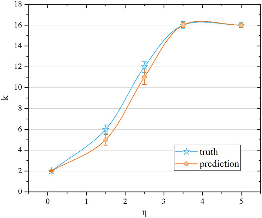
www.nature.com/scientificreports/
Figure 7. The truth and prediction of k varying with noise. The pentagram represents the actual value of k
when N = 4000 and L = 31.6, the circle represents the predicted value of k when N = 4000 and L = 31.6.
Discussion
The formation of clusters is a very meaningful phenomenon in the process of collective evolution, in recent
years, the research of aggregation phenomenon in collective dynamics has attracted many a ttention40,41. In the
process of simulating the Vicsek model, we found that the change of collective state will be accompanied by the
generation and change of clusters. Therefore, it is expected that the number of clusters can be used to describe the
phase transition of the collective. This paper proposes cluster order parameter k, and have proved the rationality
of k through quantitative analysis.
In some cases, compared with the traditional va , the cluster order parameter k has more advantages. One is
that the cluster order parameter k is calculated based on the k-means method in machine learning. The algorithm
uses the information of particle position and movement direction, and divides the particles in the system into
k sets according to the similarity criterion. This way of describing the collective phase transition is more intui-
tive, as shown in Fig. 1b. The second is that the cluster order parameter k can distinguish the collective state in
some special cases. such as Fig. 1b,c in the paper. These two figures are the movement conditions of the collec-
tive in different environment. Obviously, the aggregation of them shows different characteristics. The system in
Fig. 1b appears as small clusters, while the particles in Fig. 1c move randomly over a small area, but with some
overall correlation, forming a large cluster. These differences cannot be shown through va , which focuses more
on quantifying the uniformity of the motion direction of the system. The closer to 1 the higher the degree of
synchronization of all particles. However, by calculating k, the number of clusters in the system can be obtained,
so as to distinguish collective states with different characteristics.
At the same time, we built a graph network model based on deep learning to achieve long-term prediction
of self-driven collective dynamics, taking advantage of the structure hidden in the local neighborhoods of the
particles, and training the model by learning the interactions between the particles to predict the values of the
order parameter. In this way, it is possible to quickly predict the order parameters of the collective without
simulating the dynamics of the self-driven collective, thereby quantifying the degree of synchronization of the
entire collective.
In conclusion, we believe that this work shows the potential of using graph network methods for explora-
tion in the field of soft matter. In addition to the formation of dynamic clusters, many other dynamic patterns
have been formed in the active matter system, such as dynamic h yperuniform42–44 and motility-induced phase
45,46
separation , which is the direction we will explore in future work.
Methods
Vicsek model. In the Vicsek model32,N individuals that can be regarded as mass points move at the same
rate on the plane of the L ∗ L two-dimensional periodic boundary condition. At the initial moment, the position
of each individual is randomly distributed in the plane area, and the direction of the movement of each indi-
vidual is randomly distributed between [−π, π).
At each time t + 1, the angle of each individual is updated according to the vector average of the neighbor
angles, and some random disturbances (η) are added. The neighbors of an individual i consist of individuals
centered at the current position of that individual and whose distance from that individual is less than the radius
r of the field of view.
Each individual always moves at a constant rate v in the plane, so the equation for position change is:
xi (t + 1) = xi (t) + vcosθi (t)�t
yi (t + 1) = yi (t) + vsinθi (t)�t
i = 1, 2, . . . , N (1)
Scientific Reports | (2022) 12:500 | https://doi.org/10.1038/s41598-021-04456-5 7
Vol.:(0123456789)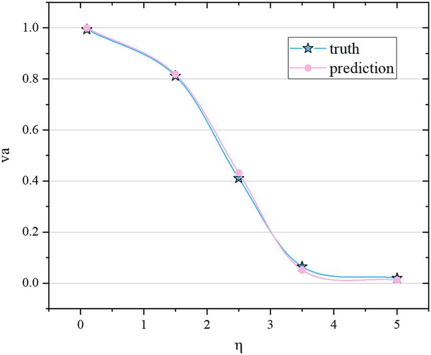
www.nature.com/scientificreports/
where θi (t) is the angle at which individual i moves at moment t, and its update rule is:
θi (t + 1) =< θi (t) >r +�θ (2)
where �θ represents the random number chosen with uniform probability from the interval [−η/2, η/2], and η
represents the noise in the environment. < θi (t) >r is the average movement direction of all individuals (includ-
ing individual i itself) within the field of view radius r with individual i as the center. It is calculated by the fol-
lowing formula:
−1
j∈Ni (t)
sinθj (t)
< θi (t) >r = tan (3)
j∈Ni (t) cosθj (t)
Where Ni (t) represent the neighbor of individual i at time t.
To analyze the synchronization of the model, Vicsek et al. define an order parameter called the absolute value
of the average normalized velocity, denoted by va , which is defined as:
N
1
va = | vi | (4)
Nv
i=1
In this way, va can be used to characterize the degree of synchronization of all individuals in the collective. If
after several time steps, all individuals in the collective reach a synchronized state, the value of va approaches
1 at this time; if the movement direction of all individuals in the collective is random, then the value of va is
approximately 0. Obviously, 0≤ va ≤1, larger values indicate greater consistency in the direction of individual
movement. When va = 1, all individuals move in the same direction.
Definition of the average contour coefficient. The contour coefficient of a sample point Xi is defined
as follows:
b−a
Si = (5)
max(a, b)
where a is the average distance between Xi and other samples in the same cluster, called the cohesion degree,
and b is the average distance between Xi and all samples in the nearest cluster, called the separation degree. The
definition of Xi ’s nearest cluster is as follows:
1
Cj = arg min | p − Xi |2 (6)
Ck npǫCk
where p is a sample in a certain cluster Ck , and n is the number of samples in Ck . In fact, after using the average
distance of Xi to all samples of a certain cluster as a measure of the distance from the point to the cluster, the
cluster with the smallest distance from Xi is selected as the closest cluster.
After calculating the contour coefficients of all samples, average the contour coefficients to obtain the average
contour coefficient. Calculated as follows:
n
1
S= Si . (7)
n
i=1
Algorithm for finding the optimal number of clusters. The search range of the number of clusters
is [kmin , kmax ], kmin=1 means that the sample is evenly distributed without obvious feature differences. Usually,
√
the minimum number of clusters is 2. For how to determine kmax , most scholars use empirical rules38: k ≤ n.
The average contour coefficient index described above has a good test performance due to its simple structure
and low computational complexity. Based on this, this paper designs a spatial clustering k-value optimization
algorithm. The algorithm process is described as follows:
Algorithm: Based on the k-means algorithm, the optimal k value is calculated by the average contour
coefficient.
Input: Data containing n objects.
Output: k value under the maximum condition of the average contour coefficient.
Algorithm steps:
√
(1) Calculate the upper bound of the optimal solution k ≤ n; √
(2) Use the k-means algorithm to achieve spatial clustering under all numbers when k ≤ n , where the
position and direction of the particles are used as the feature vector of k-means clustering, feature list =
[ x, y, vx , vy].;
(3) Calculate the S value under different cluster numbers k according to the average contour coefficient method;
(4) Search for the largest average contour coefficient S, and write down the corresponding k;
(5) End.
Scientific Reports | (2022) 12:500 | https://doi.org/10.1038/s41598-021-04456-5 8
Vol:.(1234567890)www.nature.com/scientificreports/
Figure 8. The basic building blocks of a graph network. It is divided into three main blocks: edge, node, and
global. Information is disseminated and updated through certain rules.
The CDGNet model. Graph networks21, a generic modular framework for deep learning, can be viewed as
a superset of previous graph-based neural networks. The advantage of GN is its versatility, allowing it to be used
for analysis if the structure of the target problem can be encoded in the form of a graph, or if a priori knowledge
of the relationships between input entities can itself be described as a graph. GN also has strong combination and
generalization capabilities. The GN block supports depth or recursive arrangement. Information can be propa-
gated across the graph network to allow more information to perform computations and complex functions. At
the same time, the calculation is not performed at the macro level of the entire system but is multiplexed across
entities and relationships, which enables the network to have a good fitting result for unknown data sets. Here,
we will outline the implementation of the CDGNet model for a self-driven collective.
GN is a graph-to-graph function which can be represented by G = (u, V , E), with V, E, and u for the node
(individuals), edge (effects between individuals), and global attributes respectively. For a self-driven collective
system, this graph is constructed based on the distance between individuals, and edges are defined by the relative
distance between particles. The set of nodes is V = {vi }i=1:N v , where vi denotes the attribute of the ith node, N v is
the number of nodes. The set of edges is E = {(ek , rk , sk )}k=1:N e , where ek represents the attribute of the kth edge,
rk and sk are the indexes of the nodes connected by the kth edge, which are the receiving node and the sending
node respectively, and N e is the number of edges.
A GN block contains three blocks: edge, node, and global. These blocks can be composed of deep or recur-
rent neural network configurations. The blocks are related through certain rules to update the graph, as shown
in Fig. 8. It includes six internal functions, three update functions, and three aggregate functions.
The update rules for the GN block are as follows:
First, the edge block calculates an output ek′ for each edge, and updates it with attributes from itself, its con-
nected individuals (with indexes vrk and vsk ), and the global attribute u, as follows:
ek′ = φ e (ek , vrk , vsk , u) (8)
Among them, is the update function of the edges. Next, for each node, the node block aggregates all edges
φe
pointing to it into ēi′ , as follows:
ēi′ = ρ e→v (Ei′ ) (9)
where ρ e→v is the aggregate function of directed edges pointing to each receiving node, Ei′
= {(ek′ , rk , sk )}rk =i,k=1:N e
is the set of all directed edges pointing to the node with index i.
Then the output vi′ of each node is calculated. The attributes of each node use its own attributes, the edges
connected to it, and the global attribute u to update:
vi′ = φ v (ēi′ , vi , u) (10)
Among them, φ v is the update function of the node.
Finally, in the global block, the output at the edge and node levels are aggregated to calculate global attributes:
ē′ =ρ e→u (E ′ ) (11)
v̄ ′ =ρ v→u (V ′ ) (12)
Scientific Reports | (2022) 12:500 | https://doi.org/10.1038/s41598-021-04456-5 9
Vol.:(0123456789)www.nature.com/scientificreports/
u′ =φ u (ē′ , v̄ ′ , u) (13)
Among them, ρ e→u is the aggregate function of all edges on the graph, all the updated edges are aggregated into
ē′ , where E ′ = {(ek′ , rk , sk )}k=1:N e . ρ v→u is the aggregate function of all nodes on the graph, which aggregates
all updated nodes as v̄ ′ , where V ′ = {vi ′ }i=1:N v . φ u is the update function of the global attributes. Therefore, the
output of GN is the collection of all edge, node and graph-level attributes, G′ = (u′ , V ′ , E ′ ).
The choice of update function φ e, φ v and φ u directly determines the performance of the model in actual tasks.
In the CDGNet model, we chose Multi-Layer Perceptron (MLP) as the update function as shown in Fig. 3b. For
feature extraction and data downscaling, an encoder was added to preprocess the inputs before the CDGNet
block. It is found that this method improves the training speed and accuracy of the model. In the CDGNet block,
three multilayer perceptrons are used to update node, edge and global attributes, respectively. The CDGNet block
loops n times to implement complex calculations, and the processed information is decoded with a decoder
into the desired form. The encoder compresses the input into the latent space representation, which can be
represented by the function f(x), and the decoder reconstructs the latent space representation into the output,
which can be represented by the function g(x), the encoding function f(x) and the decoding function g(x) are
all neural network models.
Received: 21 July 2021; Accepted: 16 December 2021
References
1. Hannun, A. et al. Deep speech: Scaling up end-to-end speech recognition. arXiv preprint arXiv:1412.5567 (2014).
2. Wu, Y. et al. Google’s neural machine translation system: Bridging the gap between human and machine translation. arXiv preprint
arXiv:1609.08144 (2016).
3. Mehta, P. et al. A high-bias, low-variance introduction to machine learning for physicists. Phys. Rep. 810, 1–124 (2019).
4. Sarma, S. D., Deng, D. -L. & Duan, L. -M. Machine learning meets quantum physics. arXiv preprint arXiv:1903.03516 (2019).
5. Brunton, S. L., Noack, B. R. & Koumoutsakos, P. Machine learning for fluid mechanics. Annu. Rev. Fluid Mech. 52, 477–508 (2020).
6. Chen, C., Ye, W., Zuo, Y., Zheng, C. & Ong, S. P. Graph networks as a universal machine learning framework for molecules and
crystals. Chem. Mater. 31, 3564–3572 (2019).
7. Webb, S. Deep learning for biology. Nature 554, 555–558 (2018).
8. Muinos-Landin, S., Ghazi-Zahedi, K. & Cichos, F. Reinforcement learning of artificial microswimmers. arXiv preprint arXiv:1 803.
06425 (2018).
9. Aviv, R. et al. The human cell atlas. Elife 6, e27041 (2017).
10. Bo, S., Schmidt, F., Eichhorn, R. & Volpe, G. Measurement of anomalous diffusion using recurrent neural networks. Phys. Rev. E
100, 010102 (2019).
11. Muñoz-Gil, G., Garcia-March, M. A., Manzo, C., Martín-Guerrero, J. D. & Lewenstein, M. Single trajectory characterization via
machine learning. New J. Phys. 22, 013010 (2020).
12. Hannel, M. D., Abdulali, A., O’Brien, M. & Grier, D. G. Machine-learning techniques for fast and accurate feature localization in
holograms of colloidal particles. Opt. Express 26, 15221–15231 (2018).
13. Newby, J. M., Schaefer, A. M., Lee, P. T., Forest, M. G. & Lai, S. K. Convolutional neural networks automate detection for tracking
of submicron-scale particles in 2D and 3D. Proc. Natl. Acad. Sci. 115, 9026–9031 (2018).
14. Lukeman, R., Li, Y.-X. & Edelstein-Keshet, L. Inferring individual rules from collective behavior. Proc. Natl. Acad. Sci. 107,
12576–12580 (2010).
15. Budrene, E. O. & Berg, H. C. Dynamics of formation of symmetrical patterns by chemotactic bacteria. Nature 376, 49–53 (1995).
16. Ballerini, M. et al. Interaction ruling animal collective behavior depends on topological rather than metric distance: Evidence
from a field study. Proc. Natl. Acad. Sci. 105, 1232–1237 (2008).
17. Buhl, J. et al. From disorder to order in marching locusts. Science 312, 1402–1406 (2006).
18. Fowler, J. H. & Christakis, N. A. Cooperative behavior cascades in human social networks. Proc. Natl. Acad. Sci. U. S. A. 107,
5334–5338. https://doi.org/10.1073/pnas.0913149107 (2010).
19. Gazzola, M., Tchieu, A. A., Alexeev, D., de Brauer, A. & Koumoutsakos, P. Learning to school in the presence of hydrodynamic
interactions. J. Fluid Mech. 789, 726–749 (2016).
20. Verma, S., Novati, G. & Koumoutsakos, P. Efficient collective swimming by harnessing vortices through deep reinforcement learn-
ing. Proc. Natl. Acad. Sci. 115, 5849–5854 (2018).
21. Battaglia, P. W. et al. Relational inductive biases, deep learning, and graph networks. arXiv preprint arXiv:1806.01261 (2018).
22. Sanchez-Gonzalez, A. et al. Graph networks as learnable physics engines for inference and control. arXiv preprint arXiv:1806.
01242 (2018).
23. Sanchez-Gonzalez, A. et al. Learning to simulate complex physics with graph networks. arXiv preprint arXiv:2002.09405 (2020).
24. Battaglia, P., Pascanu, R., Lai, M. & Rezende, D. J. in Advances in Neural Information Processing Systems. Interaction networks for
learning about objects, relations and physics. 4502–4510.
25. Sun, C., Karlsson, P., Wu, J., Tenenbaum, J. B. & Murphy, K. Stochastic prediction of multi-agent interactions from partial observa-
tions. arXiv preprint arXiv:1902.09641 (2019).
26. Bapst, V. et al. Structured agents for physical construction. arXiv preprint arXiv:1904.03177 (2019).
27. Li, Y. et al. in 2019 International Conference on Robotics and Automation (ICRA) 1205–1211 (IEEE).
28. Kossen, J., Stelzner, K., Hussing, M., Voelcker, C. & Kersting, K. Structured object-aware physics prediction for video modeling
and planning. arXiv preprint arXiv:1910.02425 (2019).
29. Bapst, V. et al. Unveiling the predictive power of static structure in glassy systems. Nat. Phys. 16, 448–454 (2020).
30. Qasim, S. R., Kieseler, J., Iiyama, Y. & Pierini, M. Learning representations of irregular particle-detector geometry with distance-
weighted graph networks. Eur. Phys. J. C 79, 1–11 (2019).
31. Iiyama, Y. et al. Distance-weighted graph neural networks on FPGAs for real-time particle reconstruction in high energy physics.
arXiv preprint arXiv:2008.03601 (2020).
32. Vicsek, T., Czirok, A., Ben-Jacob, E., Cohen, I. I. & Shochet, O. Novel type of phase transition in a system of self-driven particles.
Phys. Rev. Lett. 75, 1226–1229. https://doi.org/10.1103/PhysRevLett.75.1226 (1995).
33. Barberis, L. & Albano, E. V. Evidence of a robust universality class in the critical behavior of self-propelled agents: Metric versus
topological interactions. Phys. Rev. E 89, 012139 (2014).
Scientific Reports | (2022) 12:500 | https://doi.org/10.1038/s41598-021-04456-5 10
Vol:.(1234567890)www.nature.com/scientificreports/
34. Shang, Y. & Bouffanais, R. Consensus reaching in swarms ruled by a hybrid metric-topological distance. Eur. Phys. J. B 87, 294
(2014).
35. Peruani, F., Starruss, J., Jakovljevic, V., Sgaard-Andersen, L. & Br, M. Collective motion and nonequilibrium cluster formation in
colonies of gliding bacteria. Phys. Rev. Lett. 108, 098102 (2012).
36. Chen, X., Dong, X., Be’Er, A., Swinney, H. & Zhang, H. Scale-invariant correlations in dynamic bacterial clusters. Phys. Rev. Lett.
108, 148101 (2012).
37. Bezdek, J. C. & Pal, N. R. Some new indexes of cluster validity. IEEE Trans. Syst. Man Cybern. Part B (Cybern.) 28, 301–315 (1998).
38. Rezaee, M. R., Lelieveldt, B. B. F. & Reiber, J. H. C. A New Cluster Validity Index for the Fuzzy c-Mean. (Elsevier Science Inc., 1998).
39. Dudoit, S. & Fridlyand, J. A prediction-based resampling method for estimating the number of clusters in a dataset. Genome Biol.
Res. 3, 1–21 (2002).
40. Barberis, L. & Peruani, F. Large-scale patterns in a minimal cognitive flocking model: Incidental leaders, nematic patterns, and
aggregates. Phys. Rev. Lett. 117, 248001 (2016).
41. Gustavsson, K., Berglund, F., Jonsson, P. & Mehlig, B. Preferential sampling and small-scale clustering of gyrotactic microswim-
mers in turbulence. Phys. Rev. Lett. 116, 108104 (2016).
42. Hexner, D. & Levine, D. Noise, diffusion, and hyperuniformity. Phys. Rev. Lett. 118, 020601 (2017).
43. Lei, Q.-L., Ciamarra, M. P. & Ni, R. Nonequilibrium strongly hyperuniform fluids of circle active particles with large local density
fluctuations. Sci. Adv. 5, eaau7423 (2019).
44. Lei, Q.-L. & Ni, R. Hydrodynamics of random-organizing hyperuniform fluids. Proc. Natl. Acad. Sci. 116, 22983–22989 (2019).
45. Cates, M. E. & Tailleur, J. Motility-induced phase separation. Annu. Rev. Condens. Matter Phys. 6, 219–244 (2015).
46. Ma, Z., Yang, M. & Ni, R. Dynamic assembly of active colloids: Theory and simulation. Adv. Theory Simul. 3, 2000021 (2020).
Acknowledgements
Thanks to Prof. Mingcheng Yang for the helpful discussion. This work is supported by National Natural Science
Foundation of China Grants No. 11702289, Key core tech-nology and generic technology research and devel-
opmentproject of Shanxi Prowince, No. 2020XXX013 and National Key Research and Development Project.
Author contributions
R.W., F.F., and W.Z. designed the project. J.C. generated data set and supplemented some experiments. R.W.
analyzed the data and constructed a predictive model. F.F. optimized the model parameters. R.W., F.F. and W.Z.
wrote the paper. R.W. and J.C. prepared figures. All authors reviewed the manuscript.
Competing interests
The authors declare no competing interests.
Additional information
Supplementary Information The online version contains supplementary material available at https://doi.org/
10.1038/s41598-021-04456-5.
Correspondence and requests for materials should be addressed to W.Z.
Reprints and permissions information is available at www.nature.com/reprints.
Publisher’s note Springer Nature remains neutral with regard to jurisdictional claims in published maps and
institutional affiliations.
Open Access This article is licensed under a Creative Commons Attribution 4.0 International
License, which permits use, sharing, adaptation, distribution and reproduction in any medium or
format, as long as you give appropriate credit to the original author(s) and the source, provide a link to the
Creative Commons licence, and indicate if changes were made. The images or other third party material in this
article are included in the article’s Creative Commons licence, unless indicated otherwise in a credit line to the
material. If material is not included in the article’s Creative Commons licence and your intended use is not
permitted by statutory regulation or exceeds the permitted use, you will need to obtain permission directly from
the copyright holder. To view a copy of this licence, visit http://creativecommons.org/licenses/by/4.0/.
© The Author(s) 2022
Scientific Reports | (2022) 12:500 | https://doi.org/10.1038/s41598-021-04456-5 11
Vol.:(0123456789)You can also read