LEARNED IMAGE CODING FOR MACHINES: A CONTENT-ADAPTIVE APPROACH
←
→
Page content transcription
If your browser does not render page correctly, please read the page content below
LEARNED IMAGE CODING FOR MACHINES: A CONTENT-ADAPTIVE APPROACH

                                                             Nam Le∗† , Honglei Zhang† , Francesco Cricri† , Ramin Ghaznavi-Youvalari† ,
                                                                            Hamed Rezazadegan Tavakoli† , Esa Rahtu∗
                                                                                 †
                                                                                     Nokia Technologies, ∗ Tampere University
                                                                                               Tampere, Finland
arXiv:2108.09992v3 [eess.IV] 13 Oct 2021

                                                                   ABSTRACT                                  called Video coding for machines (VCM) [3] in the effort to
                                                                                                             study and standardize these use cases.
                                           Today, according to the Cisco Annual Internet Report (2018-            In response to this emerging challenge, many studies have
                                           2023), the fastest-growing category of Internet traffic is        been actively conducted to explore alternative coding solu-
                                           machine-to-machine communication. In particular, machine-         tions for the new use cases. There exist mainly two categories
                                           to-machine communication of images and videos represents          of solutions: adapting the traditional image and video codecs
                                           a new challenge and opens up new perspectives in the context      for machine-consumption [4, 5], and employing end-to-end
                                           of data compression. One possible solution approach consists      learned codecs that are optimized directly for machines by
                                           of adapting current human-targeted image and video cod-           taking advantage of the neural network (NN) based solutions
                                           ing standards to the use case of machine consumption. An-         [6, 7]. Each approach has its own pros and cons. Traditional
                                           other approach consists of developing completely new com-         video codec-based solutions, built upon mature technologies
                                           pression paradigms and architectures for machine-to-machine       and broadly adopted standards, are often compatible with ex-
                                           communications. In this paper, we focus on image com-             isting systems [4, 5]. However, it is difficult to optimize the
                                           pression and present an inference-time content-adaptive fine-     overall performance of a system that consists of a traditional
                                           tuning scheme that optimizes the latent representation of an      video codec and neural networks that perform machine tasks
                                           end-to-end learned image codec, aimed at improving the            [6]. On the other hand, NN-based codecs are easier to opti-
                                           compression efficiency for machine-consumption. The con-          mize, though they may suffer from data domain shift at in-
                                           ducted experiments targeting instance segmentation task net-      ference time, when the test data distribution differs from the
                                           work show that our online finetuning brings an average bitrate    distribution of the data used for training the learnable param-
                                           saving (BD-rate) of -3.66% with respect to our pretrained         eters.
                                           image codec. In particular, at low bitrate points, our pro-
                                                                                                                  In this work, we address the problem of domain shift at in-
                                           posed method results in a significant bitrate saving of -9.85%.
                                                                                                             ference time for end-to-end learned NN-based solutions. We
                                           Overall, our pretrained-and-then-finetuned system achieves -
                                                                                                             propose a content-adaptive fine-tuning technique that can en-
                                           30.54% BD-rate over the state-of-the-art image/video codec
                                                                                                             hance the coding efficiency on-the-fly at the inference stage
                                           Versatile Video Coding (VVC) on instance segmentation.
                                                                                                             without modifying the architecture or the learned parameters
                                               Index Terms— Image coding for machines, learned im-           of the codec. We demonstrate that the proposed method, as
                                           age compression, content-adaptation, finetuning, video cod-       a complementary process, can improve the performance of a
                                           ing for machines                                                  learned image codec targeting instance segmentation by sav-
                                                                                                             ing up to -9.85% in bitrate.

                                                              1. INTRODUCTION
                                                                                                                                2. RELATED WORK
                                           It is predicted that half of global connected devices and con-
                                           nections will be for machines-to-machine (M2M) commu-             End-to-end learned approaches aimed at improving the task
                                           nications by 2023 [1]. There has been a tremendous im-            performance on the outputs of the codec, have been studied
                                           provement of coding efficiency in the recent iterations of        in some recent works. Learned codecs that are optimized
                                           the human-oriented video coding standards such as Versatile       for both human and machine consumption are proposed in
                                           Video Coding (VVC) [2]. The performance of such codecs,           [8] and [7], either by integrating the semantic features into
                                           however, remains questionable in the use cases where non-         the bitstream [8] or by adapting the targeted task networks
                                           human agents, hereinafter machines, are the first-class con-      to the learned latent representation [7]. Concentrating solely
                                           sumers. To understand this problem, the Moving Picture Ex-        on machine-consumption use cases, the codecs presented in
                                           perts Group (MPEG) has recently issued a new Ad-hoc group         [6] achieve state-of-the-art coding performance without any
modifications to the task networks. The above methods im-                                                                                Receiver side
prove the task performance by designing new codecs trained                                           Probability
                                                                                                       model
on a certain amount of training data, which may have a dif-
ferent distribution than that of the test data at inference time.                                    bitstream
                                                                                         EE                            ED         Predictions
Our proposed method adapts only the transmitted data to the
input content, hence alleviating the data domain shift while
the codec remains unchanged.                                                                                                          Task network
     Inference-time finetuning schemes have already been ex-
plored in numerous works in the context of image compres-
                                                                        Input image                                Output image
sion. The goal is to optimize some parts of the codec in order
to maximize its performance on the given input test data. This
operation is performed on the encoder side, and the subject of
optimization may be the encoder itself, the output of the en-        Fig. 1. System architecture of the baseline Image Coding for
coder, or the decoder. In [9, 10], the post-processing filter        Machines system. “EE” and “ED” denote arithmetic entropy
is finetuned at decoder side by using weight-updates signaled        encoder and decoder, respectively.
from the encoder to the decoder at inference time. Techniques
of latent tensor overfitting for better human consumption are
presented in [11, 12], aiming at reducing the distortion in the      sion rate. For each level of downsampling, the probabil-
pixel domain. Such approaches are useful for enhancing the           ity model learns the conditional distributions p(z (l) |z (l+1) ),
fidelity in the pixel domain and their application is straightfor-   where z (l+1) denotes the downsampled image by a factor of 2
ward, as the ground-truth at the encoder-side is readily avail-      of z (l) , and l ∈ [1, N ]. The bitstream at each level is coded us-
able (the uncompressed image itself). However, similar tech-         ing the corresponding predicted conditional distribution with
niques are not directly applicable to a NN-based codec that          the lower resolution image as the context. These bitstreams
targets machine tasks, where neither the ground-truth nor the        can perfectly reconstruct z (1) from z (N ) . We apply this cod-
task networks are available at the encoder side. In this pa-         ing pipeline to losslessly compress the quantized latent ŷ in
per, we propose a content-adaptive finetuning technique that         our base ICM system. The bitrate of the coded bitstream is
can further improve the performance of a NN-based codec for          estimated by the Shannon cross-entropy:
machine consumption.
                                                                                      Lrate = Eŷ∼mŷ [− log2 pŷ (ŷ)] ,                            (1)
                 3. PROPOSED METHOD                                  where mŷ denotes the true distribution of input tensor ŷ and
                                                                     pŷ (ŷ) denotes the predicted distribution of ŷ.
An image coding for machines (ICM) codec aims to achieve                  Task network is based on Mask R-CNN [14] for instance
optimal task network performance given a targeted bitrate, as        segmentation. This network is pre-trained and kept unmodi-
opposed to the traditional codecs which are optimized for the        fied in our experiments. It provides predictions for task per-
visual quality. In this work, we propose a content-adaptive          formance evaluation and task loss Ltask during the training
finetuning scheme that further enhances the coding efficiency        of the codec. The task loss is defined as the training loss of
of NN-based ICM codecs. As a concrete example, we apply              the Mask R-CNN network:
this technique on a baseline ICM codec described below.
                                                                         Ltask = Lcls + Lreg + Lpreg + Lobj + Lmask ,                                (2)
                                                                                 |    {z   } |      {z    }   | {z }
3.1. Baseline ICM system                                                              classifier branch       RPN branch          mask branch

We use an ICM system based on [6] as a baseline. Such sys-           where Lcls , Lreg , Lpreg , Lobj and Lmask denote classifica-
tem consists of three main components: a probability model,          tion loss, regression loss, region proposal regression loss, ob-
a task network representing the “machine”, and an autoen-            jectness loss and mask prediction loss, respectively. These
coder. The overview of this system is presented in Fig. 1.           losses come from the 3 branches of the network architecture:
To simplify the experiments, while still following the same          classifier branch, region proposal network (RPN) branch, and
principles proposed in [6], our system has some architectural        mask predictor branch, respectively. Readers are referred to
adjustments which are described in the next paragraphs.              [14] for further information about these components.
    Probability model estimates the probability distribution             Autoencoder performs the lossy encoding and decoding
and the bitrate of the data to be compressed. Instead of the         operations. Together with the probability model and the arith-
probability model in [6], we incorporate a probability model         metic codec, it forms the “codec” in the ICM system. It
based on the method proposed for a lossless image coding             is a convolutional neural network (CNN) with residual con-
system [13], in which a N -level-downsampled version of the          nections as illustrated in Fig. 2. This is an almost identical
input image z (1) is encoded to achieve a higher compres-            network to the one described in [6], except for the number
CONV         CONV BLOCK       CONV         CONV BLOCK       CONV
               C: 64 S: 2     C: 64 S: 1     C: 64 S: 2     C: 64 S: 1     C: 8 S: 2
 Encoder

 Decoder
               TCONV         CONV BLOCK       TCONV        CONV BLOCK       TCONV                                                   Update
               C: 3 S: 2      C: 64 S: 1     C: 64 S: 2     C: 64 S: 1     C: 64 S: 2

                                   CONV

                              RES BLOCK
              PReLU                                       ReLU
                               C: 64 S: 1

           CONV                             CONV                    CONV

      BASIC   BASIC                  BASIC    BASIC                 BASIC
                             ReLU                            ReLU                   ReLU        Input image
      BLOCK   BLOCK                  BLOCK    BLOCK                 BLOCK

                                                                                                                                     Perceptual evaluation
                            CONV    ReLU     CONV    ReLU

                                                                                                  Fig. 3. Online latent tensor finetuning pipeline

Fig. 2. Auto-encoder architecture. The convolutional blocks                                decoder-side, resulting in bitrate overhead. Instead of fine-
are illustrated by sharp rectangles. “TCONV” denotes the                                   tuning the encoder, it is sufficient to finetune the latent ten-
transposed convolutional layers. In each convolutional block,                              sor y, by back-propagating gradients of the loss with respect
“S” denotes the stride and “C” denotes the number of out-                                  to elements of y through the frozen decoder and probability
put channels for all of the children blocks. These values are                              model. However, at the inference stage, Ltask is unknown to
inherited from the parent block if not stated otherwise.                                   the encoder since the ground-truth for the tasks is not avail-
                                                                                           able. Furthermore, the task network is only available on the
of channels in the last layer of the encoder. We use a 6-                                  decoder side and not on the encoder side. We hypothesize that
bit uniform quantizer in this work, denoted as Q(·). The                                   the intermediate layer features of the task networks should be
learned encoder takes the uncompressed image x as input and                                correlated to those of other vision tasks to a certain degree.
transforms it into a more compressible latent representation                               Therefore, we propose finetuning y by using the gradients of
y = E(x; θ E ), where θ E denotes the learned parameters of                                the following finetuning loss:
the encoder. The quantized latent ŷ = Q(y) is submitted to                                         L̄total = w̄rate · L̄rate + w̄proxy · L̄proxy ,          (4)
the probability model for a distribution estimation, which is
used as the prior for the entropy coding. The decoder trans-                               where w̄rate , w̄proxy denote the weights for the finetuning
forms the latent data back to the pixel domain as the recon-                               loss terms, L̄rate is similar to Lrate , and L̄proxy denotes a
structed image x̂ = D(ŷ; θ D ).                                                           feature-based perceptual loss which acts as a proxy for the
    Training strategy: the above “codec” is trained to opti-                               task loss Ltask . Fig. 3 illustrates our finetuning scheme. In
mize the multi-task loss function:                                                         our experiments, we used a VGG-16 [15] model pretrained
                                                                                           on ImageNet [16] as the feature extractor. The perceptual loss
 Ltrain = wrate · Lrate + wtask · Ltask + wmse · Lmse , (3)                                term L̄proxy is given by
where Lrate and Ltask are specified by Eq. (1) and Eq. (2),                                  L̄proxy = MSE(F2 (x), F2 (x̂)) + MSE(F4 (x), F4 (x̂)),
Lmse denotes the mean square error between x and x̂, and                                                                                              (5)
wrate , wtask , wmse are the scalar weights for the above                                  where MSE denotes the mean square error calculation and
losses, respectively. These values follow the same configu-                                Fi (t) denotes the input of the ith Max Pooling layer of the
ration proposed in [6], in order to delicately handle the loss                             feature extractor given the input t. The feature extraction is
terms balancing problem and at the same time train the codec                               visualized in Fig. 4. The finetuning process is described by
to achieve good efficiency on a wide variety of targeted bi-                               algorithm 1. By using the gradients from L̄total w.r.t y, the
trates.                                                                                    system learns to update y for better coding efficiency without
                                                                                           the knowledge of the task network or ground-truth annota-
3.2. Online latent tensor finetuning                                                       tions, which makes it a sensible solution.

At the inference stage, it is possible to further optimize the
                                                                                                               4. EXPERIMENTS
system by adapting it to the content being encoded. This way,
even better rate-task performance trade-offs can be achieved.
                                                                                           4.1. Experimental setup
However, this content-adaptive optimization should be done
only for the components at the encoder-side, otherwise addi-                               For the baseline system, we followed the same training setup
tional signals containing the updates need to be sent to the                               as in [6]. We used Cityscapes dataset [17] which contains
Algorithm 1: Latent finetuning at inference stage
0.240
Rate-Task performance
Input: Input image x, learning rate η, number of ICM baseline
mAP (Mean average precision)
0.227 VVC full-size images
iterations n, loss weights w̄rate , w̄proxy 0.220 VVC Pareto front
Output: Content-adapted latent tensor ȳ Proposed
Uncompressed
0.200 Corresponding points
function FeatureLoss(t1 , t2 ):
return MSE(F2 (t1 ), F2 (t2 )) +
0.180
MSE(F4 (t1 ), F4 (t2 ))
0.160
ȳ = E(x)
// Finetuning iterations
0.140
for i = 1 → n do
ŷ = Q(ȳ)
0.120
pŷ = P (ŷ) 0.030 0.035 0.040 0.045 0.050 0.055 0.060 0.065
x̂ = D(ŷ) Bits per pixel
L̄rate = Eŷ∼mŷ [− log2 pŷ (ŷ)]
L̄proxy = FeatureLoss (x, x̂)
L̄total = w̄rate · L̄rate + w̄proxy · L̄proxy Fig. 5. Rate-performance curves on low bitrates. The small
ȳ = ȳ − η · ∇ȳ L̄total dashed lines connect the baseline checkpoints and their re-
end spective finetuned versions.
return ȳ
using the Shannon entropy in Eq. (1) instead of the bitrates
Conv + ReLU
Conv + ReLU
Conv + ReLU
Conv + ReLU
Conv + ReLU
Conv + ReLU
Conv + ReLU
Conv + ReLU
Conv + ReLU
Conv + ReLU
Conv + ReLU
Conv + ReLU
Conv + ReLU
Dense layers
Max Pooling
Max Pooling
Max Pooling
Max Pooling
Max Pooling
arising from the actual bitstream lengths. In practice, we have
verified that the differences between them are negligible.
We also provide evaluation results using the state-of-the-
art video codec VVC (reference software VTM-8.22 , All-intra
configuration), under JVET common test conditions [18].
The val set is coded in 28 settings of 7 quantization param-
eters (22, 27, 32, 37, 42, 47 and 52) and 4 downsampling
factors (1, 0.75, 0.50 and 0.25) to achieve different output
bitrates. The 28 coded versions of the original input are
Fig. 4. Feature extraction using VGG-16 (Eq. (5)). then evaluated for task performance. The Pareto front from
these 28 pairs of bitrate and corresponding task performance
is clipped for the relevant bitrate range and visualized in Fig. 5
uncompressed images of resolution 2048 × 1024, in two sub-
as “VVC Pareto front”. Additionally, “VVC full-size images”
sets: train and val. We trained the baseline system described
is illustrated representing only the data points that are coded
in the previous section on the train set of 2975 images for
without downsampling, i.e. common use case of VVC.
these classes: car, person, bicycle, bus, truck, train, motorcy-
Since the baseline model already has a significant perfor-
cle. The instance segmentation task network is provided by
mance gain in the higher bitrates, we focus on finetuning the
Torchvision1 . The system is implemented with Pytorch 1.5.
coding efficiency at low bitrates in this work. Thus, we used
After every training epoch, we evaluated the coding ef-
the learning rate η = 10−4 to prevent large changes to la-
ficiency with respect to the task performance of the model
tent entropy values, which correspond to the bitrates. We ob-
on 500 images of val set. We use mean average precision
served that the losses converge after a few iterations on many
(mAP@[0.5:0.05:0.95], described in [17]) and bits per pixel
samples, therefore the number of iterations n = 30 and loss
(BPP) as the metrics for task performance and bitrate, respec-
weights w̄rate = 1 and w̄proxy = 0.1 are empirically cho-
tively. Note that because of the varying weights for the loss
sen in order to achieve a feasible runtime. More sophisticated
terms throughout the training, the codec is able to provide
algorithms and strategies can be applied to this process.
different trade-offs that cover a wide range of bitrates. A
Pareto front set of these checkpoints (i.e., saved models of At the inference stage, for every baseline checkpoint, we
the epochs) was selected and visualized in Fig. 5 as “ICM finetune the latent y of images in the val set individually us-
baseline”. For simplicity, we report the bitrate estimations ing the Adam optimizer [19]. Then the finetuned latent ȳ is
1 The pre-trained models can be found at https://pytorch.org/ 2 https://vcgit.hhi.fraunhofer.de/
docs/stable/torchvision/models.html jvetVVCSoftware_VTMNN-based coding. Additionally, the comparison to the tradi-
Table 1. BD-rates w.r.t task performance of our proposed
tional VVC codec confirms the superior coding performance
method on different bitrates.
Bitrate (BPP) of the machine-targeted codec for machine-consumption.
Compared to To further improve our technique, future work could ex-
< 0.05 [0.05, 0.1] > 0.1 Total
ICM baseline -9.85% -0.71% -0.09% -3.66% plore different configurations to magnify the enhancement of
VVC Pareto -4.81% -40.90% -66.42% -25.46% coding efficiency in a wider range of bitrates. Furthermore,
VVC full-size -11.64% -44.82% -70.51% -30.54% the effectiveness of this finetuning technique could be veri-
fied for more computer vision tasks, either separately or on
the same finetuned output.
evaluated. The average coding efficiency of the finetuned la-
tents is reported over the whole val set for each checkpoint. 6. REFERENCES
A Pareto front set from the finetuned data points is selected
to compare with the baseline and is visualized in Fig. 5 as the [1] “Cisco annual internet report (2018–2023) white paper,”
performance of our method. Updated: Mar 2020.
[2] B. Bross, J. Chen, S. Liu, and Y.-K. Wang, “Versa-
4.2. Experimental results tile Video Coding (draft 8),” Joint Video Experts Team
(JVET), Document JVET-Q2001, Jan 2020.
The finetuning at inference time offers a bitrate saving, indi- [3] Y. Zhang, M. Rafie, and S. Liu, “Use cases and require-
cated by Bjøntegaard Delta (BD)-rate [20], of up to -9.85%. ments for video coding for machines,” ISO/IEC JTC
The average bitrate saving over the whole evaluated bitrate 1/SC 29/WG 2, Oct 2020.
range is -3.66%. In low bitrates (< 0.05 BPP), this process
[4] B. Brummer and C. de Vleeschouwer, “Adapting JPEG
significantly boosts the coding efficiency as shown in Fig. 5.
XS gains and priorities to tasks and contents,” in 2020
A summary of the BD-rates in different bitrate ranges is
IEEE/CVF Conference on Computer Vision and Pattern
presented in Table 1. Apart from the coding performance
Recognition Workshops (CVPRW), 2020, pp. 629–633.
enhancement achieved by the proposed finetuning technique,
[5] K. Fischer, F. Brand, C. Herglotz, and A. Kaup, “Video
this table also shows impressive BD-rates of up to -66.42% at
coding for machines with feature-based rate-distortion
low bitrates and -25.46% on average when compared to the
optimization,” IEEE 22nd International Workshop on
VVC codec for machine-consumption. As a reference, this
Multimedia Signal Processing, p. 6, September 2020.
measurement of the segmentation codec in [6], which is a dif-
ferent codec than our ICM baseline, measured on the same [6] N. Le, H. Zhang, F. Cricri, R. Ghaznavi-Youvalari, and
bitrate range as in our evaluation3 is -23.92% on average. E. Rahtu, “Image coding for machines: An end-to-end
The finetuning of 30 iterations takes around 2 hours for each learned approach,” 2021 IEEE International Conference
checkpoint on the whole val set, or ≈ 14 seconds per image, on Acoustics, Speech and Signal Processing (ICASSP),
with a NVIDIA RTX 2080Ti GPU. 2021, (in press).
In Fig. 6, the finetuning on the baseline outputs target- [7] N. Patwa, N. Ahuja, S. Somayazulu, O. Tickoo,
ing low bitrates clearly show that there are structural modi- S. Varadarajan, and S. Koolagudi, “Semantic-preserving
fications around the edge areas of the objects in the images, image compression,” in 2020 IEEE International Con-
consequently resulting into higher coding performance. The ference on Image Processing (ICIP), pp. 1281–1285.
outputs targeting high bitrates are only negligibly modified, [8] S. Luo, Y. Yang, Y. Yin, C. Shen, Y. Zhao, and M. Song,
which aligns with the reported insignificant bitrate saving in “DeepSIC: Deep semantic image compression,” in Neu-
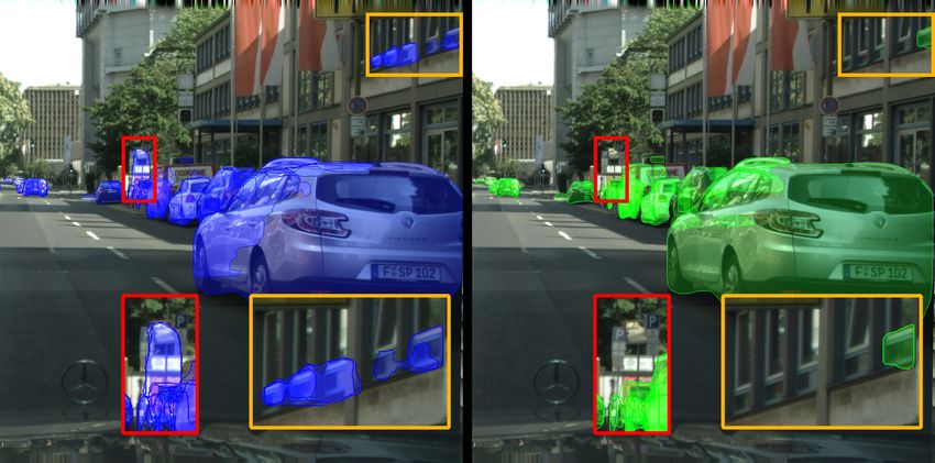
this range. Fig. 7 shows an example of the segmentation error ral Information Processing, L. Cheng, A. C. S. Leung,
being reduced after finetuning. and S. Ozawa, Eds. 2018, Lecture Notes in Computer
Science, pp. 96–106, Springer International Publishing.
[9] Y.-H. Lam, A. Zare, F. Cricri, J. Lainema, and M. M.
5. CONCLUSIONS Hannuksela, “Efficient adaptation of neural network fil-
ter for video compression,” in Proceedings of the 28th
The proposed content-adaptive finetuning technique can sig- ACM International Conference on Multimedia. 2020,
nificantly improve the coding performance especially for low MM ’20, pp. 358–366, Association for Computing Ma-
targeted bitrates. This technique does not require a differen- chinery.
tiable encoder and it is not dependent on the availability of
[10] Y. Hong Lam, A. Zare, C. Aytekin, F. Cricri, J. Lainema,
the task network or task ground-truth, therefore it can be eas-
E. Aksu, and M. Hannuksela, “Compressing weight-
ily adopted into most computer vision workflows that employ
updates for image artifacts removal neural networks,” in
3 Determined by the minimum and maximum achievable bitrates using our IEEE/CVF Conference on Computer Vision and Pattern
trained models: [0.034, 0.148] Recognition Workshops, 2019.Input Before: 0.026 BPP – 0.281 mAP Before: 0.131 BPP – 0.297 mAP
After: ↓ 4.332% – ↑ 6.979% After: ↑ 1.6×10⁻⁴ % – 0%
Input Before: 0.043 BPP – 0.294 mAP Before: 0.123 BPP – 0.358 mAP
After: ↓ 3.716% – ↑ 2.609% After: ↓ 2.3×10⁻³ % – 0%
Fig. 6. Finetuning effects on different targeted bitrates. In each row, the leftmost image is the uncompressed input and the other
images are the `1 -norm difference images between the baseline outputs and the finetuned ones for different targeted bitrates.
The gains after finetuning are given under the images. The finetuning process modifies the areas around the edges and surfaces
of the objects in low-bitrate targeted output, which allows for higher coding gains.
R-CNN,” in 2017 IEEE International Conference on
Computer Vision (ICCV), 2017, pp. 2980–2988.
[15] S. Liu and W. Deng, “Very deep convolutional neural
network based image classification using small training
sample size,” in 2015 3rd IAPR Asian Conference on
Pattern Recognition (ACPR), 2015, pp. 730–734.
[16] O. Russakovsky, J. Deng, H. Su, J. Krause, S. Satheesh,
S. Ma, Z. Huang, A. Karpathy, A. Khosla, M. Bernstein,
A. C. Berg, and L. Fei-Fei, “ImageNet large scale visual
recognition challenge,” International Journal of Com-
puter Vision (IJCV), vol. 115, no. 3, pp. 211–252, 2015.
[17] M. Cordts, M. Omran, S. Ramos, T. Rehfeld, M. En-
Fig. 7. Error reduction of segmentation before and after the zweiler, R. Benenson, U. Franke, S. Roth, and
finetuning. Left: baseline results, right: finetuned results. B. Schiele, “The cityscapes dataset for semantic ur-
ban scene understanding,” in 2016 IEEE Conference
on Computer Vision and Pattern Recognition (CVPR).
[11] N. Zou, H. Zhang, F. Cricri, H. R. Tavakoli, J. Lainema, 2016, pp. 3213–3223, IEEE.
M. Hannuksela, E. Aksu, and E. Rahtu, “L2 C – learning [18] F. Brossen, J. Boyce, K. Suehring, X. Li, and V. Seregin,
to learn to compress,” IEEE 22nd International Work- “JVET common test conditions and software reference
shop on Multimedia Signal Processing, 2020. configurations for sdr video,” Joint Video Experts Team
[12] J. Campos, S. Meierhans, A. Djelouah, and C. Schroers, (JVET), Document: JVET-N1010, March 2019.
“Content adaptive optimization for neural image com- [19] D. P. Kingma and J. Ba, “Adam: A method for stochastic
pression,” in IEEE/CVF Conference on Computer Vi- optimization,” in International Conference on Learning
sion and Pattern Recognition Workshops, 2019. Representations (ICLR) 2015.
[13] H. Zhang, F. Cricri, H. R. Tavakoli, N. Zou, E. Aksu, [20] G. Bjontegaard, “Calculation of average psnr differ-
and M. M. Hannuksela, “Lossless image compression ences between RD-curves,” ITU-T Video Coding Ex-
using a multi-scale progressive statistical model,” in perts Group (VCEG), 2001.
Proceedings of the Asian Conference on Computer Vi-
sion (ACCV), November 2020.
[14] K. He, G. Gkioxari, P. Dollár, and R. Girshick, “MaskYou can also read