Irreversibility and biased ensembles in active matter: Insights from stochastic thermodynamics - arXiv
←
→
Page content transcription
If your browser does not render page correctly, please read the page content below
Irreversibility and biased
                                                 ensembles in active matter:
                                                 Insights from stochastic
                                                 thermodynamics
arXiv:2104.06634v1 [cond-mat.soft] 14 Apr 2021

                                                 Étienne Fodor,1 Robert L. Jack,2,3
                                                 and Michael E. Cates2
                                                 1
                                                   Department of Physics and Materials Science, University of Luxembourg,
                                                 L-1511 Luxembourg; email: etienne.fodor@uni.lu
                                                 2
                                                   Department of Applied Mathematics and Theoretical Physics, University of
                                                 Cambridge, Wilberforce Road, Cambridge CB3 0WA, United Kingdom; email:
                                                 rlj22@cam.ac.uk, m.e.cates@damtp.cam.ac.uk
                                                 3
                                                   Yusuf Hamied Department of Chemistry, University of Cambridge, Lensfield
                                                 Road, Cambridge CB2 1EW, United Kingdom

                                                 Keywords
                                                 self-propelled particles, nonequilibrium field theories, dissipation,
                                                 entropy production, large deviations, phase transitions

                                                 Abstract

                                                 Active systems evade the rules of equilibrium thermodynamics by con-
                                                 stantly dissipating energy at the level of their microscopic components.
                                                 This energy flux stems from the conversion of a fuel, present in the
                                                 environment, into sustained individual motion. It can lead to collective
                                                 effects without any equilibrium equivalent, such as a phase separation
                                                 for purely repulsive particles, or a collective motion (flocking) for align-
                                                 ing particles. Some of these effects can be rationalized by using equi-
                                                 librium tools to recapitulate nonequilibrium transitions. An important
                                                 challenge is then to delineate systematically to which extent the char-
                                                 acter of these active transitions is genuinely distinct from equilibrium
                                                 analogs. We review recent works that use stochastic thermodynamics
                                                 tools to identify, for active systems, a measure of irreversibility com-
                                                 prising a coarse-grained or informatic entropy production. We describe
                                                 how this relates to the underlying energy dissipation or thermodynamic
                                                 entropy production, and how it is influenced by collective behavior.
                                                 Then, we review the possibility to construct thermodynamic ensembles
                                                 out-of-equilibrium, where trajectories are biased towards atypical val-
                                                 ues of nonequilibrium observables. We show that this is a generic route
                                                 to discovering unexpected phase transitions in active matter systems,
                                                 which can also inform their design.

                                                                                                                    1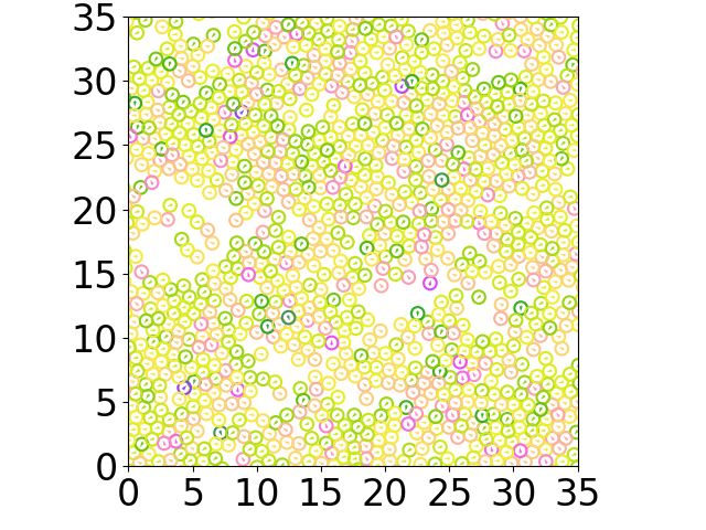
1. INTRODUCTION
    Active matter is a class of nonequilibrium systems whose components extract energy from
    the environment to produce an autonomous motion (1, 2, 3). Examples are found in biolog-
    ical systems, such as swarms of bacteria (4) and assemblies of cells (5); social systems, such
    as groups of animals (6) and human crowds (7); synthetic systems, such as vibrated polar
    particles (8) and self-catalytic colloids (9). The combination of individual self-propulsion
    and interactions between individuals can lead to collective effects without any equivalent
    in equilibrium. Examples include collective directed motion, as observed in bird flocks (6),
    and the spontaneous formation of clusters made of purely repulsive particles, as reported for
    Janus colloids in a fuel bath (9). To study these effects, minimal models have been proposed
    based on simple dynamical rules. Some are formulated at the level of individual particles,
    for instance with automaton rules (10) or by extending Langevin dynamics (11). Others
    describe the system at coarse-grained level in terms of hydrodynamic fields (12, 13). The
    latter can be obtained systematically by coarse-graining the particle dynamics or postulated
    phenomenologically. Both the microscopic and hydrodynamic approaches have successfully
    reproduced experimental behavior, such as the emergence of a long-ranged polar order,
    known as the flocking transition (14), and phase separation that occurs without any micro-
    scopic attraction, known as motility-induced phase separation (MIPS) (15).
        Although active systems evade the rules of equilibrium statistical mechanics, some works
    have built a framework to predict their properties based on the partial applicability of
    thermodynamic concepts beyond equilibrium. A first approach was to map some active
    systems onto equilibrium ones with a similar steady state, allowing one to define effective
    free-energies for active matter (16, 17). Other studies have extended the definitions of
    standard observables including pressure (18, 19, 20), surface tension (21, 22), and chemical
    potential (23, 24), hoping to establish equations of state relating, for instance, pressure and
    density. Interestingly, one finds that the existence of such state functions cannot generically
    be relied upon (e.g., the pressure on a wall can depend on the type of wall) (20), highlighting
    the limitations of equilibrium analogies. In trying to build a thermodynamic framework
    for active matter, an important challenge is then to identify regimes where it is possible
    to deploy equilibrium tools, and to clearly distinguish these from genuine nonequilibrium
    regimes. In other words, how should we delineate where and when activity really matters
    in the emerging phenomenology? And, most importantly, can we define a systematic,
    unambiguous measure of the departure from equilibrium?
        In passive systems, the steady state (Boltzmann) distribution involves the Hamilto-
    nian which also drives the micro-dynamics. This ensures thermodynamic consistency of
    the dynamics, which further implies that the mechanical and thermodynamic definitions
    of pressure are equivalent, and precludes (real space) steady-state currents. While such
    currents offer a clear nonequilibrium signature of activity, as observed for instance in col-
    lective motion (14), it is more challenging to distinguish, say, MIPS from standard phase
    separation without tracking individual particle motion (15). In particular it is not helpful
    to define departure from equilibrium via deviation from an effective “Boltzmann distri-
    bution” in systems that are not thermodynamically consistent. Instead, the cornerstone
    of modern statistical mechanics, which allows one to dissociate fundamentally active and
    passive systems, is the reversibility of equilibrium dynamics (25). In a steady equilibrium
    state, forward and backward dynamics are indistinguishable, since all fluctuations exhibit
    time-reversal symmetry (TRS). This constraint entails other important properties, such as
    the fluctuation-dissipation theorem (FDT) (26), and the absence of dissipated heat at equi-

2   Fodor • Jack • Cates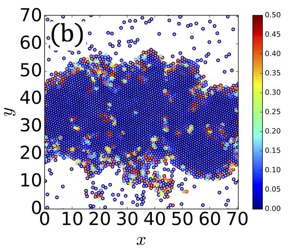
librium. For active systems, the irreversibility of the dynamics then stands out as the key
differentiating property that causes the violation of these and other equilibrium laws.
    To quantify the breakdown of TRS, we use stochastic thermodynamics (27, 28). This
framework extends standard notions of thermodynamics, such as the first and second laws,
to fluctuating trajectories. It was first developed for systems in contact with one or more
reservoirs, such as energy and/or volume reservoirs, provided that each reservoir satisfies
some equilibrium constraints. Such constraints do not preclude the system to operate out-of-
equilibrium, for instance under external fields and/or thermostats at different temperatures:
In this context, the thermodynamic consistency of the dynamics yields some explicit con-
nections between irreversibility, dissipated heat and entropy production. In contrast, the
dynamics of active systems are often formulated via phenomenological arguments, which do
not follow a priori the requirements of thermodynamic consistency. A natural question is
then: Is it legitimate to extend the methods of stochastic thermodynamics to active matter?
And, what can we learn from its irreversibility measures when their connection with other
thermodynamic observables becomes blurred?
    Another interesting direction in active matter theory is to generalize familiar thermo-
dynamic ensembles to nonequilibrium settings. Here the important role of steady-state
currents and other types of irreversible dynamics make it insufficient to study ensembles of
configurations (characterized by a stationary measure, of which the Boltzmann distribution
is an example). Instead we must address ensembles of trajectories, as used previously to
analyze fluctuation theorems (29), and other dynamical effects (30, 31, 32). Such ensem-
bles are built similarly to the canonical ensemble of statistical mechanics, with relevant
(extensive) observables coupled to conjugate (intensive) fields. In practice, one selects a
dynamical observable of interest and focusses on dynamical trajectories where it has some
atypical target value. The resulting biased ensembles of rare trajectories, are intrinsically
connected to large deviation theory (33, 34). As such, they provide insight into mechanisms
for unusual and interesting fluctuations. In the passive context, they have proven useful
for unveiling dynamical transitions, e.g., in kinetically constrained models of glasses (32).
This leads one to ask: How do the transitions in biased ensembles of active matter differ
from their passive counterparts? And then, can we identify settings in which bias-induced
transitions emerge in active matter that have no passive equivalent?
    In what follows (Section 2), we describe how the irreversibility of active systems can be
quantified, both for particle-based and hydrodynamic theories, using generalized forms of
entropy production. We discuss how to relate these, in certain cases, to energy dissipation,
and how they allow to identify phases and/or spatial regions where activity comes to the fore.
In Section 3, we then describe how biased ensembles provide novel insights on the emergence
of collective effects in active matter. We review some useful tools of large deviation theory,
such as representing dynamical bias in terms of control forces, show the utility of these
methods in an active context, and discuss how they can reveal unexpected transitions in
generic active systems. In Section 4 we give a brief conclusion that includes implications of
these methods for the rational design of new materials.

2. IRREVERSIBILITY AND DISSIPATION
2.1. Modeling active matter: From particles to hydrodynamic fields
A typical particle-based dynamics starts from the seminal Langevin equation. Provided
that inertia is negligible, this balances the forces stemming from the heat bath (damping

                                                     Stochastic thermodynamics of active matter   3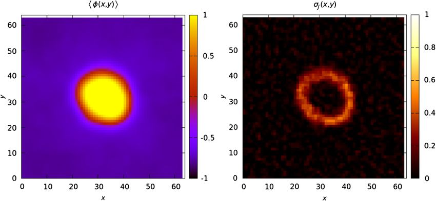
and thermal noise), the force deriving from a potential U , and non-conservative forces fi :
                                                               p
                                      ṙi = µ fi − ∇i U ) +     2µT ξi ,                             1.

    where µ is the mobility, T the temperature of the bath, and ξi a set of zero-mean, unit-
    variance white Gaussian noises: hξiα (t)ξjβ (t0 )i = δij δαβ δ(t − t0 ), where Latin and Greek
    indices respectively refer to particle labels and spatial coordinates. Hereafter, we refer to
    such noise as unit white noise. The potential U describes particle interactions and/or an
    external perturbation applied by the operator. The non-conservative forces fi model self-
    propulsion, which converts a source of energy, present in the environment, into directed
    motion. In principle, fi can include external perturbations that do not derive from a po-
    tential. When fi = 0, the system is at equilibrium with Boltzmann statistics (∝ e−U/T ).
        The self-propulsion force fi is often modeled as effectively an additional noise. In con-
    trast with the thermal noise ξi , it has some persistence which captures the propensity of
    active particles to sustain directed motion. Typically, a persistence time τ sets the exponen-
    tial decay of the two-point correlations: hfiα (t)fjβ (0)i = δij δαβ f02 e−|t|/τ . In recent years,
    two variants have emerged as popular models of self-propelled particles. First, for Active
    Ornstein-Uhlenbeck Particles (AOUPs), the statistics of fi is Gaussian, so that it can be
    viewed as obeying an (autonomous) Ornstein-Uhlenbeck process (17, 35):
                                                                 √
                                     AOUP :      τ ḟi = −fi + f0 2τ ζi ,                            2.
                                                                            p
    where the ζi are unit white noises. Scaling the amplitude as µf0 =        µTa /τ , the self-
    propulsion itself converges to a white noise source in the limit of vanishing persistence,
    in which regime the system reduces to passive particles at temperature T + Ta . Second,
    for Active Brownian Particles (ABPs), the magnitude of fi is now fixed, which leads to
    non-Gaussian statistics, described by the following process in two dimensions (11):
                                                                            p
                             ABP :    fi = f0 (cos θi , sin θi ),   θ̇i =    2/τ ηi ,                3.

    where ηi is a unit white noise. In Equations 2 and 3, the self-propulsion is independent for
    each particle. This corresponds to isotropic particles, which undergo MIPS for sufficiently
    large persistence and density (15). In contrast, many models consider alignment interac-
    tions, yielding a collective (oriented) motion at high density and enhanced persistence (14).
        To study the emergence of nonequilibrium collective effects, it is helpful to introduce the
    relevant hydrodynamic fields. These can be identified, and their dynamical equations found,
    by coarse-graining the microscopic equations of motion, using standard tools of stochastic
    calculus (36). Another approach consists in postulating such hydrodynamic theories from
    phenomenological arguments, respecting any conservation laws and spontaneously broken
    symmetries (1). For instance, a theory of MIPS can be found by considering the dynamics
    of a scalar field φ(r, t) that encodes the local concentration of particles (13, 37):

                                                                  √

                                                         δF
                           φ̇ = −∇ · J = −∇ ·       − λ∇    + Jφ + 2λDΛφ ,                           4.
                                                         δφ

    where λ is collective mobility, D a noise temperature, and Λφ (spatiotemporal) unit white
    noise. The term Jφ embodies contributions driving the current J of φ that cannot be
    derived from any “free energy” functional F as −λ∇(δF/δφ). For instance, choosing a
    standard φ4 , square-gradient functional for F captures phase separation in equilibrium. On

4   Fodor • Jack • Cates
introducing activity, symmetry arguments enforce that Jφ takes the form ∇(∇φ)2 and/or
(∇φ)(∇2 φ) to lowest order in φ and its gradients (13, 37). The former term shifts the
coexisting densities with respect to the equilibrium model (13), whereas the latter can lead
to microphase separation, with either the vapour phase decorated with liquid droplets, or the
liquid phase decorated with vapour bubbles (37). Note that, although the conservative term
−λ∇(δF/δφ) captures all the contributions to the coarse-grained dynamics that respect
TRS, it may be depend on nonequilibrium parameters of the microscopic dynamics (37).
The dynamics in Equation 4 can also be coupled to a polar field p(r, t), representing
the local mean orientation of particles, to study for instance collective flocking motion (14):
δF √
ṗ = − + Jp + 2DΛp , 5.
δp
where the rotational mobility is taken as unity, and Λp is another spatiotemporal unit white
noise. As with Jφ , the term Jp represents active relaxations that cannot be written as free-
energy derivatives. Note that, for the passive limit of the coupled model to respect detailed
balance, the free energy F in Equation 5 must be the same as that in Equation 4, and the
value of D in each equation must also coincide. In the absence of activity (Jφ = Jp = 0),
the system has Boltzmann statistics ∝ e−F /D . To capture the emergence of polar order, a
minimal choice is to take F as a p4 functional, with Jφ proportional to p, and Jp a linear
combination of ∇φ, φp and (p · ∇)p (1, 14). This can yield polar bands traveling across an
apolar background, which is a key signature of aligning active particles models (10). In fact,
much of the physics of flocks is retained by setting λ = 0 in Equation 4 (12). On the other
hand, more complicated theories, describing the emergence of nematic order (14) and/or
the coupling to a momentum conserving fluid (38, 39), introduce additional hydrodynamic
fields beyond φ and p as considered above.
2.2. How far from equilibrium is active matter?
2.2.1. Forward and time-reversed dynamics: Path-probability representation. To quan-
tify the irreversibility of active dynamics, we compare the path probability P to realize
a dynamical trajectory (across a time interval [0, t]) with that for its time-reversed coun-
terpart (27, 28, 40). As we shall see, choosing the time-reversed dynamics is a matter of
subtlety (35, 39, 41, 42, 43, 44, 45, 46, 47, 48, 49). For the particle-based dynamics in Equa-
tion 1, exploiting the known statistics of the (unit white) noise, trajectories of position ri
and self-propulsion fi have probability P ∼ e−A (50), with action
Z t Xh
1 i2
A= ṙi + µ ∇i U − fi dt0 + Af . 6.
4µT 0 i
We use Stratonovitch discretization, omitting a time-symmetric contribution that is irrele-
vant in what follows. Af specifies the statistics of the self-propulsion force fi . For AOUPs
and ABPs, fi has autonomous dynamics, independent of position ri . One can then in
principle integrate out that dynamics to obtain a reduced action Ar . So far, the explicit
expression has been derived only for AOUPs (35, 48, 51, 52):
Z t Z t X
dt0 dt00 ṙi + µ∇i U t0 · ṙi + µ∇i U t00 Γ(t0 − t00 ).
Ar = 7.
0 0 i
The kernel Γ is an even function of time t, which depends on µ, T , f0 , and τ . It reduces
to Γ(t) = δ(t)/(4µ(T + Ta )) for vanishing persistence (τ = 0), when the self-propulsion
Stochastic thermodynamics of active matter 5p
amplitude scales as µf0 = µTa /τ (48), as expected for passive particles. The actions
A and Ar describe the same dynamics from different viewpoints. The former tracks the
realizations of position and self-propulsion, whereas the latter follows the time evolution of
positions only. Thus Ar treats the self-propulsion as a source of noise, without resolving
its time evolution. In contrast, A regards fi as a configurational coordinate, which might
in principle be read out from the particle shape. For instance, Janus particles, which are
spheres with distinct surface chemistry on two hemispheres (2, 9), generally self-propel
along a body-fixed heading vector pointing from one to the other. See also Figure 1.
To compare forward and backward trajectories, one needs to define a time-reversed
version of the dynamics. This necessarily transforms the time variable as t0 → t − t0 , and it
can also involve flipping some of the variables/fields (as detailed below). For particle-based
dynamics, time reversal of the positions ri is unambiguous. Writing P in terms of the
reduced action Ar in Equation 7, the time-reversed counterpart AR r reads
Z t Z t X
AR dt0 dt00 Γ(t0 − t00 ) .
r = ṙi − µ∇i U t0
· ṙi − µ∇i U t00
8.
0 0 i
Here we have changed variables as {t0 , t00 } → {t−t0 , t−t00 }, and used that Γ is even. For the
full action A, defining the time-reversed dynamics requires that we fix the time signature
of the self-propulsion fi . Indeed, there are two possible reversed actions, AR,± , where +
and − indices refer respectively to even (fi → fi ) and odd (fi → −fi ) self-propulsion:
Z t
1 Xh i2
AR,± = ṙi − µ ∇i U ∓ fi dt0 + Af . 9.
4µT 0 i
We assumed that Af is the same for forward and time-reversed dynamics which holds
for ABPs/AOUPs (but not for systems with aligning interactions (53)). AR r and A
R,±
correspond to three different definitional choices of the time-reversed dynamics. The first of
these deliberately discards the realizations of the self-propulsion forces, in order to compare
the forward and backward motion of particle positions. This choice is widely used for
AOUPs, where particles have no heading vector. It is also the only possible choice when
T = 0 in Equation 1, see (35). In contrast, AR,± , which each assume that both position and
self-propulsion are tracked, are usually chosen for particles with a heading vector (54, 45, 53).
For the field theories of Section 2.1, defining the time-reversed dynamics requires us to
choose the time signature of each field. This choice depends on the physical system and the
phases under scrutiny (Section 2.4). Scalar fields associated with a local density are clearly
even (13, 39), whereas scalar fields schematically representing polarization (55), or stream
functions for fluid flow (56), should generally be odd. Similarly, the vector field p can be
chosen even (57) or odd (47), depending on whether it is viewed as the local orientation of
particles (mean heading vector, see Figure 1) or directly as a local velocity (12). One also
has to decide which fields to retain or ignore when comparing forward and backward paths.
This choice is the counterpart at field level of retaining (A) or ignoring (Ar ) the propulsive
forces in a system of AOUPs. For example, in a system with φ and p variables, one can
choose whether or not to keep separate track of the density current J alongside φ and p.
In general, there are four different versions for time-reversed dynamics of Equations 4
and 5, provided that each one of the fields φ and p can be either odd or even. Often,
though, constraints on the time signatures of the fields restrict these choices. To ensure
that the dynamics is invariant under time reversal in the passive limit, the free energy F
6 Fodor • Jack • Catesorientation reversal
(a) (b)
time reversal
(c) (d)
Figure 1
Time reversal (TR) for active particles (fish). Each has an orientation (head-tail axis) and moves
(swims) as indicated by the wake lines behind it. The TR operation may or may not reverse
orientations. (a) Natural dynamics. (b) Reversing orientation but not motion: fish swim tail-first
along their original directions. (c) Reversing motion but not orientation: fish swim tail-first,
opposite to their original direction. (d) Reversing both motion and orientation: fish swim
head-first, opposite to their original direction. The situations in (b,c) occur with extremely low
probability in the natural dynamics (requiring exceptional noise realizations). In dilute regimes
(not shown) case (d) is equiprobable to (a): individual fish swim head-first in both cases. For the
shoals shown here, however, (d) is less probable than (a), because the natural dynamics has more
fish at the front of the shoal: TRS is broken at a collective level even if orientations are reversed.
must be the same in forward and time-reversed dynamics. This enforces that odd fields
can only appear as even powers in F. Hence if p appears linearly in F, which for liquid
crystal models often includes a p · ∇φ or anchoring term, it must be chosen even. Further
constraints arise if some of the possible noise terms are set to zero (e.g., (12)) so that certain
fields are deterministically enslaved to others. For instance if φ̇ = −∇ · p (without noise),
for consistency φ and p necessarily have different signatures.
2.2.2. Distance from equilibrium: Breakdown of time-reversal symmetry. For a given dy-
namics, once its time-reversed counterpart has been chosen, we can define systematically
an irreversibility measure S as (27, 28, 40)
1 P 1 R
S = lim ln R = lim A −A . 10.
t→∞ t P t→∞ t
The average h·i is taken over noise realizations. The limit of long trajectories gets rid of
any transient relaxations to focus on steady-state fluctuations. Equation 10 is a cornerstone
of stochastic thermodynamics (27, 28, 40). It was first established in thermodynamically
consistent models (40), where S can be shown to be the entropy production rate (EPR) gov-
erning the dissipated heat (27, 28). In models where S has this meaning, thermodynamics
constrains the choice of time reversal. In Section 2.3, we return to the question of how far
the thermodynamic interpretation extends to active systems. Meanwhile, S already offers
an unambiguous measure of TRS breakdown in active matter, which we refer to as infor-
Stochastic thermodynamics of active matter 7matic EPR (IEPR). Since S changes when the dynamics is coarse-grained, by eliminating
unwanted variables, it differs when retaining (A) or ignoring (Ar ) the propulsive forces.
In particle-based dynamics, choosing the action Ar so that only particle positions are
tracked, the corresponding IEPR Sr follows from Equations 7, 8 and 10 as
Z ∞ X
Sr = −4µ Γ(t) ṙi (t) · ∇i U (0) dt, 11.
−∞ i
where we have again used that Γ is even. The IEPR Sr vanishes in the absence of any
potential, showing that the dynamics satisfies TRS for free active particles, and also for an
external harmonic potential U ∼ r2i (35, 52). When T = 0, it reduces to Sr = τ h( i ṙi ·
P
∇i )3 U i/(2(µf0 )2 ) (35). When (by using the full action A) one follows the dynamics of both
position and self-propulsion, the two possible IEPRs found from Equations 6, 9 and 10, are
1 X µX
S+ = ṙi · fi , S− = ∇i U · fi . 12.
T i T i
RtP
We have used that 1t 0 i ṙi · ∇i U dt0 = U (t)−U t
(0)
vanishes at large t. Substituting in
Equation 12 the expression for ṙi from Equation 1 yields S + +S − = N µf02 /T , where N is the
√
particle number, using that self-propulsion fi and thermal noise 2µT ξi are uncorrelated.
Therefore, in the absence of any potential U , S − vanishes identically whereas S + remains
non-zero. Indeed, S − compares trajectories whose velocity and self-propulsion both flip on
time reversal, retaining alignment (up to thermal noise) between the two: The forward and
backward dynamics are indistinguishable unless potential forces intervene. In contrast, S +
quantifies how different trajectories are when particles move either along with, or opposite
to, their self-propulsion (Figure 1), yielding the contribution N µf02 /T even when U = 0.
The IEPR S + is lowest (and S − highest) when the propulsive force fi balances the
interaction force −∇i U so that particles are almost arrested. Hence, both IEPRs are sensi-
tive to the formation of particle clusters, which is associated with dynamical slowing-down
for isotropic particles (15), and to formation of a polarized state for aligning particles (14).
Note that S + is proportional to the contribution of self-propulsion to pressure, known as
swim pressure (19, 20). Finally, in the presence of alignment, any dynamical interaction
torques appear explicitly in S (53). We defer further discussion on how interactions shape
irreversibility, for both particle-based dynamics and field theories, to Section 2.4.
2.3. Energetics far from equilibrium: Extracted work and dissipated heat
2.3.1. Particle-based approach: Energy transfers in microscopic dynamics. A major suc-
cess of stochastic thermodynamics is to extend the definition of observables from classical
thermodynamics to cases where fluctuations cannot be neglected (27, 28, 40). Although
first proposed for thermodynamically consistent models, this approach can be extended to
some (not all) types of active matter. Considering that the potential U depends on the set
of control parameters αn , the work W produced by varying αn during a time t reads (27, 28)
Z t X ∂U 0
W= α̇n dt . 13.
0 n
∂αn
Note that W is stochastic due to the thermal noise and the self-propulsion, even though
the protocol αn (t) is deterministic. Equation 13 relies on the precept that some external
8 Fodor • Jack • Catesoperator perturbs the system though U , without prior knowledge of the detailed dynamics;
it applies equally for active and passive systems.
The heat Q is now defined as the energy delivered by the system to the surrounding
thermostat. For the dynamics of Equation 1, the effect of the thermostat is encoded in the
damping force and the thermal noise; the fluctuating observable Q then follows as (27, 28)
Z t X ṙi
· ṙi − 2µT ξi dt0 .
p
Q= 14.
0 i
µ
P
Substituting Equation 1 into Equation 14, and using the chain rule U̇ = n α̇n (∂U/∂αn ) +
P
i ṙi · ∇i U , gives a relation between energy U , work W, and heat Q:
Z t X
U (t) − U (0) = W − Q + ṙi · fi dt0 . 15.
0 i
In passive systems, the non-conservative force fi represents some intervention by the external
RtP
operator (beyond changes in U ), so that the term W̄ ≡ 0 i ṙi · fi dt0 can be absorbed
into the work W. Then, Equation 15 is the first law of thermodynamics (FLT) (27, 28).
The only possible time reversal for passive dynamics is to choose S + in Equation 12, so
that S + = Q̇/T . In this context, S + coincides with the thermodynamic EPR due to
contact of the system with the thermostat, which connects explicitly irreversibility, entropy
production, and dissipation (28). In contrast, for active dynamics, the contribution W̄
captures the energy cost to sustain the self-propulsion of particles (58, 59), which is generally
distinct from both W and Q. When the potential is static (α̇n = 0), S + = Q̇/T still holds,
yet S + should not be interpreted as a thermodynamic EPR in general.
Although these considerations offer one consistent approach to the question of energy
transfers for active particles, several other approaches are possible. Interestingly, one al-
ternative definition of heat relies on replacing ṙi in Equation 14 by ṙi − µfi . This amounts
to regarding the self-propulsion as caused by a locally imposed flow, with particle displace-
ments evaluated in the flow frame (48, 43). It yields vanishing heat in the absence of
interactions, for the same reasons as led us to zero S − in Equation 12. Also, some works
√
addressing heat engines (60, 61, 62) have redefined heat by replacing 2µT ξi in Equation 14
√
with 2µT ξi + µfi , thus considering the self-propulsion fi as a noise with similar status to
√
2µT ξi . This yields vanishing heat when the potential is static (α̇n = 0), by discarding all
the energy dissipated by self-propulsion, allowing one to reinstate FLT, U (t)−U (0) = W−Q.
Finally, the angular diffusion of ABPs is often itself regarded
p as thermal. This gives an
RtP
angular contribution to Q, proportional to 0 i θ̇i (θ̇i − 2/τ ηi )dt0 , which vanishes for
Equation 3, but is generally non-zero when aligning interactions are present (59). For
AOUPs, interpreting the self-propulsion dynamics in terms of thermal damping and noise
is less straightforward, although some studies have taken such a path (41, 42, 63).
Importantly, Equation 1 does not resolve how particles convert fuel into motion. Ac-
cordingly, Equation 14 only captures the energy dissipated by the propulsion itself, ignoring
contributions from underlying, metabolic degrees of freedom. Various schematic models de-
scribe the underlying chemical reactions in thermodynamically consistent terms, maintain-
ing them out-of-equilibrium by holding constant the chemical potential difference between
products and reactants (43, 46, 64). For some of these models (43, 46), the time evolution
of ri can be mapped into Equation 1 when a chemical noise parameter is small (58). In this
case, the difference between the partial and total heat, found by discarding or including
Stochastic thermodynamics of active matter 9reactions, is a constant, independent of the potential U . In a more refined model, the dy-
namics tracks the time evolution of chemical concentration, and the heat features explicitly
the chemical current (64). Related features will emerge next, for continuum fields.
2.3.2. Coarse-grained perspective: Energy transfers at hydrodynamic level. For field the-
ories, assuming that the free energy F depends on some set of control parameters αn , the
work W is defined by analogy with Equation 13 as
Z tX
∂F 0
W= α̇n dt . 16.
0 n
∂α n
This holds regardless of any additional nonequilibrium terms in Equations 4 and 5, and
can be viewed as directly generalizing from the case of passive to active fields. In con-
trast, to define heat at a hydrodynamic level, one cannot depend a priori on a physical
interpretation of the various dynamical terms as we made for particles. A minimal require-
ment, for emergence of FLT along the lines of Equation 15, is that F in Equation 16 is
a genuine free energy, which stems from coarse-graining only the passive contributions of
the microscopic dynamics. When theories are based solely on phenomenological arguments,
this thermodynamic interpretation is absent.
In some cases, nonetheless, an active field theory ought to allow a thermodynamic in-
terpretation, e.g. for the formation of membraneless organelles (65). In contrast, we do not
expect this if the same theory is used to describe the demixing of animal groups. To reinstate
a thermodynamic framework, one can include chemical fields describing the fuel consump-
tion underlying activity (57). This approach relies on linear irreversible thermodynamics
(LIT) (66), as previously used to illuminate particle-based dynamics (64). LIT postulates
linear relations between thermodynamic fluxes and forces, whose product determines the
heat Q. A class of active gel models were indeed first formulated in this way (67, 68). In
contrast, the field theories in Equations 4 and 5 were not derived from LIT a priori, yet
they can be embedded within it in a consistent manner.
To illustrate this, consider a scalar field φ obeying Equation 4. The conservation law
φ̇ = −∇ · J relates this to the thermodynamic flux J, whose conjugate force is −∇(δF/δφ).
Likewise a thermodynamic flux ṅ describes some metabolic chemical process, with conjugate
force a chemical potential difference ∆µ. Out-of-equilibrium dynamics is maintained by
holding either ṅ or ∆µ constant (47). Considering here the latter case, LIT requires that
the active current Jφ is linear in ∆µ (although, like J, it can be nonlinear in φ), so that we
identify Jφ /∆µ ≡ C as an off-diagonal Onsager coefficient (57), yielding
δF
J, ṅ = L − ∇ , ∆µ + noise terms, 17.
δφ
with Onsager matrix obeying LJJ = λI (with I the d-dimensional identity); Lṅṅ = γ, a
chemical mobility (such that ṅ = γ∆µ in the absence of φ dynamics); and LJṅ = LṅJ = C.
This last result encodes the famous Onsager symmetry which stems from the underlying
reversibility of LIT (25), so that the form of the active current Jφ also controls the φ coupling
in the equation for ṅ. For Jφ = ∆µ∇((∇φ)2 ) (13), then ṅ = γ∆µ − ∇(δF/δφ) · ∇((∇φ)2 ).
The covariance of the noise terms in Equation 17 is set directly by L. The off-diagonal
noise depends on φ through C and thus is multiplicative. The noise terms accordingly
include so-called spurious drift contributions, which ensure that the LIT dynamics reaches
Boltzmann equilibrium when neither ṅ nor ∆µ is held constant (57).
10 Fodor • Jack • CatesA crucial assumption of Equation 17 is that φ and n are the only relevant hydrody-
namic fields, so that, on the time and length scales at which they evolve, all other degrees
of freedom are thermally equilibrated. Then, the heat Q is given in terms of the entropy
production of these fields: Q = D ln(P[J, ṅ]/P R [J, ṅ]). The resulting thermodynamic EPR
differs in form from the informatic EPR associated with the dynamics of φ alone (Equa-
tion 10). Therefore, it cannot be equated with any of the various IEPRs for differently
time-reversed pure φ dynamics given in Section 2.2. On the other hand, since Equation 17
follows LIT, the heat can be expressed in terms of currents and forces:
Z Z t
0 δF
Q = dr dt J · ∇ + ṅ∆µ . 18.
0 δφ
Similar expressions arise for more elaborate field theories, such as polar fields (57). Note
that Q is stochastic, as is W in Equation 16, even though both are defined at hydrodynamic
P R
level. Using the chain rule Ḟ = n α̇n (∂F/∂αn ) + φ̇(δF/δφ)dr and the conservation law
φ̇ = −∇ · J, it follows that free energy F, work W, and heat Q are related as
Z Z t
F(t) − F (0) = W − Q + dr dt0 ṅ∆µ. 19.
0
The energy balance in Equation 19 offers the hydrodynamic equivalent of the relation be-
tween the particle-based work W, heat Q, and energy U in Equation 15. When neither ṅ
nor ∆µ is maintained constant, and ∆µ derives from a free energy (∆µ = −δFch /δn), the
system achieves equilibrium, so that Equation 19 reduces to FLT with respect to the total
free energy F + Fch . When the free-energy F does not change (α̇n = 0), the heat rate
R
equals dr hṅ∆µi, which illustrates that all the activity ultimately stems from the work
R
done by chemical processes. At fixed ∆µ (say), ṅ depends on φ, so that dr hṅ∆µi contains
information similar to, but distinct from, Equation 10, see discussion in Section 2.4.
2.4. Where and when activity matters
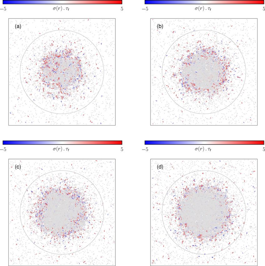
2.4.1. Spatial and spectral decompositions of irreversibility. The various IEPRs introduced
in Section 2 enable one to delineate regimes where activity most affects the dynamics com-
pared to equilibrium. Identifying such regimes can quantify the length and time scales where
activity primarily matters, and sometimes pinpoint specific locations where self-propulsion
plays an enhanced role. Within this perspective, the most appropriate choice of IEPR is
usually that which best reflects the dynamical symmetries of the emergent order (see Figure
1). By eliminating gross contributions (e.g., from propulsion pointing opposite to velocity)
the right choice of IEPR can help identify dynamical features which break TRS more subtly,
and help unravel how activity can create effects with no equilibrium counterpart.
If thermal noise is omitted from Equation 1, only one IEPR can be defined. This
is Sr (see Equation 11), tracking positions only. For AOUPs with pairwise interaction
P P
U = i1.6 35
(c)
1.4 (b) 30
1.2 25
ρ(r ) . a 2 10− 3
σ (r ) . a 2 τr
1.0 20
(a) 0.8 15
0.6 10
0.4 5
0.2 0
0.0
NTROPY PRODUCTION IN FIELD THEORIES WITHOUT … PHY S. REV. X 7, 021007 (2017)
0 10 20 30 40 50 60 70
r/ a
1 (c) 0.004
0.5 0.002
⟨φ(x)⟩
σφ (x)
0 0
⟨φ (x)⟩
-0.5 D = 0.001 -0.002
D = 0.002
D = 0.02
-1 D = 0.04 -0.004
FIG. 6. Snapshots of AOUPs interacting via the short-range soft-core potential (85), and 0
conf ned in a harmonic potential U (r) = U0 (r/ a0 )2
40 80 120 160 200 240
with f nite range a0 . The range of the potential is represented by the gray circle. The color of each particlexrefers to the associated instantaneous
value of the entropy production rate, expressed in units of 1/ τr = ε/ a2 . We observe that particles form a dense compact cluster centered at the
FIG. 6. Snapshots of AOUPs interacting via the short-range soft-core potential (85), and conf ned in a harmonic potential U (r) = U0 (r/ a0 )2
bottom of the harmonic trap with radial symmetry, in contact with a dilute bath of particles. The interface between the dense and dilute phases
. 1. Left with
panel: 2
Figure ffuctuates,
nite range
Density map athe
andof0 .afluctuatingphase-separated
The range
relative sizeof
of the
the potential
dense phaseisincreases
represented
droplet by
the the grayofcircle.
inActiveModel
with number B inThe
particles 2D.color
from of(d).
Center
(a) to each particle
panel: Local
Number refers to(a)
theN associated
contribution
of particles: 5625, instantaneous
= to
2
value(b)of
entropy production σð the
NrÞ entropy
=showing
6750, (c) Nproduction
a=strong rate,
N =expressed
contribution
7875, (d) at in
9000. Other theunits of 1/
interfaces.
parameters: L= = ε/Da=
τr 150,
Right . 1,
We U0observe
panel: 2, ε =that
=Density aparticles
10,and 1, τ =form
= entropy a0a=dense
60. compact
10,production for a 1D cluster centered at the
tem comSpatial decomposition
prisingbottom
a single dom
of the harmonic of
forthe
ain wall,trap with IEPR
various noise
radial (39,
symmetry,69).
levels in ≪(a) Phase
a22=
D contact 4a4. a
with Theseparation
entropy
dilute of repulsive
bath ofproduction
particles. is strongly
The active
interface inhom particles,
ogeneous,
between the dense and dilute phases
ning afinitevalueasD
with findividual
uctuates, →and
written as0at
σ itheinterfacebetween
the relative size of thevia
(color-coded denseanddiluteregionsandconvergingto
dense phase increases
Equation 20) with the
(q(tnumber
enhanced − s),atofthe
−p(t zero
particles inthebulk
from
can(a)
liquid-vapor
− s)), this be to inthislim
(d). Number
interface.
recast into it.of
Values
particles: (a) N = 5625,
(b)
he param eters used
Time-averaged are a
(b) N = 6750, ¼−0.125,
2 profiles a
(c) N = 7875, ¼0.125,
of4 particle κ ¼8,
(d) N = 9000. and
Other ρ
density λ ¼2.
parameters:
and IEPR L = 150,
density = 2, εthat
D = 1,σU0show = 10, σa= τ = 10,ina0 both
is1,small = 60.
bulks and peaked A(tZ) B(0)= D[q, p]Ps [q(0),
at the interface. (c)p(0)]δ( q̇ − p)behavior for a conserved active scalar field φ.
Similar
written
S ¼Sas discretized system A(t )(q(t − s), −p(t
exactly
B(0)= −
R s)),
, pR ]δ(this
respects −can bes [qrecast
q̇R detailed
pR )P R
balance
(t into
), −p R
(t )]
ϕ≡ σϕðrÞdr: ð19Þ D[q
× e−A [q,p] A(t ) B(0), (89)
whene ver λ ¼0, asR shown R
in Appendix B where further
R R
−A [q ,p ]+δA [q ,p ] R R R R
×e are given. For
inq̇ −
A(t
we)AhaveB(0)= p]P s [q(0), p(0)]δ( p) details A(q num
(0), perical
(0))B(q (t ), p (t )),
re and in Eq. (18), where added
is the a
D[q,subscript
dynamical action ϕdef toned num erical
(74). purposes, we
tinguishclusters,
these form which can
s fromvariable
Changing e potentially
xpressions appearing
from (q(s),
lead
p(s)) to laterto nonequilibrium
(qR (s), e
pvaluate
R
(s)) = the entropyA(t
(orproduction
motility-induced)
) B(0)= density D[qasR phase separa-
, pR ]δ(q̇R − pR )P (90) R R
s [q (t ), −p (t )]
−A [q,p]
ec. V) intion
which(15).
thecurrent
For Ja rather × e thedensity
than
phase-separated A(tdensity
)field
B(0), profile, (89)
Equation 20 Zallows one to distinguish the
1
s used to define trajectories. 032607-13
σϕ ðrÞ¼−lim μAðr;
−A [qR ,pR ]+δA [qRtÞ R 2
,p∇] μðr; tÞdt;pR (0))B(q ð21ÞR (t ), pR (t )),
relative contributions from particles in ×e A(qRphase,
(0),
where
As already mentioned A is theEq.
following dynamical
(9) above, action
thereare defdifferent
ned in (74). spatial zones.
t→∞ Dt In the dilute collisions
arelocal
eral other Changing
rare so thatvariable
quantitiesthat from small,
σhavethesam
i stays (q(s), p(s))
einte whereas
gral, S, (qR (s),
to in apRdense
whose (s)) = enough phase,
equivalencewith Eq. (18) is particles
established, barely
withinmove our so (90)
d hencethat
have equal
σi isclaim
again to be called the
modest. Atlocal entropy collisions
interfaces, discretization scheme, in
between Appendix
fast and slow D. particles, entering
duction density. Indeed, Our num 032607-13
erics in both one and two dimensions show
respectively from dilute and dense zones,that lead to locally high IEPR; see Figure 2.
the local entropy production density σϕðrÞis strongly
−σϕD ≡ hμϕi _
In; the hμAϕi_ ; hJ :∇μof Ai ;thermal
−hJ :J di noise, ð20Þ oneinhom ±
presence canogene alsoousstudysinceSit is(45).
large at These IEPRs
the interface track the
between
dynamics of both position and self-propulsion. phases but The sm all within these phases
corresponding (Fig. 1). To quantities,
particle-based quanti-
all equivalentfor thepurposesof computingS. Thefirst tatively explain this, weconsider theweak noiseexpansion
+ −
o formsσ differ
i = by(1/T
a transient
)hṙi contribution
· fi i and σ ΔFi =τ =→(µ/T 0, as )h∇ ofi Uthe· density
fi i, which take fi to be even and odd, are
thelast two. Thelatter pair arefoundfromtheformer by pffi ffi
ffiffihappens when −∇i U is equal
respectively minimal and maximal
tial integration, differingfromthemby termsof theform
for particles at rest. This
+ ϕ ¼ϕ0 þ Dϕ1 þ Dϕ2 þ OðD3=2Þ: ð22Þ
and opposite
ϒ d;A, where ϒ d ¼J μ and to ϒfiA. ¼J
In μpractice,
A . Our num σ erical
i is low in the dense phase and high at the interface (like
dies suggest that these alternative In theweak noiselim it, standard field-theoretical m ethods,
σi above), whereas σi candidates
−
decreases forgradually
local from the bulk of the dense phase to the interface.
whichweoutlineinAppendix E, show thatthedynamicsof
ropy production are practically indistinguishable in the
Considering instead polar clusters,
e of Active Model B. A more complex situation arises which ϕemerge
0 and ϕ1 when reducealigning
to interactions are present, σi−
Activeis Model
nowBþ low, as
indescribed
the dense in Sec.
andV.dilute phases, with a higher value _0 ¼−∇ at the interface (53). Thus, for
ϕ · J dðϕ0Þ; ð23Þ
isotropic particles it is σ + that exposes the character of the irreversibility of self-propulsion
A. Spatial decomposition of entropyi production
at interfaces, whereas for aligning particles σi− does so. Each separately elucidates the role
_1 ¼∇ 2 δF 0 þ 2λ∇ϕ0 · ∇ϕ1 þ ∇ · Γ;
We now turn to the numerical evaluation of σϕðrÞ in ϕ ð24Þ
of interfacial
tive Model B. We defer to self-propulsion to promote
futurework any study of the δϕ1
and stabilize clustering.
ical region of the model,
Turning focusing
now instead
to field on the weak
theories, we consider
whereΓfirst the simplest scalar model of Equation
isastandardGaussianwhitenoiseasinEq. (2) and 4,
se limit (small D) where sharp interfaces formbetween
with φ a particle density that is even under time Z
reversal. In the spirit of Landau-Ginzburg
h and low density phases, respectively denoted by ϕ 2
j∇ϕ1j 2
0 andtheory,
ϕl 0. Notethat ϕh ≠ −ϕl unlessforcing
λ ¼0 since F0¼ ða2 þ 3a4ϕ20Þ 1 þ κ dr: ð25Þ
the nonequilibrium term Jφ is generally taken as a2 local function
2 of φ and
vity breaks ϕ symmetry in F [53]. To study phase-
its gradients, and hence also even (13, 37). The relevant measure of irreversibility reads
arated states inR one dimension, we consider a single This shows, as expected, that the statistics of ϕ0;1 are
mainwall S inthecenter
= σ(r)dr, of thesystemandim
where σ = pose∇ϕ ¼0 can
hJ · Jφ i/D independe nt of D atas
be identified leading order.IEPR density (39). To
a local
lowest order, Jφ contains three gradients We
thedistant boundaries. Weusefinitedifferencemethods
andfirst consider the casewhere the mean-field dynam-
two fields, giving leading order (in noise)
h midpoint spatial discretization to integrate Eq. (1) via ics for ϕ0 has relaxed to a constant profile. In this case, it
contributions
ully explicit where
first-order Euler ∇φ. Im
algorithm is portantly,
large, astheapplies near
follows fromtheEq.interface
(18) that in a phase-separated profile
(see Figure 2). This corroborates the particle-based results for active phase separation
021007-5
12 Fodor • Jack • Catesgiven above. (Similar principles govern various local IEPR densities in field theories of
polar active matter (49).) In contrast to S, the local chemical heat hṅ∆µi, found from
Equation 18, is high throughout the bulk phases with a (bimodal) dip across the inter-
face (57). This reflects the fact that the underlying chemical reactions fruitlessly dissipate
energy throughout uniform bulk phases (where C vanishes, modulo noise, so they barely
affect the φ dynamics) whereas at interfaces such reactions locally do work, against the
thermodynamic force −∇(δF/δφ), to sustain the counter-diffusive current Jφ .
Another challenge is to identify the time scales on which activity dominates over ther-
mal effects. To partially quantify this, one can define a frequency-dependent energy scale
Teff (ω) = ωCi (ω)/(2Ri (ω)). The autocorrelation of position reads Ci (ω) = eiωt hri (t) ·
R
ri (0)idt. The response Ri for small perturbation of the potential (U → U − f û · ri , where û
R
is an arbitrary unit vector) reads Ri (ω) = sin(ωt)[δhri (t) · ûi/δf (0)]f =0 dt. In the absence
of self-propulsion, Teff reduces to the bath temperature T , restoring the FDT (26). The
deviation Teff − T at small ω identifies regimes where activity dominates, and has been
measured in living systems (70, 71, 72). Interestingly, measuring the FDT violation offers
a generic route to quantify irreversibility and dissipation. In passive systems, the Harada-
Sasa relation (73) explicitly connects the position autocorrelation Ci , the response function
Ri , and the thermodynamic EPR, S. For active particles, it can be generalized as (35, 74)
Z X Z X h
ω h i dω ω i dω
S+ = ωCi (ω) − 2T Ri (ω) , Sr = 4µωΓ(ω)Ci (ω) − 2Ri (ω) .
i
µT 2π i
µ 2π
21.
The integrands in Equation 21 provides spectral decompositions of S + and Sr . Using
models where S + is directly proportional to heat, this decomposition has been measured
experimentally to provide insights into the energetics of living systems (75, 76). Notably the
integrand for the coordinate-only IEPR, Sr , is no longer directly the FDT violation. Instead
the irreversibility, when evaluated from fluctuations of position only, is quantified by the
violation of a modified relation between correlation and response (35). For field theories,
the FDT violation can again be expressed via correlation and response functions in the
Fourier domain, depending on both temporal frequencies and spatial modes. It provides a
spectral decomposition of IEPR which usefully extends the Harada-Sasa relation (39, 77).
This helps identify the length and time scales primarily involve in the breakdown of TRS.
When considering theories with several fields, the quantification of irreversibility typically
involves FDT violations associated with each one of them (39, 47).
2.4.2. Scaling of irreversibility with dynamical parameters. For generic active dynamics,
one can identify as dynamical parameters the coefficients of active terms of the dynamics.
Examples include the strength of microscopic self-propulsion fi for particle-based formula-
tions as in Equation 1, and the coefficients of non-integrable terms in field theories, such
as the leading-order contributions ∇((∇φ)2 ) and (∇φ)∇2 φ within Jφ in Equation 4. Esti-
mating how the various IEPRs depend on these activity parameters, and on temperature
or density, allows one to delineate equilibrium-like regimes where TRS is restored either
exactly, or asymptotically. Thus obtaining precise scalings for IEPRs is an important step
towards understanding how far active dynamics deviates from equilibrium, e.g., with a view
to building a thermodynamic framework, starting with near-equilibrium cases.
Considering AOUPs in Equation 2, the persistence time is a natural parameter that
controls the distance from the equilibrium limit at τ = 0. This approach allows a systematic
perturbative expansion in τ (at fixed Ta ) for the steady state (35, 69, 52). Expanding the
Stochastic thermodynamics of active matter 13IEPR (here Sr ) shows the irreversibility to vanish at linear order in τ , even as the statistics
differ from the Boltzmann distribution ∼ e−U/Ta (35). In other words, there exists a regime
of small persistence where the steady state is distinct from that of an equilibrium system
at temperature Ta , yet TRS is restored asymptotically. The existence of such a regime lays
the groundwork for extending standard relations of equilibrium thermodynamics.
Various works have studied the behavior of Sr beyond the small τ regime. They have
shed light on a non-monotonicity of Sr (τ ) for dense systems (78), and also for particles
confined in an external potential (79). Note that, in the latter case, the dependence of
Sr on bath temperature T is also non-monotonic in general (52). These results suggest
that departures from equilibrium can decrease with persistence, and increase with ther-
mal fluctuations. Note however that the IEPR per particle has units of inverse time, see
Equation 10, so that a saturating entropy production per persistence time gives decreasing
Sr (τ ). Turning to repulsive particles, the IEPRs S + and S − respectively decrease and in-
crease with τ , up to the onset of MIPS (53). This is consistent with their being respectively
low and high in clustered regions, and is unaffected by the rescaling S ± → S ± τ (80).
Another parameter controlling nonequilibrium effects is the density ρ. In homogeneous
state, since S − increases as the dynamics slows down, it increases (decreases) with ρ for
isotropic (aligning) particles. In practice, some detailed scalings can be obtained for isotopic
P
pairwise interactions of the form U = inew phases, whose σ-scalings remain subject to investigation (37). The behavior of the
thermodynamic EPR, hṅ∆µi(r)/D, found by embedding the same model within LIT and
including chemical processes, is quite different (57). This scales as D−1 , but with a reduced
amplitude in interfacial regions (see Section 2.4.1). Moreover, for one scalar model with
both conserved and nonconserved dynamics, TRS violations are gross (D−1 ) if these two
contributions to φ̇ are separately monitored, but perfect reversibility holds if not (84).
For dynamics with a scalar density field (even under time reversal) and a polarization
(even or odd) (49, 47), the IEPRs scalings depend on whether the density current J is
retained or ignored (see Equations 4 and 5, and Section 2.2); we assume the latter here.
There remain two IEPRs, S ± according to whether p is even (+) or odd (−). In the
phase comprising traveling bands or clusters (polarized high density regions propagate along
p), both of S ± scale as D−1 , since such deterministic dynamics breaks TRS. Moreover,
because the density wave has a steep front and a shallow back, flipping p does not restore
deterministic-level TRS (Figure 1). In the phase of uniform hpi, one finds instead S ± ∼
D0 ; similar arguments might apply now to fluctuations instead of deterministic motion.
As emphasized already, IEPRs give varying information depending on which degrees
of freedom are retained, and which ignored. In particular, the universal properties of the
critical point for active phase separation (including MIPS) can be studied by progressive
elimination of degrees of freedom via the Renormalization Group, which could potentially
be expected to give rise to emergent reversibility. Remarkably, Ref. (85) has established that
(i) the active critical point is in the same universality class as passive phase separation with
TRS, but (ii) there is no emergent reversibility, in the sense that the IEPR per spacetime
correlation volume does not scale towards zero at criticality (it remains constant above 4
dimensions, and it can even diverge below). This scenario, referred to as stealth entropy
production, can be rationalized by arguing that the scaling of IEPR has a non-trivial critical
exponent in the universality class shared by active and passive systems. Because no coarse-
graining can make a passive system become active, IEPR has zero amplitude in the passive
cases previously thought to define the universality class.
3. BIASED ENSEMBLES OF TRAJECTORIES
3.1. Dynamical bias and optimal control
Biased ensembles generalize the canonical ensemble of equilibrium statistical mechanics
from microstates to trajectories (29, 31, 86). They have proven useful in simple models of
interacting particles (87, 88, 89, 90) as well as glassy systems (32, 91) and beyond (92, 93,
94). They are constructed by biasing the value of a physical observable which we denote
here by B. The choice of this observable depends on the physical system of interest, e.g.
the heat dissipated during a dynamical trajectory, or the displacement of a tagged particle.
Let X denote a dynamical trajectory of an active system, over a time period [0, t].
Following Section 2.2, the probability of this trajectory can be represented as P[X] =
p0 [X]e−A[X] where A is the action and p0 is the probability of the initial condition. A
biased ensemble is defined by a probability distribution over these trajectories:
1
Ps [X] = p0 [X] exp (−A[X] − sB[X]) , 23.
Z(s, t)
where s is the biasing field and Z(s, t) = he−sB i for normalisation. Comparing with the
canonical ensemble, one may identify B and s as an (extensive) physical observable and
Stochastic thermodynamics of active matter 15You can also read