Interacting Swarm Sensing and Stabilization - NATO STO
←
→
Page content transcription
If your browser does not render page correctly, please read the page content below
Interacting Swarm Sensing and Stabilization

                     Ira B. Schwartz1, Victoria Edwards2, and Jason Hindes3
                          1
                           US Naval Research Laboratory, Washington, DC 20375
                                     UNITED STATES OF AMERICA
                                         ira.schwartz@nrl.navy.mil
                             2Mechanical Engineering and Applied Mechanics
                            University of Pennsylvania, Philadelphia, PA 19104
                                    UNITED STATES OF AMERICA
                                           torriemed@gmail.com
                                      3US Naval Research Laboratory
                                            Washington, DC 20375
                                       UNITED STATES OF AMERICA
                                          jason.hindes@nrl.navy.mil

ABSTRACT
Swarming behavior, where coherent motion emerges from the interactions of many mobile agents, is
ubiquitous in physics and biology. Moreover, there are many e˙orts to replicate swarming dy-namics in
mobile robotic systems which take inspiration from natural swarms. In particular, un-derstanding how
swarms come apart, change their behavior, and interact with other swarms is a research direction of special
interest to the robotics and defense communities. Here we develop a theoretical approach that can be used to
predict the parameters under which colliding swarms form a stable milling state. Our analytical methods rely
on the assumption that, upon collision, two swarms oscillate near a limit-cycle, where each swarm rotates
around the other while main-taining an approximately constant density. Using our methods, we are able to
predict the critical swarm-swarm interaction coupling (below which two colliding swarms merely scatter) for
nearly aligned collisions as a function of physical swarm parameters. We show that the critical coupling
corresponds to a saddle-node bifurcation of a limit-cycle in the constant-density approximation. Finally, we
show preliminary results from experiments in which two swarms of micro UAVs collide and form a milling
state, which is in general agreement with our theory.

1.0    INTRODUCTION
The emerging spatial-temporal motions of swarms of interacting agents are a subject of great interest
in application areas ranging from biology to physics and robotics. Typically, swarming entails robust,
self-organized motion, that emerges from the interaction of large numbers of simple mobile agents.
Examples have been observed in nature over many spatiotemporal scales from colonies of bacteria, to
swarms of insects[1, 2, 3, 4], flocks of birds [5, 6, 7], schools of fish[8, 9], crowds of people[10], and active-
matter systems[11]. Understanding the underlying physics behind swarming patterns and describing
how they emerge from simple models has been the subject of significant work in the mathematical and
engineering sciences [12, 13, 14, 15, 16, 17, 18, 19, 20]. In pushing the theory to robotic platforms,
engineers have focused on designing and building swarms of mobile robots with a large and ever
expanding number of platforms, as well as virtual and physical interaction mechanisms[11, 21, 22, 23,
24]. Robotic applications range from exploration[22], mapping[25], resource allocation [26, 27, 28], and
swarms for defense [29, 30, 31]

 STO-MP-SCI-341                                                                                             8-1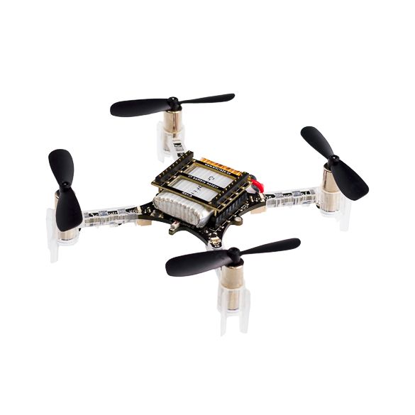
Interacting Swarm Sensing and Stabilization

    Since robotic swarms must operate in real environments, theoretical and experimental swarming
systems have been analyzed in many contexts, including swarms of mobile robots with homogeneous and
heterogeneous agents and delayed communication[32, 33]. Moreover, the dynamics of robotic swarms
have been tested in complex environments, from drones flying in the air, to boats tracking coherent
structures in complex flows, and collaborating robots locating sources in turbulent media[34, 35].
    When deploying swarms in uncertain environments of varying complexity and geometry, it is impor-
tant to understand stability. Recently, we have analyzed stability of swarms in various configurations.
For example, we have studied swarms with complex network topology, and quantified instabilities aris-
ing from heterogeneous topology in the number of local interactions each agents has[36]. We have
examined the effects of communication delay and how environmental noise destabilizes self-organized
patterns[37, 38]. In addition, we have analyzed other environmental effects, such as range-dependent
communication and surface geometry, as a function swarm control parameters [39, 40].
    In all of the above–mentioned research we have considered only a single swarm and its stability in
complex environments. Here we extend our analysis to multiple, interacting swarms, and their resulting
patterns. The general model that we use to describe the dynamics of both single and interacting swarms
contains self-propulsion, friction, and gradient-forces between agents:
                                                            X
                               r̈i = αi − β|ṙi |2 ṙi − λi

                                                              ∂ri U (|rj − ri |)                      (1)
                                                           j6=i

where ri is the position-vector for the ith agent in two spatial dimensions, αi is a self-propulsion
constant, β is a damping constant, and λi is a coupling constant[41, 42, 43, 44]. The total number of
swarming agents is N , and each agent has unit mass. Beyond providing a basis for theoretical insights,
Eq.(1) has been implemented in experiments with several robotics platforms including autonomous
ground, surface, and aerial vehicles[32, 33, 40]. We remark that Eq. (1) contains most of the relevant
physics needed to model an enormous class of behaviors.Moreover, additional physics, stochastic effects,
and network communication topologies may all be added to match many experiments.
    In this paper, we restrict ourselves to the well-known interaction Morse potential, U , which controls
local attraction and repulsion length scales between interacting agents:

                                           U (r) = Ce−r/l − e−r .                                     (2)

2.0    THE GEOMETRY AND DYNAMICS OF COLLIDING SWARMS
We use Eq.(1) to model two interacting swarms with the same underlying dynamics but different
parameters and initial conditions. The most straightforward collision scenario consists of two flocks
colliding, where each swarm has achieved velocity consensus well before collision. The initial distance,
D, which separates the swarms is large enough so that the interaction forces between the swarms are
exponentially small, and θ defines the interaction angle. (See Fig. 1.) The potential function of the
Morse potential is defined by
where C, l define the repulsion and length constants respectively, and the attraction length constant is
scaled to unity.
    Given the initial flocking state configurations, there are three possible final states of the combined
interactions, shown in Fig. 2; i.e., flocking where the swarms combined to form a translating state,
milling where the combined center of mass is stationary, or scattering where the swarms pass through
each other and flock in different directions.

8-2                                                                                      STO-MP-SCI-341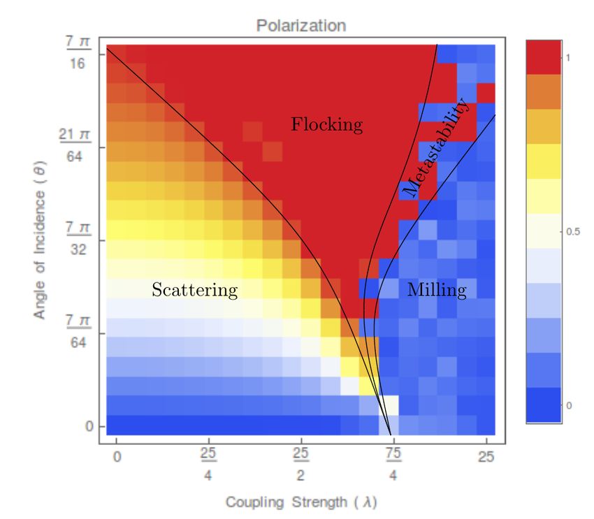
Interacting Swarm Sensing and Stabilization

                     Figure 1: The geometry of two colliding swarms. The initial
                     configurations are flocking states, which intersect at an angle θ.

                Figure 2: Possible final combined configurations of colliding swarm: flocking
                states (left), milling states (middle), and scattering states (right).

   A useful quantity for distinguishing between the three possibilities is the polarization, P, given by
                                                  P
                                                 | i r˙i |
                                            P=   P          .                                        (3)
                                                   i |r˙i |

When the agents are in alignment, P ≈ 1, and it is approximately zero when they are ani-parallel.
Therefore, when the swarms are in the flocking state, P ≈ 1, while in the milling state, P ≈ 0. When
the swarm is in the scattering state it is between 0 and 1. The polarization has been used to quantify
the parameter space comparing angle θ against the coupling strength λi = λ in Fig. 2. We notice that
there exist distinct regions in parameter space where the milling state exists, as well as other regions
show the existence of scattering and flocking.

3.0    THE MILLING STATE - STOPPING COLLIDING SWARMS
We now wish to concentrate on how one swarm may capture another into a combined milling state
where the combined center of mass is stationary and the polarization is close to zero. To satisfy the
latter, θ must be relatively small so that the total momentum is near zero. We make a new diagram
showing exactly where the scattering-to-milling transition occurs for small θ as a function of coupling
λ; an example is shown in Fig. 4. The stable swarm states after collision are specified with blue and
red for scattering and milling, respectively; the green portions indicate the formation of a combined
flocking state, which is comparatively infrequent for small θ (and decreases in frequency as N → ∞).
    In addition, in the right panel of Fig. 4, we show an example of the approach to the milling state as
a series of time snapshots. Initially, the swarms are far apart in flocking states with constant velocities.
As the two swarms approach, however, each agent begins to sense the forces of intra-agent swarmers,
causing the two swarms to rotate around each other while maintaining an approximately constant

 STO-MP-SCI-341                                                                                        8-3
Interacting Swarm Sensing and Stabilization
Figure 3: Polarization as a function of collision angle θ and coupling strength λ.
See [45] for details and parameter values.
inter-swarm density. Over time the two swarms slowly relax to a well-mixed milling state composed of
uniformly distributed agents from both.
Motivated by Fig. 4, one useful observation that can be made regarding the swarms is that, when
flocking towards a collision, each swarm behaves as a rigid body. Assuming such motion in the swarms
leads one to hypothesize that there exists a constant density approximation when all agents have
the same characteristics. Such an approximation can used to create a theory for the center-of-mass
dynamics describing the approach to a milling state, as shown in [46]. In the left panel of Fig. 5, the
center of mass dynamics for each swarm is shown at the critical coupling, λmin : the smallest coupling,
over all collision angles, at which a milling state is stably formed.
7 6
5
0.09 Scatter 4
3 flock 2
flock 1 2
0.07 1
-1 0
time 1 time 2
collision -6 -2 2 6 -3 -1 1 3
0.05
angle Mill 4 4
0.03 3 3
mill
2 2
0.01
1 1
time 3 time 4
0.0 0.2 0.4 0.6 0.8 1.0
critical -3 -1 1 3 -3 -1 1 3
coupling strength
Figure 4: Two swarms colliding. A scattering diagram is shown on the left that specifies the outcome of two-
swarm collisions as a function of the incidence angle and the coupling strength. On the right are four time
snapshots of the swarms at the critical point– the minimum coupling, λmin, at which a collision results in a mill.
Swarm parameters are α = 1, β = 5, C = 10/9, l = 0.75, and N = 100.
The constant density theory predicts that in order for the milling state to occur, the dynamics
must approach a stable limit cycle of the interacting centers of mass. Within this approximation, the
critical coupling corresponds to a generic saddle-node bifurcation. In general, the limit cycle acts as
a capture radius, whereby the two interacting flocks slowly converge to a common, stationary center
The same theory can be used to predict the maximum size of the transient center-of-mass oscillations
as a function of the repulsive coupling, C. In the right panel of Fig. 5 the theory is plotted against
8-4 STO-MP-SCI-341Interacting Swarm Sensing and Stabilization
Figure 5: Collision dynamics resulting in milling. (a) Center-of-mass trajectories for two colliding swarms when λ
= λmin, shown with solid-blue and dashed-red lines. Arrows give the direction of motion. The dashed-black line
indicates the bifurcating limit cycle in the uniform constant density approximation. Other swarm parameters are
α = 1, β = 5, l = 0.75, N = 100, and C = 1.0. The inlet panel shows the corresponding trajectory for λ = 2λmin. (b)
Maximum x-coordinate reached by the center of mass of the rightward moving (blue) flock when λ = λmin.
Simulation results are shown with blue circles for l = 0.75, green diamonds for l = 0.6, and red squares for l = 0.5.
Limit-cycle predictions from theory are drawn with lines near each series. Other swarm parameters are α = 1, β =
5, and N = 200.
numerical simulations to show how well the predictions work for a range of different repulsive-force
strengths.
4.0 ANALYSIS AND FINAL RESULTS OF SWARM SYMMETRY AND
ASYMMETRY
One interesting aspect of the theory is that it can provide a range of parameter predictions for the
critical coupling, λmin , when the swarms are both symmetric and asymmetric. In particular, from the
theory one can define the critical parameter for the saddle-node bifurcation via an equation analogous
to an escape-velocity relation,
v 2 /2 − N λmin Veff (C, l) = 0, (4)
where v is the speed of each flock, and Veff (C, l) quantifies the strength of the potential between agents
(see [46] for full mathematical details). In terms of scaling Eq.(4) implies that, if the potential-forces
and number of agents are held constant, flocks moving twice as fast require√four times the coupling in
order to capture. Similarly, flocks with twice as many particles must fly 2-times faster in order to
escape capture.
We can use the theory to example how the velocity and potential function define the critical cou-
pling λmin as we sweep physical swarm parameters. Examples are shown in Fig. 6. In the left subplot
we show results for collisions with symmetric parameters. Our predicted scaling collapse holds. Quali-
tatively, the critical coupling increases monotonically with C, implying that the stronger the strength
of repulsion, the larger the coupling needs to be in order for colliding swarms to form a mill. Also, note
that our predictions are fairly robust to heterogeneities in the numbers in each flock, particularly for
smaller values of C/l − 1; predictions remain accurate for number asymmetries in the flocks as large
as 20%. In the right panel, we consider how theory compares in the asymmetric case of two swarms
with different velocities. In particular, agents in one flock have self-propulsion αi = α(1) = 1, while
STO-MP-SCI-341 8-5Interacting Swarm Sensing and Stabilization
Figure 6: Critical coupling for forming milling states upon collision. (Left panel) Symmetric parameter collisions
for α = 1 (blue) and α = 2 (red): N = 10 (squares), N = 20 (diamonds), N = 40 (circles), and N = 100 (triangles).
Green stars denote α = 1 and magenta x’s denote α = 2, when 40 agents collide with 60. (Right panel) Asymmetric
collisions for C = 10/9 in which α(1) = 1. Blue points indicate equal numbers in each flock: N = 20 (diamonds), N =
40 (circles), and N = 100 (triangles). Green stars denote collisions between 40 agents with α(1) = 1 and 60 agents
with α(2). Solid and dashed lines indicate theoretical predictions. Other swarm parameters are β = 5 and l = 0.75.
αi = α(2) is varied for the other flock. Again we see that when two swarms come together at the critical
coupling; the results between bifurcation theory and simulations agree well.
5.0 PRELIMINARY COLLIDING SWARM EXPERIMENTS
We have begun to test our theoretical predictions in colliding swarm experiments, where we imple-
mented a mixed-reality setup[32, 33]. To verify the presented theoretical model we used up to eight
Crazyflie micro-UAVs, shown in Fig. 7(b); however eight is an insufficient number of robots to see
meaningful interaction between two large intersecting swarms. To help increase the number of agents
that were used during experimentation we used mixed reality to couple real and virtual robots[47]. In
running the experiments, we used a dimensional version of the Morse potential given by
−|ri −rj | −|ri −rj |
U (ri , rj ) = cr e lr − ca e la . (5)
where cr is the repulsion strength and lr is the length scale of the repulsion; likewise ca is the attraction
strength and la is the attraction length scale.
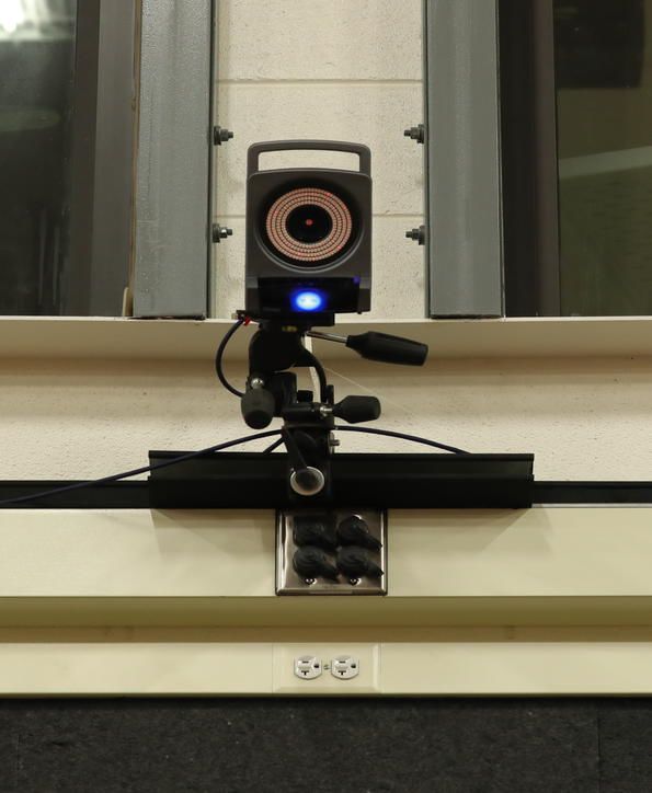
The mixed reality system shown in Fig. 7(a) uses a Vicon motion capture system in a 15x15m
room with between 5-8 Crazyflie micro UAV. The robots positions are shared through a ground station
which also runs the simulation. All agents positions are combined on the ground station and new
positions for the real robots are determined by using a double integrator model of the agents. Figure
8(a) demonstrates how the physical robots interact with simulated agents. The simulated agents, red
dots, are projected into the real world using a camera calibration and the real agents are highlighted
by blue circles. These results allow for further improvement of theoretical predictions and increase
preparedness for field experimentation.
Further examples of mixed reality experiments of two colliding swarms forming a milling state
with a stationary center of mass are shown in Figure 8. In addition to eight real robots vs. eight
simulated robots and see a mill form, we consider even more agents where there are 5 real robots with
8-6 STO-MP-SCI-341Interacting Swarm Sensing and Stabilization
Motion Capture System
Processes on Ground Station
Ground Truth
Position Data
Robots
Simulation
Controller
N Simulated
Robots
Velocity
command for
real robots
(a) Mixed Reality Setup (b) Micro-UAV
Figure 7: In Figure 7(a) a mixed reality experimental platform is shown, which relies on each agent real
and simulated having a global position and receiving some control command. In Figure 7(b) an example of
the Crazyflie 2.0 Micro-UAV, which is used with the Crazyswarm Software. [48].
45 simulated robots versus 50 simulated robots. Due to the inclusion of physical agents which require
space between them it is necessary to consider larger repulsion parameters, cr and lr , to ensure robot
safety. It is clear that even when these values are changed that experimentally a stationary mill is
observed.
Although preliminary, the results show that when the theory is translated to experiments, we can
have one swarm capture another based on the physical parameters chosen. Conversely, our theory
and experiment should also predict when colliding swarms will not form a milling state; i.e., based on
known parameters and sizes of the swarms, we can show one swarm cannot capture another. Other
measures beyond the polarization of how the colliding swarms mix can also be ascertained; one such
metric of measuring the scaling of the density of one swarm with respect to another is presented in the
Appendix A for the mixed reality experiments.
6.0 CONCLUSION AND DISCUSSION
Here we studied the collision of two swarms with nonlinear interactions, and focused in particular on
predicting when such swarms would combine to form a mill. Unlike the full final-scattering diagram,
which depends on whether or not a particular set of initial conditions falls within the high-dimensional
basin-of-attraction for milling – a hard problem in general, we concentrated on predicting the minimum
coupling needed to sustain a mill after the collision of two flocks. By noticing that colliding swarms,
which eventually form a mill, initially rotate around a common center with an approximately constant
density, we were able to transform the question of a critical coupling into determining the stability
of limit-cycle states within a rigid-body approximation. This approach produced predictions that
were independent of initial conditions (only depending on physical swarm parameters) and provided a
lower-bound on the critical coupling for small collision angles. For example, in the case of symmetric
flocks with equal numbers and physical parameters, the scatter-mill transition point was similar to an
escape-velocity condition in which the critical coupling scaled with the squared-speed of each flock, and
inversely with the number of agents in each flock. Our bifurcation analysis agreed well with many-agent
STO-MP-SCI-341 8-7Interacting Swarm Sensing and Stabilization
t = 0.0s t = 15.5s t = 30.0s t = 60.0s
(a) Eight real and eight virtual robots
t = 0.0s t = 15.5s t = 30.0s t = 60.0s
(b) High Repulsion
Figure 8: An example of two time series mixed reality experiments. Figure 8(a) shows 8 virtual colliding with 8
real robots. Figure 8(b) shows an experiment in which 5 real robots join with 45 simulated robots to
collide with 50 simulated robots.
simulations.
Recent work in swarm robotics and autonomy has begun to address how one swarm can detect,
redirect, capture, or defend itself against another[49, 50, 51]. However, most approaches are algorithmic
and lack basic physical and analytical insights. Our work fits nicely into the robotic swarm capture and
redirect problem, since the critical coupling sets a general divide in parameter space between scattering
and milling swarms operating with general physical interactions and dynamics. In this paper, however,
we have not included the effects of communication delays or internal and external noise effects, which
play a significant role in swarms of mobile robots[33, 32]. For example, it is known that when the center
of mass of a single swarm is stationary, time delays in communication can result in stable oscillations
in the center of mass itself. The oscillations are the result of a general delay-induced Hopf bifurcation.
On the other hand, it is also known that (even) small amounts of noise can act as a force, inducing
large changes in swarm behavior[52]. Such large fluctuations may happen in the case where there are
multiple attractors for the center of mass of two interacting swarms. In such cases, noise “kicks" the
center of mass from one attractor to another. For these and other scenarios, new theory and potential
controls will have to be developed using some of the techniques we have presented here to model how
one flocking swarm can capture another.
REFERENCES
[1] Guy Theraulaz, Eric Bonabeau, Stamatios C. Nicolis, Ricard V. Solé, Vincent Fourcassié, Stéphane
Blanco, Richard Fournier, Jean-Louis Joly, Pau Fernández, Anne Grimal, Patrice Dalle, and Jean-
Louis Deneubourg. Proc. Natl. Acad. Sci. U.S.A, 99(15):9645–9649, 2002.
8-8 STO-MP-SCI-341Interacting Swarm Sensing and Stabilization
[2] Chad M. Topaz, Maria R. D’Orsogna, Leah Edelstein-Keshet, and Andrew J. Bernoff. Locust
dynamics: Behavioral phase change and swarming. PLoS Comput. Biol., 8(8):1–11, 08 2012.
[3] A.A. Polezhaev, R.A. Pashkov, A. I. Lobanov, and I. B. Petrov. Int. J. Dev. Bio., 50:309, 2006.
[4] Jinchao Li and Ali H. Sayed. Modeling bee swarming behavior through diffusion adaptation with
asymmetric information sharing. EURASIP Journal on Advances in Signal Processing, 2012(1):18,
Jan 2012.
[5] George F. Young, Luca Scardovi, Andrea Cavagna, Irene Giardina, and Naomi E. Leonard. Star-
ling flock networks manage uncertainty in consensus at low cost. PLoS Comput. Biol., 9:1–7, 01
2013.
[6] M. Ballerini, N. Cabibbo, R. Candelier, A. Cavagna, E. Cisbani, I. Giardina, V. Lecomte, A. Or-
landi, G. Parisi, A. Procaccini, M. Viale, and V. Zdravkovic. Proc. Natl. Acad. Sci. U.S.A,
105(4):1232–1237, 2008.
[7] Andrea Cavagna, Lorenzo Del Castello, Irene Giardina, Tomas Grigera, Asja Jelic, Stefania Melillo,
Thierry Mora, Leonardo Parisi, Edmondo Silvestri, Massimiliano Viale, and Aleksandra M. Wal-
czak. Flocking and turning: a new model for self-organized collective motion. Journal of Statistical
Physics, 158(3):601–627, Feb 2015.
[8] KolbjÞrn TunstrÞm, Yael Katz, Christos C. Ioannou, Cristián Huepe, Matthew J. Lutz, and
Iain D. Couzin. PLoS. Comput. Biol., 9(2):1–11, 2013.
[9] Daniel S Calovi, Ugo Lopez, Sandrine Ngo, Clément Sire, Hugues Chaté, and Guy Theraulaz.
New Journal of Physics, 16(1):015026, 2014.
[10] Kevin Rio and William H. Warren. The visual coupling between neighbors in real and virtual
crowds. Transportation Research Procedia, 2:132 – 140, 2014. The Conference on Pedestrian and
Evacuation Dynamics 2014 (PED 2014), 22-24 October 2014, Delft, The Netherlands.
[11] Frank Cichos, Kristian Gustavsson, Bernhard Mehlig, and Giovanni Volpe. Machine learning for
active matter. Nature Machine Intelligence, 2(2):94–103, 2020.
[12] T. Vicsek and A. Zafeiris. Phys. Rep., 517:71, 2012.
[13] M. C Marchetti, J. F Joanny, S. Ramaswamy, T. B Liverpool, J. Prost, M. Rao, and R. A Simha.
Rev. Mod. Phys., 85:1143, 2013.
[14] M. Aldana, V. Dossetti, C. Huepe, V. M Kenkre, and H. Larralde. Phys. Rev. Letts., 98:095702,
2007.
[15] J. P. Desai, J. P. Ostrowski, and V. Kumar. Modeling and control of formations of nonholonomic
mobile robots. In IEEE Transactions on Robotics and Automation, volume 17(6), pages 905–908,
2001.
[16] A. Jadbabaie, Jie Lin, and A. S. Morse. Coordination of groups of mobile autonomous agents
using nearest neighbor rules. IEEE Transactions on Automatic Control, 48(6):988–1001, June
2003.
STO-MP-SCI-341 8-9Interacting Swarm Sensing and Stabilization
[17] H. G. Tanner, A. Jadbabaie, and G. J. Pappas. Stable flocking of mobile agents part ii: dy-
namic topology. In 42nd IEEE International Conference on Decision and Control (IEEE Cat.
No.03CH37475), volume 2, pages 2016–2021 Vol.2, Dec 2003.
[18] H. G. Tanner, A. Jadbabaie, and G. J. Pappas. Stable flocking of mobile agents, part i: fixed topol-
ogy. In 42nd IEEE International Conference on Decision and Control (IEEE Cat. No.03CH37475),
volume 2, pages 2010–2015 Vol.2, Dec 2003.
[19] V. Gazi. Swarm aggregations using artificial potentials and sliding-mode control. IEEE Transac-
tions on Robotics, 21(6):1208–1214, Dec 2005.
[20] H. G. Tanner, A. Jadbabaie, and G. J. Pappas. Flocking in fixed and switching networks. IEEE
Transactions on Automatic Control, 52(5):863–868, May 2007.
[21] R. Siegwart, I.R. Nourbakhsh, and D. Scaramuzza. Autonomous Mobile Robots. MIT Press,
London, 2011.
[22] I. D. Miller, F. Cladera, A. Cowley, S. S. Shivakumar, E. S. Lee, L. Jarin-Lipschitz, A. Bhat,
N. Rodrigues, A. Zhou, A. Cohen, A. Kulkarni, J. Laney, C. J. Taylor, and V. Kumar. Mine
tunnel exploration using multiple quadrupedal robots. IEEE Robotics and Automation Letters,
5(2):2840–2847, 2020.
[23] D. Pickem, P. Glotfelter, L. Wang, M. Mote, A. Ames, E. Feron, and M. Egerstedt. The rob-
otarium: A remotely accessible swarm robotics research testbed. In 2017 IEEE International
Conference on Robotics and Automation (ICRA), pages 1699–1706, 2017.
[24] E. Kagan, N. Shvalb, and I. Ben-Gal. Autonomous Mobile Robots and Multi-Robot Systems:
Motion-Planning, Communication, and Swarming. Wiley, Hoboken, NJ, 2020.
[25] Ragesh K. Ramachandran, Karthik Elamvazhuthi, and Spring Berman. An Optimal Control
Approach to Mapping GPS-Denied Environments Using a Stochastic Robotic Swarm, pages 477–
493. Springer International Publishing, Cham, 2018.
[26] H. Li, C. Feng, H. Ehrhard, Y. Shen, B. Cobos, F. Zhang, K. Elamvazhuthi, S. Berman, M. Haber-
land, and A. L. Bertozzi. Decentralized stochastic control of robotic swarm density: Theory, sim-
ulation, and experiment. In 2017 IEEE/RSJ International Conference on Intelligent Robots and
Systems (IROS), pages 4341–4347, Sep. 2017.
[27] S. Berman, A. Halasz, V. Kumar, and S. Pratt. Bio-inspired group behaviors for the deployment
of a swarm of robots to multiple destinations. In Proceedings 2007 IEEE International Conference
on Robotics and Automation, pages 2318–2323, April 2007.
[28] M. Ani Hsieh, Ádám Halász, Spring Berman, and Vijay Kumar. Biologically inspired redistribution
of a swarm of robots among multiple sites. Swarm Intelligence, 2(2):121–141, Dec 2008.
[29] Wai Kit Wong, Shujin Ye, Hai Liu, and Yue Wang. Effective Mobile Target Searching Using
Robots. Mobile Networks and Applications, 2020.
[30] Hoam Chung, Songhwai Oh, David Hyunchul Shim, and S. Shankar Sastry. Toward robotic sensor
webs: Algorithms, systems, and experiments. Proceedings of the IEEE, 99(9):1562–1586, 2011.
8 - 10 STO-MP-SCI-341Interacting Swarm Sensing and Stabilization
[31] Ulf Witkowski and Mohamed El Habbal. Ad-hoc network communication infrastructure for multi-
robot systems in disaster scenarios. 6th Framework program of European Union.
[32] Klementyna Szwaykowska, Ira B Schwartz, Luis Mier-y-Teran Romero, Christoffer R Heckman,
Dan Mox, and M Ani Hsieh. Collective motion patterns of swarms with delay coupling: Theory
and experiment. Physical Review E, 93(3):032307, 2016.
[33] Victoria Edwards, Philip deZonia, M. Ani Hsieh, Jason Hindes, Ioana Triandaf, and Ira B.
Schwartz. Delay induced swarm pattern bifurcations in mixed reality experiments. Chaos,
30:073126, 2020.
[34] Hadi Hajieghrary, M Ani Hsieh, and Ira B Schwartz. Multi-agent search for source localization in
a turbulent medium. Physics Letters A, 380(20):1698–1705, 2016.
[35] Christoffer R Heckman, Ira B Schwartz, and M Ani Hsieh. Toward efficient navigation in uncertain
gyre-like flows. The International Journal of Robotics Research, 34(13):1590–1603, 2015.
[36] Jason Hindes, Klementyna Szwaykowska, and Ira B. Schwartz. Hybrid dynamics in delay-coupled
swarms with "mothership" networks. PHYSICAL REVIEW E, 94:032306, 2016.
[37] Klementyna Szwaykowska, Ira B Schwartz, and Thomas W Carr. State transitions in generic
systems with asymmetric noise and communication delay. In 2018 11th International Symposium
on Mechatronics and its Applications (ISMA), pages 1–6. IEEE, 2018.
[38] YN Kyrychko and IB Schwartz. Enhancing noise-induced switching times in systems with dis-
tributed delays. Chaos: An Interdisciplinary Journal of Nonlinear Science, 28(6):063106, 2018.
[39] Jason Hindes, Victoria Edwards, Sayomi Kamimoto, George Stantchev, and Ira B. Schwartz.
Stability of milling patterns in self-propelled swarms on surfaces. Physical Review E, 102:022212,
2020.
[40] Jason Hindes, Victoria Edwards, Sayomi Kamimoto, Ioana Triandaf, and Ira B Schwartz. Unstable
modes and bistability in delay-coupled swarms. Physical Review E, 101(4):042202, 2020.
[41] H. Levine, W. J. Rappel, and I. Cohen. Phys. Rev. E, 63:017101, 2000.
[42] U. Erdmann, W. Ebeling, and A. S. Mikhailov. Phys. Rev. E, 71:051904, 2005.
[43] M. R D’Orsogna, Y. L Chuang, A. L Bertozzi, and L. S Chayes. Phys. Rev. Lett., 96:104302, 2006.
[44] L. Mier y Teran-Romero, E. Forgoston, and I. B. Schwartz. Coherent pattern prediction in swarms
of delay-coupled agents. IEEE Transactions on Robotics, 28(5):1034–1044, Oct 2012.
[45] Carl Kolon and Ira B Schwartz. The dynamics of interacting swarms. arXiv preprint
arXiv:1803.08817, 2018.
[46] Jason Hindes, Victoria Edwards, M. Ani Hsieh, and Ira B. Schwartz. Critical transition for
colliding swarms, 2021.
[47] Klementyna Szwaykowska, Ira B. Schwartz, Luis Mier-y Teran Romero, Christoffer R. Heckman,
Dan Mox, and M. Ani Hsieh. Collective motion patterns of swarms with delay coupling: Theory
and experiment. Phys. Rev. E, 93:032307, Mar 2016.
STO-MP-SCI-341 8 - 11Interacting Swarm Sensing and Stabilization
[48] James A. Preiss*, Wolfgang Hönig*, Gaurav S. Sukhatme, and Nora Ayanian. Crazyswarm:
A large nano-quadcopter swarm. In IEEE International Conference on Robotics and Automa-
tion (ICRA), pages 3299–3304. IEEE, 2017. Software available at https://github.com/USC-
ACTLab/crazyswarm.
[49] H. Park, Q. Gong, W. Kang, C. Walton, and I. Kaminer. Observability analysis of an adversarial
swarmâ a cooperation strategy. In 2018 IEEE 14th International Conference on Control and
Automation (ICCA), pages 992–997, June 2018.
[50] V. S. Chipade and D. Panagou. Herding an adversarial swarm in an obstacle environment. In
2019 IEEE 58th Conference on Decision and Control (CDC), pages 3685–3690, 2019.
[51] V. S. Chipade and D. Panagou. Multi-swarm herding: Protecting against adversarial swarms. In
2020 59th IEEE Conference on Decision and Control (CDC), pages 5374–5379, 2020.
[52] B. Lindley, L. Mier-y-Teran-Romero, and I. B. Schwartz. Noise induced pattern switching in
randomly distributed delayed swarms. In 2013 American Control Conference, pages 4587–4591,
2013.
[53] Benoit Mandelbrot. How Long Is the Coast of Britain? Statistical Self-Similarity and Fractional
Dimension. Science, 156(3775):636–638, May 1967.
APPENDIX A
In addition to polarization to quantify the nature of the milling state, it is useful to find how one
swarm embeds itself in another. One possible way to achieve this is to compute the local density of
the swarm with respect to another. To evaluate the level of interaction between the two swarms we
consider that for all agents in swarm A we compute the following using swarm B:
XX
γ(r) = f (ai , r, bj ), (6)
i∈A j∈B
where f (ai , r, bj ) is defined as follows:
(
||ai − bj || < r 1
f (ai , r, bj ) = (7)
||ai − bj || ≥ r 0,
where r is the radius of inclusion.
8 - 12 STO-MP-SCI-341Interacting Swarm Sensing and Stabilization
Figure 9: The plot shows how the γ(R) changes as a function of ball size radius R. The value of
repulsion constant cr is varied between 1.0 − 5.5 and fixed the repulsion length scale to be lr = 0.1.
This metric is calculating how many agents of a different swarm are in a local neighborhood. It can
be shown γ(r) is related to the fractal or capacity dimension[53]. By varying the radius of inclusion,
one can see how the relative density varies, as shown in Fig. 9. Notice that there exists an inertial
range where γ(R) exhibits roughly linear behavior, which signifies a scale invariant local density of one
swarm relative to another. We find that the mean slope in the inertial region is µ = 1.59 ± 0.19. The
slope reflects a dimension that is fractal, which implies that the agents of one swarm are embedded in
another in a complicated way.
STO-MP-SCI-341 8 - 13Interacting Swarm Sensing and Stabilization 8 - 14 STO-MP-SCI-341
You can also read