Incorporating environmental covariates into a Bayesian stock production model for the endangered Cumberland Sound beluga population
←
→
Page content transcription
If your browser does not render page correctly, please read the page content below
Vol. 48: 51–65, 2022               ENDANGERED SPECIES RESEARCH
                                                                                                    Published May 24
 https://doi.org/10.3354/esr01186               Endang Species Res

                                                                                                    OPEN
                                                                                                    ACCESS

      Incorporating environmental covariates
  into a Bayesian stock production model for the
endangered Cumberland Sound beluga population
                               Brooke A. Biddlecombe1, 2,*, Cortney A. Watt1, 2
   1
       Freshwater Institute, Fisheries and Oceans Canada, 501 University Crescent, Winnipeg, Manitoba R3T 2N6, Canada
              2
                Department of Biological Sciences University of Manitoba, Winnipeg, Manitoba R3T 2N2, Canada

         ABSTRACT: The Cumberland Sound (CS) beluga (Delphinapterus leucas) population inhabits CS
         on eastern Baffin Island, Nunavut, Canada, and is listed as threatened under the Canadian Spe-
         cies at Risk Act. The population dynamics of CS beluga whales have been modelled in the past,
         but the effect of environmental covariates on these models has not previously been considered.
         An existing Bayesian population model fitted to CS beluga whale aerial survey data from 1990 to
         2017 and harvest data from 1960 to 2017 was modified to include sea ice concentration (ICE) and
         sea surface temperature (SST). ICE and SST were extracted for all years from the CS study area in
         March and August, respectively, and incorporated into the state process component of the state-
         space model. The model resulted in a 2018 population estimate of 1245 (95% credible interval [CI]
         564−2715) whales and an initial population estimate of 5147 (95% CI 1667−8779). Determining sus-
         tainable harvest by calculating the probability of population decline estimated 30% probability of
         decline after 10 yr with a harvest of ~15 whales annually. Compared to the previous model with-
         out environmental covariates, which followed a relatively linear trajectory, our model had more
         noticeable peaks and troughs in the population trend and wider CIs. The model suggested harvest
         levels be reduced by ~7 individuals for a management goal with a low risk of decline. The novelty
         of this approach for beluga whales provides an opportunity for further model development via the
         addition of various other abiotic and biotic variables related to beluga whale ecology.

         KEY WORDS: Beluga · Population dynamics · Sea ice · Sea surface temperature · Bayesian model ·
         Harvest

                   1. INTRODUCTION                              nificantly reduced by commercial whaling between
                                                                1868 and 1939 (Mitchell & Reeves 1981). CS belugas
  Beluga whales Delphinapterus leucas are toothed               are the only beluga population listed as threatened
whales with an extensive history of subsistence use             under the Canadian Species at Risk Act (SARA 2017)
by Inuit in the Arctic which continues today (Richard           and are considered endangered by the Committee
& Pike 1993, Wenzel 2009). Cumberland Sound (CS)                on the Status of Endangered Wildlife in Canada
beluga whales are a separate beluga stock that                  (COSEWIC 2004). This listing makes this a popula-
spends summers in northern CS, commonly aggre-                  tion of interest, as harvest levels can have poten-
gating in Clearwater Fiord (66.6° N, 67.4° W), and the          tially severe impacts on the population trajectory due
rest of the year in the main waters of CS (de March et          to the small current population size, estimated at
al. 2002, 2004, Richard & Stewart 2008, Turgeon et al.          ~1400 individuals from an aerial survey in 2017 (Watt
2012) (Fig. 1). The CS beluga population was sig-               et al. 2021).
                                                                © Fisheries and Oceans Canada 2022. Open Access under Cre-
*Corresponding author: biddlecb@myumanitoba.ca                  ative Commons by Attribution Licence. Use, distribution and re-
                                                                production are unrestricted. Authors and original publication
                                                                must be credited.
                                                                Publisher: Inter-Research · www.int-res.com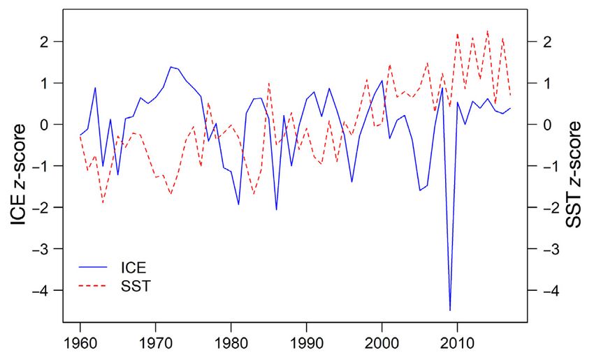
52                                       Endang Species Res 48: 51–65, 2022

                                                                             parameters such as removal level, pre-
                                                                             exploitation population size, or maxi-
                                                                             mum net productivity level (MNPL)
                                                                             and have become an effective way to
                                                                             utilize commonly available data to ad-
                                                                             dress cetacean population dynamics
                                                                             (Baker & Clapham 2004, Wade 2018).
                                                                             Stock assessment models for both fish-
                                                                             eries and marine mammals can be al-
                                                                             tered to include more detail, such as
                                                                             sex and age data (Hilborn & Walters
                                                                             2013, Mosnier et al. 2014), but for
                                                                             many marine mammal populations,
                                                                             these types of data are lacking. While
                                                                             a large amount of information about a
                                                                             population’s past, present, and future
                                                                             can be gained from stock production
                                                                             models, they often do not incorporate
                                                                             other biotic and abiotic aspects of the
                                                                             ecosystem that are potentially impor-
                                                                             tant determinants of population dyna-
Fig. 1. Delineation of Cumberland Sound study area used to clip raster files mics. Typically, these variables are ig-
                                                                             nored for many species because of a
   Population assessments are an important aspect of          lack of data on the relationship between environmen-
species population management because they allow              tal change and population dynamics (Maunder &
population changes to be monitored over time, pro-            Piner 2015).
viding the opportunity to mitigate those changes if              The CS beluga population has been modelled pre-
necessary. Stock production models are a common               viously using a Bayesian state-space model, in-
way of assessing fisheries abundance (Pella & Tom-            formed by historical harvest data and aerial survey
linson 1969, Horbowy 1996, Marcoux & Hammill                  data (Watt et al. 2021). The impact of various har-
2016, Hilborn et al. 2020). A stock production model          vest levels was assessed by calculating the probabil-
analyzes various types of demographic information             ity of population decline in 10 yr. Within a manage-
from a population to determine changes in abun-               ment framework, predicting the effect of various har-
dance from harvest and to project future abundance            vest scenarios on the probability of population
(Maunder & Punt 2013). Stock assessment models                decline is considered a risk-based approach and is
are used for monitoring aquatic populations because           appropriate for evaluating populations that are con-
even if data are lacking, models can still be created         sidered data rich. Data rich in this context is defined
using available information such as catch history,            as having 3 or more abundance estimates within a 15
which often has well-kept records (Maunder & Piner            yr period (Stenson & Hammill 2008). This approach
2015, Best & Punt 2020).                                      allows those involved in population management to
   Marine mammal population assessments began                 make decisions based on the risk of decline they
utilizing techniques from fisheries stock production          deem appropriate. Potential biological removal (PBR)
models in the 1960s, because previous management              is another method for addressing management ob-
methods were resulting in rapid declines of many              jectives, focused on quantifying the number of ani-
cetacean populations (Wade 2018). Although the                mals that can be removed from a stock while allow-
structure is similar, the terminology and output goals        ing a stock to reach or stay at its MNPL after 100 yr
for fisheries versus marine mammal stock production           (Wade 1998). Using the risk-based approach, Watt et
models differ to reflect their different goals. In fish-      al. (2021) suggested that a harvest quota of 20 indi-
eries, stock production models function primarily to          viduals would correspond to a 50% probability of
provide biological reference points to inform quotas          population decline. The priors for this model were
and identify overfishing in stocks (Hilborn & Walters         determined using traditional knowledge, previous
2013, Wade 2018). For marine mammal applications,             cetacean models, and knowledge of cetacean eco-
stock production models are altered to calculate              logy (i.e. Wade 1998, Marcoux & Hammill 2016). As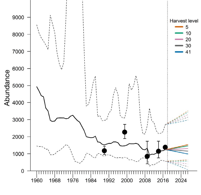
Biddlecombe & Watt: Cumberland Sound beluga population model                          53

with many other cetacean population models (Wade             close association beluga whales have with sea ice
1998, Thomsen et al. 2011, Jacobson et al. 2020), the        (Laidre et al. 2008). Alongside accessing prey that in-
existing CS beluga model lacks detail due to many            habit under-ice areas, sea ice cover acts as refuge
unknowns in beluga demography and did not con-               from killer whale predation (Shelden et al. 2003,
sider how environmental change may be impacting              Bluhm & Gradinger 2008). Due to these associations
the population. There are still many unknowns sur-           with ice, variations in sea ice cover affect beluga
rounding environmental effects on beluga whale sur-          behaviour and have been predicted to affect survival
vival and fecundity (Laidre et al. 2015). Previous           (Kovacs et al. 2011). Sea ice in CS melts in the sum-
cetacean knowledge can provide a basis of knowl-             mer (Maslanik et al. 2011, Yadav et al. 2020), so to
edge for population models, but the lack of reliable         understand the relationship between sea ice and bel-
data impedes the inclusion of details, such as direct        uga whales, sea ice concentration (ICE) values in
effects of an environmental variable on any popula-          winter are more ecologically relevant. In contrast,
tion parameter, into current models. Although direct         summer months do not accurately reflect the condi-
environmental effects are unclear, there is evidence         tion of the ice in a given year. Though studied less
suggesting that changing sea ice dynamics, and sub-          than ICE, SST is another important environmental
sequent changes in food availability, will affect bel-       variable in beluga ecology (Blix & Steen 1979, Aubin
uga whale body condition, and thus population size,          et al. 1990). SST impacts beluga whales because
through negative effects on survival (Laidre et al.          warmer waters promote molting and the proliferation
2008, Choy et al. 2020). Predicted effects are indirect,     of new skin cells and are important for calf thermo-
but there is value in including environmental effects        regulation (Sergeant 1973, Blix & Steen 1979, Aubin
in population models to garner a better understand-          et al. 1990). Calves are born with a thin blubber layer
ing of population-wide effects.                              and thus benefit from a warmer habitat initially until
   Arctic marine ecosystems have undergone rapid             they amass thicker, more insulating blubber. Colder-
change over the past 4 decades (Comiso 2012, Singh           than-usual water in estuaries has been linked to de-
et al. 2013, Parkinson 2014). Climate change has con-        creased survival of beluga calves (Blix & Steen 1979),
tributed to a 4.7% decline in sea ice extent per de-         though this relationship remains understudied. Con-
cade and a decrease of 5 d decade−1 on average in the        versely, increased SST caused by climate change has
length of the sea ice season across the Arctic (Comiso       been predicted to depress calf survival rates, espe-
2012, Parkinson 2014, Yadav et al. 2020). Accompa-           cially alongside other stressors such as reduced prey
nying the loss of sea ice has been a general increase        biomass and increased environmental contaminants
in sea surface temperature (SST) in all regions north        (Williams et al. 2021). Both molting and calving occur
of 60° N (Singh et al. 2013). These environmental            in the summer months, so fluctuations in summer
changes are predicted to affect Arctic marine mam-           SST are likely to have an impact on beluga whales.
mals, although the ability to predict the specific ef-       ICE and SST can have short- and long-term impacts
fects that environmental change will have on popula-         on beluga populations (O’Corry-Crowe 2009, Kovacs
tions is limited (Burek et al. 2008, Laidre et al. 2008,     et al. 2011). Due to sea ice’s connections to refuge
Kovacs et al. 2011). Belugas are expected to be sensi-       from predation, declining sea ice is predicted to have
tive to climate change, influenced by stressors such         short-term effects on mortality; long-term effects are
as ice entrapment — triggered by rapid changes in            more likely to relate to prey availability (such as the
weather, reduced availability of ice-associated prey,        cumulative effects of limited prey consumption) and
and increased predation pressure from killer whales          be difficult to predict (Laidre et al. 2008). Recent
expanding north (Laidre et al. 2008, 2012, Kovacs et         research suggests that changing sea ice dynamics
al. 2011). Most of these predicted effects are indirect,     are already affecting belugas through reduced body
and thus difficult to quantify, and relate to specific as-   condition connected to reduced prey availability
pects of beluga population dynamics. The direct ef-          (Choy et al. 2020). The short-term effects of SST are
fects of sea ice data have been included in a popula-        likely related to calf thermoregulation, as a year with
tion model for harp seals (Hammill et al. 2021), but         unusually low or high summer temperatures could
compared to cetaceans, more data and thus more               affect calf survival and thus have immediate effects
explicitly identified relationships between variables        on population dynamics (Blix & Steen 1979, O’Corry-
and population parameters are available for seals.           Crowe 2009). SST also affects beluga molting (Aubin
   Several environmental variables that have been            et al. 1990); low temperatures may inhibit molting
predicted to affect beluga populations, among them           and cell proliferation, potentially affecting abun-
sea ice extent, are a recurring concern due to the           dance through reduced body condition, but unsuit-
54                                            Endang Species Res 48: 51–65, 2022

able conditions may need to be prolonged before there              growth rate fit to aerial survey data from 1990 to 2017
are notable population-wide effects.                               and harvest history from 1960 to 2017 using Bayesian
  The objective of this study is to incorporate envi-              Markov chain Monte Carlo (MCMC) methods to esti-
ronmental covariates, specifically ICE and SST, into a             mate population dynamics from 1960 to 2017. In this
stock production model to include the effects of envi-             hierarchical state-space model, data are considered to
ronmental variation on estimates of CS beluga popu-                be the outcome of 2 distinct stochastic processes: a
lation trends. Further, we aim to compare models                   state process and an observation process (de Valpine
with and without covariates to determine how the                   & Hastings 2002). The state process arises from un-
inclusion of environmental variables might alter pre-              derlying population dynamics and evaluation of stock
dicted future trajectories and thus population man-                size over time and is a discrete formulation of the
agement plans.                                                     Schaefer (1954) model, which allows both positive
                                                                   and negative effects on growth rate. The state process
                                                                   uses population parameters and error (quantifying
           2. MATERIALS AND METHODS                                random variation in population dynamics) to estimate
                                                                   true population size annually. Population size, Nt , is a
                2.1. Model specification                           function of the previous year’s population:

                                                                                                      N
  The CS beluga stochastic stock production model                          Nt = Nt 1  1+ (Rmax )  1 t 1   p  Rt   (1)
                                                                                                        K
from Watt et al. (2021) was used as a template to in-
corporate the effect of environmental covariates on                where R max is the maximum growth rate or rate of
population dynamics (Fig. 2). The model was struc-                 population increase; K is the environmental carrying
tured with density dependence acting on population                 capacity; εp is a stochastic term for the process error
                                                                                   with environmental covariates; and Rt
                                                                                   is the removals for that year, calcu-
                                                                                   lated as reported catches, CRt , that are
                                                                                   corrected for the proportion of animals
                                                                                   that were struck and lost, S&L:
                                                                                               Rt = CRt × (1 + S&L)         (2)
                                                                                       S&L is also a way to account for
                                                                                    potential under-reporting in catch his-
                                                                                    tory. S&L data themselves can be
                                                                                    under-reported, but because we have
                                                                                    no available S&L data for CS belugas,
                                                                                    we must rely on the prior being in-
                                                                                    formed by data from eastern Hudson
                                                                                    Bay belugas (see Watt et al. 2021).
                                                                                       The observation process is the rela-
                                                                                    tionship between true population size
                                                                                    (Nt) and observed data (St), associated
                                                                                    with random uncertainties, or obser-
                                                                                    vation error (εSt), in data collection and
Fig. 2. Hierarchical state-space population model structure depicting linkages      abundance estimation. The logarithm
between state process (solid grey outline), observation process (dashed grey        of the median Nt estimate from this log-
outline), and harvest (dotted grey outline). Grey circles indicate data, white      normal model is applied to the state
rectangles indicate parameters to be estimated by the model, and black lines
                                                                                    process model described above.
indicate dependencies between parameter and/or data. N: population size;
Rmax: maximum growth rate or rate of population increase; K: environmental                      ln(St) = ln(Nt) + εSt       (3)
carrying capacity; εp: stochastic term for the process error with environmental
covariates; Rt : removals for that year, calculated as reported catches (CR) that     A model of this type would benefit
are corrected for the proportion of animals that were struck and lost (S&L); S:     from the inclusion of age or sex struc-
survey data; εSt: stochastic term for observation error; ICE: mean sea ice con-
centration in Cumberland Sound (CS) in March; SST: mean sea surface tem-            ture, especially considering one of our
perature in CS in August; B: coefficient being estimated by the model for ICE;      chosen covariates, SST, potentially has
              C: coefficient being estimated by the model for SST                   a differing effect based on age. Unfor-
Biddlecombe & Watt: Cumberland Sound beluga population model 55
tunately, our model does not contain information on Similarly, when the same months were tested for ICE
age or sex for this population, as there are no reliable and SST across the year, correlation remained high.
data available at this time. Finally, annual averages were also tested, but using
Included surveys occurred in 1990, 1999, 2014, and all the values within a year dampened the extremes
2017; all surveys were systematic visual in design. in ecologically relevant months that we were aiming
All surveys were adjusted to account for availability to investigate the effects of.
bias, and the 2017 survey was adjusted for percep- We used a 6 × 9 pixel polygon to extract data from
tion bias (as per Watt et al. 2021). the environmental raster files specific to CS (Fig. 1).
The means of all pixels in the resulting clipped raster
files from each year were calculated, and the mean
2.2. Process error incorporating values were translated into a z-score for ICE and SST
environmental covariates separately. z-scores were used in the process error,
so the environmental variables in the model reflected
To capture more of the natural variation within the the variation of each value from the mean for all
population, process error was modified from the pre- years during the study period of 1960 to 2018 (Fig. 3).
vious template model to include the effects of envi- We used a Pearson correlation test to determine if
ronmental variation. ICE and SST were incorporated there was collinearity between ICE and SST and if
into the process error term (see Fig. S1 in the Supple- they could be incorporated into the same model. The
ment at www.int-res.com/articles/suppl/n048p051_ resulting correlation coefficient was −0.12, which is
supp.pdf for details). Both ICE and SST are spa- low enough to allow for the incorporation of both
tially gridded data with a 1° × 1° resolution consist- environmental covariates into the model (Vatcheva &
ing of monthly averages and were obtained from the Lee 2016). We also tested the square of SST in initial
HadISST data set (Rayner et al. 2003). model runs to determine if there was a non-linear
The model requires the process error to have an- relationship, where extreme highs and lows had a
nual values for each covariate, so to avoid the loss of negative impact on population size. The inclusion of
nuance in interannual variation, we chose to use a SST2 decreased model fit and thus was not explored
single month based on ecological significance to bel- further.
ugas, instead of an annual average. We used ICE
data from March of each year from 1960 to 2018, as
March, on average, is the month of highest sea ice ex- 2.3. Priors
tent across the Arctic (Maslanik et al. 2011, Stroeve et
al. 2012). For SST, we used August data, as August, The majority of priors remained the same as those in
on average, is the month with the highest SSTs (Shea the template model (Table 1) from Watt et al. (2021).
et al. 1992, Chambault et al. 2018). We chose ICE and The stochastic process error term εp was altered to in-
SST maximum months a priori based on ecological clude the additive effects of ICE and SST. The equa-
relevance, but we also considered minimum months tion below was used for the location parameter of the
for either variable and intra-annual patterns in ICE process error, with the precision hyperparameter (εpr)
and SST. Months with minimum ICE and SST values,
August and March, respectively, were explored as
well as the same month for both ICE and SST and an-
nual averages. ICE values in August largely reflected
a lack of ice cover, which was not valuable for rep-
resenting environmental variation. SST values in
March were not ecologically applicable to beluga
whales, compared to summer months, as variability
in SST was predicted to have the most impact on bel-
uga whale summer ecology. We decided not to ex-
plore the use of minimum months further, as mini-
mum ICE in August represents a time when sea ice
cover has less ecological importance to belugas; in
addition, minimum SST in March was too highly cor- Fig. 3. Mean sea ice concentration (ICE) in March and mean
related with ICE in March (Pearson correlation coeffi- sea surface temperature (SST) in August as z-score values
cient of −0.97) to be considered independent of ICE. in Cumberland Sound from 1960 to 201756 Endang Species Res 48: 51–65, 2022
Table 1. Prior distributions, parameters, and hyperparameters used in the template population model (from Watt et al. 2021) and
environmental covariates sea ice concentration (ICE) and sea surface temperature (SST) corresponding to the process error
used in the final model. dist.: hyperparameter with its own prior distribution; (−) not applicable to the model
Parameter Notation Prior distribution Hyperparameter Value from Value for model with
Watt et al. (2021) ICE and SST
Survey error (t) εSt Log-normal μs 0 0
τs dist. dist.
Precision (survey) τs Gamma αs 2.5 2.5
βs 0.4 0.4
Process error (t)a εpt Log-normal μp 0 B × ICE + C × SST
τp dist. dist.
Precision (process)a τp Gamma αp 1.5 1.5
βp 0.00005 0.001
ICE coefficienta B Normal μB − 0
τB − 5
SST coefficienta C Normal μC − 0
τC − 5
Struck and lost S&L Beta αsl 3 3
βsl 4 4
Initial populationa N1960 Uniform Nupp 4000 9000
Nlow 1000 1000
Carrying capacity K Uniform Kupp 15 000 15 000
Klow 2000 2000
Lambdaa λ Uniform 0.01−0.05 0.01−0.07
a
Variable differs from or is new to the template model
free to vary to account for error not explained by the with coefficients assigned moderately informed nor-
covariates (see R code details in the Supplement for mal (0, 5) distributions. The model was also re-run
details). with each covariate individually to explore the effect
of each covariate alone.
(εp)t = (B × ICEt−1 + C × SSTt−1) + εpr (4)
The stochastic process error term εp included in the
where ICE is the mean concentration in CS in March, state process equation (Eq. 1) was assigned a log-nor-
SST is the mean temperature in CS in August, B is mal distribution with a location parameter set by the
the coefficient being estimated by the model for ICE, process error equation (Eq. 4) described above. The
C is the coefficient being estimated by the model for precision parameter for the process error term was
SST, t is annual time, and εpr is the random error from assigned a moderately informative gamma(1.5, 0.001)
the process precision parameter. distribution. The precision term within the precision
Both ICE and SST were multiplied by independent parameter was reduced as compared to the precision
coefficients and were autoregressive to an order of 1 parameter in Watt et al. (2021) to allow the opportu-
to allow the model to determine the effect each envi- nity for process error to increase and have more of an
ronmental covariate had on process error and thus effect on interannual variation in the population tra-
population dynamics in the following year. We fo- jectory. Precision for process error was high in the
cused on 1 yr autoregressive effects, although it is Watt et al. (2021) model because, as a long-lived spe-
ecologically plausible that these covariates may have cies, beluga whales were not expected to exhibit a
effects over a greater time span, and this would be high amount of annual stock variation. We decreased
valuable to test in future models. Prior distributions precision to allow the model to explore more varia-
for coefficients were informed by the necessity for tion, to accommodate uncertainty surrounding the
coefficients to fall between −1 and 1. Initial ex- covariates. Initial runs of the model showed that the
ploratory runs were performed with each covariate prior distributions for starting population and Rmax in
alone in the model and with both covariates together. the template model appeared to constrain the poste-
The best fit model included both covariates, both rior distributions. Both parameters had uniform distri-Biddlecombe & Watt: Cumberland Sound beluga population model 57
butions in the template model, so the starting popula- different management scenarios reflecting annual
tion distribution was widened to a uniform (1000− harvests of 5, 10, 20, 30, and 41 individuals. Although
9000) distribution, and Rmax was widened to a uniform a 10 yr trajectory is relatively short, it was chosen be-
(0.01−0.07) distribution (Table 1). The updated start- cause, ideally, harvest quotas for marine mammals
ing population distribution allows space for the model are re-assessed every 5 yr. The current harvest quota
to estimate a slightly higher population in 1960 if nec- is 41 individuals, and because CS belugas are endan-
essary. Rmax in the template model was informed by gered and not predicted to recover at the current
known rates of population increase in odontocetes, quota (Watt et al. 2021), only harvests below the cur-
which can range from 0.02 to 0.06 (Wade & Angliss rent quota were considered for projections. We ex-
1997, Wade 1998, Lowry et al. 2008), which also in- plored how adding environmental covariates changed
formed our prior. the probability of decline from the template model.
To continue the comparison of our model to the
template model from Watt et al. (2021), we estimated
2.4. Parameter estimation and model diagnostics PBR using a recovery factor (F R) of 0.1 for a threat-
ened declining stock (Hammill et al. 2017). The
Posterior estimates for all parameters included in equation for the PBR threshold is:
the model were obtained using a Gibbs sampler
PBR = Nmin × 0.5 × Rmax × F R (5)
algorithm implemented in JAGS (Plummer 2003).
RStudio (R Core Team 2020; version 1.2.5033, R ver- where Rmax is the maximum rate of population in-
sion 4.0.2) packages R2jags (Su & Yajima 2015; ver- crease (the default value for cetaceans is 0.04; how-
sion 0.6-1) and coda (Plummer et al. 2006; version ever, in our calculation, we used the Rmax estimated
0.19-3) were used to examine the results. We used an by the model), FR is a recovery factor (between 0.1
MCMC simulation method and visually inspected and 1), and Nmin is the estimated population size
trace plots to check the convergence of parameters. using the 20th percentile of the posterior distribution
Initial runs of the code investigated model conver- resulting from the model or the 20th percentile of the
gence, mixing, and autocorrelation within para- log-normal distribution (Wade 1998) of the aerial sur-
meters. Model fit was determined using the diagnos- vey estimate.
tics described below and the deviance information Animals that are harvested as well as those that are
criterion (DIC), although DIC did not have a differ- struck and lost (S&L), those that are not reported, and
ence > 2 between any of the models (Burnham & those with other sources of human-caused mortality
Anderson 2002), so other diagnostics assessing con- are all included in PBR estimates; thus, we need to
vergence were used preferentially. estimate total allowable landed catch (TALC), which
We visually inspected Geweke plots to test for mix- is calculated as:
ing within each chain and used the Geweke diagnos-
TALC = PBR − S&L (6)
tic test of similarity between different sections of the
chains (Geweke 1996). The Brooks-Gelman-Rubin where S&L is estimated in the model.
(BGR) diagnostic test was used to validate conver-
gence between chains by comparing the width of the
80% credible interval (CI) of the chains pooled with 3. RESULTS
the mean widths of the 80% CI for each of the chains
individually (Brooks & Gelman 1998). The final CS beluga model, adapted from Watt et
In initial model runs, we used 3 chains which had al. (2021) (Table 2), included ICE for the month of
the number of iterations corrected to equal 10 000 March and SST for the month of August in CS from
after a burn-in of 6000 and thinning value of 30. 1960 to 2017. Differences between results for the 3
Once a top model was determined, that model was models tested (ICE alone, SST alone, and ICE and
run using 5 chains and 100 000 iterations after a SST together) were minimal. DIC and BGR values
burn-in of 60 000, with thinning maintained at 30. were not distinguishable, and convergence of all
parameters was similar. Due to the similarities,
model selection was led by Geweke diagnostic test
2.5. Future projections and management scenarios results, where the z-scores for multiple parameters in
the ICE and SST models were lower than those in
To predict stock trajectory and sustainable yield, models with the covariates alone. The focal update of
the model was extended 10 yr into the future under 5 our final model was the addition of environmental58 Endang Species Res 48: 51–65, 2022 Table 2. Model outputs for the Cumberland Sound (CS) beluga stock model from Watt et al. (2021) and our final model. The mean, SD, median (50th quantile [Q]), 25th Q, 75th Q, and 95% credibility intervals (CIs; 2.5% and 97.5%) are given for the following model para- meters and their priors: carrying capacity (K ), Lambda (1 + Rmax), process error (process), survey precision (surv), starting population (startpop), struck and loss (S&L), and population size in 2018 (N2018). Coefficients for sea ice concentration (ICE; B) and sea surface tem- perature (SST; C ) are included in the final model output. R̂ is the Brooks-Gelman-Rubin statistic; values
Biddlecombe & Watt: Cumberland Sound beluga population model 59
Fig. 4. Model estimates of Cumberland Sound (CS) beluga
abundance fitted to adjusted aerial survey estimates flown
in 1990, 1999, 2009, 2014, and 2017 (black dots ± 95% log-
normal credible interval [CI]) and harvest data from 1960 to
2017. Process error includes the effects of sea ice concentra-
tion and sea surface temperature in CS. Solid line shows the
posterior median estimates, dashed lines show 50% CI, and
dotted lines show 95% CI
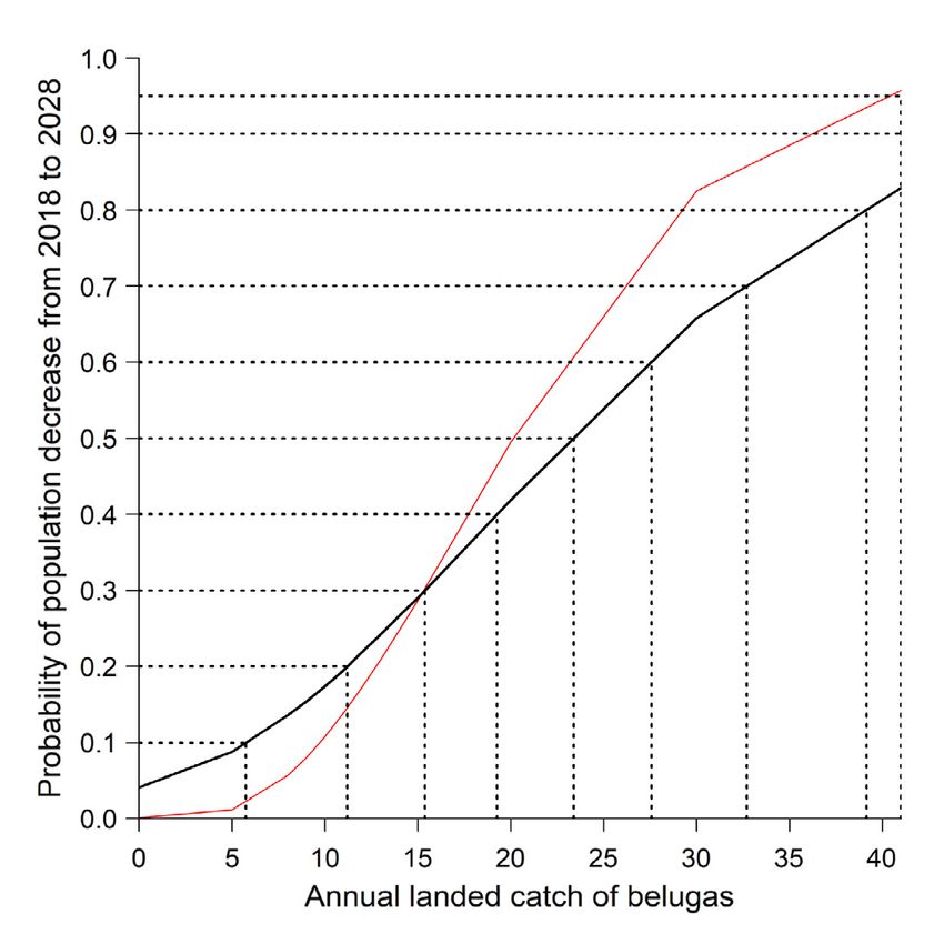
To assess the impacts of different management
strategies on the population, the model was used to
plot the trajectories of 5 harvest scenarios (Fig. 6).
The probability of population decline after 10 yr was
83% for a harvest of 41, 66% for a harvest of 30, 42%
for a harvest of 20, 18% for a harvest of 10, and 9%
for a harvest of 5 (Table 3, Fig. 7). Using the N2018
estimate from the model, the PBR was estimated at 2,
and TALC was estimated at 1 individual.
4. DISCUSSION
Fig. 5. Model estimates of Cumberland Sound (CS) beluga
abundance fitted to adjusted aerial survey estimates flown in
The environmental variables ICE and SST were
1990, 1999, 2009, 2014, and 2017 (black dots ± 95% log-normal
successfully incorporated into the stock production credible interval [CI]) and harvest data from 1960 to 2017. (A)
model for CS belugas. The covariates ICE and SST Process error with the effect of sea ice concentration in CS and
acted on the process error, impacting the CS beluga without sea surface temperature. (B) Process error with the
population trajectory by contributing to some of the effect of sea surface temperature in CS and without sea ice
concentration. Solid line shows the posterior median estimates,
variability in population dynamics. The positive coef- dashed lines show 50% CI, and dotted lines show 95% CI
ficient for ICE means that following a year of above-
average ICE, the beluga population would increase,
and after a below-average year, the beluga population The coefficients for both covariates are small, reflect-
would decrease. Similarly, the positive coefficient for ing a relatively small effect that ICE and SST have on
SST reflects an upward trend in beluga population population trajectory indirectly through process error.
trajectory following a year of above-average SST and Compared to abundance estimates from the template
a downward trend after a year of below-average SST. model (Watt et al. 2021), the largest difference in any60 Endang Species Res 48: 51–65, 2022
Fig. 6. Future population projections for Cumberland Sound
(CS) belugas under 5 different harvest level scenarios based Fig. 7. Probability of the Cumberland Sound (CS) beluga stock
on population estimates from a stochastic stock production decreasing from the 2018 abundance estimate after 10 yr of
model including sea ice concentration and sea surface tem- harvest, as a function of the number of reported belugas re-
perature, fitted to adjusted aerial survey estimates flown in moved from the stock every year (black line). Dotted lines in-
1990, 1999, 2009, 2014, and 2017 (black dots ± 95% log- dicate levels of harvest (x-axis) corresponding to the proba-
normal credible interval [CI]). Solid line shows the posterior bility of decline (y-axis). Red line shows probability of CS
median estimates, and dashed lines show 95% CI beluga stock decrease from template model (Watt et al. 2021)
Table 3. Probability that the Cumberland Sound beluga pop- ICE is 3 times larger than the coefficient for SST;
ulation, subjected to different levels of annual landed catch, therefore, in most years, ICE will have a greater ef-
will decline from the modelled 2018 population abundance
fect on population fluctuations than SST. In years
estimate after 10 yr of harvest. Comparing results from Watt
et al. (2021) and our final model (with sea ice concentration where the value for either covariate has a high devi-
[ICE] and sea surface temperature [SST]) ation from the mean, that covariate had a stronger
effect on population fluctuations. The greatest uncer-
Landed catch p (%) p (%) with tainty in the population estimate is at the peak in the
Watt et al. (2021) ICE and SST 97.5th quantile between 1970 and 1985. Aside from
the lack of survey data in early years to bolster esti-
5 1 9 mates, ICE trends were consistently high in CS in the
10 11 18
20 50 42 early 1970s (Fig. 3), and based on the results from the
30 83 66 models where covariates were included separately,
41 96 83 it appears ICE is driving the majority of this un-
certainty. Sea ice is inherently variable; despite clear
downward trends, annual values are found to com-
year was an increase of ~3000 individuals and the monly deviate from the trendline (Cavalieri &
smallest was ~5 individuals. The greatest differences Parkinson 2012). The quantiles for SST alone are
were in years at the beginning of the time series; this smaller, with less variation. SST is potentially more
is likely because there are no available aerial surveys stable over time than sea ice, which is seasonally
before 1990 to inform the trajectory, so during that pe- dependent and susceptible to short-term fluctuations
riod, the covariates have more power to inform trends. (Cavalieri & Parkinson 2012, Carvalho & Wang 2020).
Although the coefficients allude to ICE and SST The combination of consistently above-average ICE
having similar effects on population trajectories, ICE values and relatively low harvest levels in the early
and SST have low correlation, so there is an interac- to mid-1970s could have resulted in the model hav-
tive effect between these covariates and how they ing increased uncertainty in population estimates for
affect the CS beluga population. The coefficient for those years.Biddlecombe & Watt: Cumberland Sound beluga population model 61 The final model contained both covariates, ICE and aid in skin molting (Watts et al. 1991). Calving also SST, but we also tested the independent effects of occurs in the summer, and warmer water likely in- each covariate. While there was a positive effect from creases calf survival by aiding thermoregulation each environmental covariate on the model trajec- (Sergeant 1973, Blix & Steen 1979). The connection tory, similar to our final model, the coefficient was between warmer water and important aspects of bel- lower for both ICE and SST when they were sepa- uga ecology could explain the positive relationship rate. Although they have a notable effect on the pop- between SST and beluga population size determined ulation trajectory alone, when ICE and SST are con- by our model. There is a loose correlation between sidered together, coefficients for both are higher; low SST years and higher ICE, although there is a lot thus, they have a greater effect on the re-creation of of variability within this relationship (Hurrell et al. plausible population fluctuations, suggesting im- 2008), so the lack of correlation in our data between pacts are synergistic. There is also the potential that ICE in March and SST in August in CS is plausible. the larger effect for each covariate when they are Our model uses covariates that are 1 yr autoregres- together is the result of their more extreme values sive and thus focuses on the short-term effects of ICE dampening the effects of each other, as they are not and SST. The model could be altered to consider correlated, or the effect of an unknown confounding long-term effects by increasing the number of years variable acting on both. It is difficult to identify other the model is autoregressive to, resulting in model temporally variable covariates that have known ef- outputs being affected by years further in the past. fects on beluga whale population dynamics because Changing the temporal aspect of the covariate inclu- although important habitat features have been iden- sion provides the potential to show how ICE and SST tified (Laidre et al. 2008), the effect that changes in (or other covariates) affect the population after more those features have on population dynamics has not than 1 yr, which potentially varies from the initial been quantified. The overall trajectories of the sepa- impacts (Gilg et al. 2012). For example, low ICE may rate models have shallower fluctuations than our cause beluga whales to have reduced access to prey, final model. In the final model, the coefficients are but the result of a change in resources may not show greater and therefore have a larger effect on the pro- up in the population for several years. Similarly, if cess error and thus create more fluctuations in trajec- summer SST is lower than average and negatively tory. The inclusion of both covariates is supported affects beluga molting, the effects tied to incomplete ecologically because there is likely interaction be- molting may take a number of years to become quan- tween these variables and how they are affecting tifiable or not even act on population parameters beluga survival (Asselin et al. 2011, Hauser et al. directly. At this time, a lack of data makes it difficult 2017). Unfortunately, the data are still too sparse to to speculate on the time frame over which impacts identify these specific relationships in a population might occur. We started by evaluating a 1 yr time model context, but our model provides support that frame, but additional data may support increasing there is value in evaluating the interaction between the time lag. Hammill et al.’s (2021) harp seal popu- ICE and SST and their effect on beluga populations, lation model utilized mortality data to determine a with the opportunity to expand on these relation- 1 yr time lag for the effect that sea ice anomalies had ships as additional data become available. on the survival of young of the year. Our model could Multiple studies recognize that the environmental be updated with a specific time lag relationship of changes occurring in the Arctic are affecting beluga this nature once more data are available. whales (Laidre et al. 2008, Kovacs et al. 2011), but The inclusion of environmental covariates into our identifying the specific connections to reproduction model resulted in changes to multiple aspects of the and survival is challenging. Belugas are highly ice previous CS beluga model from Watt et al. (2021). associated; they prefer high ice cover (Asselin et al. In comparison to the template CS stock production 2011) and often use ice cover as refuge from preda- model (Watt et al. 2021), the model presented here tion (Stewart & Stewart 1989, Shelden et al. 2003). had a higher starting population estimate, a slightly Declining sea ice can make beluga whales more vul- higher N2018 estimate, and a lower carrying capacity. nerable to predation and reduce access to prey The maximum growth rate increased slightly toward (Heide-Jørgensen & Laidre 2004, Kovacs et al. 2011), the accepted default for cetaceans (Wade 1998), and which explains why our model determined that years S&L increased by 3%. In the template model, the of lower ICE had a negative effect on the CS beluga population decrease over time followed a relatively population trajectory. Beluga whales prefer to in- linear trajectory. However, in our model, there are habit warmer water in the summer, as it is believed to more noticeable peaks and troughs in the popula-
62                                      Endang Species Res 48: 51–65, 2022

tion trend and wider CIs. The resulting increased          dangered status of CS belugas (COSEWIC 2004).
starting population created a previously unobserved        Further research using a Bayesian stock production
trend of steep population decrease early in the study      model could provide clarity on the effects of environ-
period when both ICE and SST were below average            mental covariates on beluga population dynamics and
for many years. This steep trend suggests that when        provide increased confidence in sustainable manage-
the population abundance was higher, it was quite          ment using a risk-based approach.
vulnerable to environmental fluctuations. The higher         Hammill et al. (2021) proposed an age-structured
starting population also suggests that pre-harvest         harp seal population model with sea ice incorporated,
abundance is potentially higher than was suggested         where the specific relationship between sea ice cover
in Watt et al. (2021), although carrying capacity is       anomalies and mortality of young of the year was de-
estimated to be lower by ~2000 individuals. These          fined. Compared to Arctic cetaceans, there are more
differences may need to be considered for future           data available on how covariates such as ice, which is
management goals if density dependence were to             used as a pupping platform, and prey availability af-
act on the population as it approached carrying            fect specific aspects of harp seal population dynamics,
capacity; however, this is unlikely given its current      such as mortality and reproductive rates (Stenson et
population trend and endangered status (COSEWIC            al. 2020, Hammill et al. 2021). While the results of our
2004).                                                     model provide baseline knowledge on the effect of
  We used a risk-based model approach to determine         environmental variation on population fluctuations,
the probability of population decline under potential      there is the potential for the inclusion of much more
management scenarios. Compared to similar risk-            detail in models of this type in the future, as ICE and
based results from Watt et al. (2021), the inclusion of    SST are only 2 of many variables that may affect bel-
environmental covariates decreased the probability         uga population dynamics. Other relevant variables
of decline for the 3 highest harvest scenarios and         may include water depth, seafloor topography, and
increased it for the 2 lowest scenarios. We speculate      distance to important features such as shoreline (As-
this is due to a more stable overall population trend      selin et al. 2011, Hauser et al. 2017). Belugas are
in Watt et al.’s (2021) model (due to less variation in    thought to preferentially select for shallower water for
process error), allowing the population to remain sta-     increased prey availability; similarly, they select for
ble at lower harvest levels. A lower 2018 abundance        regions with a higher seafloor slope, likely due to the
estimate from Watt et al. (2021) may cause high har-       increased productivity resulting from increased up-
vest levels to have a more dramatic effect, bringing       welling in these regions (Asselin et al. 2011). Sus-
abundance so low that population stability is lost. In     pected selection for these static habitat features may
the template model, a harvest of 20 had a ~50% prob-       change depending on changes in dynamic features,
ability of decline; in our model, a 50% probability of     such as ICE, and the interplay between habitat
decline was reached at a harvest level of ~24. How-        change, prey availability, and the presence of preda-
ever, the recommended harvest suggested by our             tors. This model could further benefit from the inclu-
model is slightly more conservative than the harvest       sion of predator and prey dynamics and the inter-
level suggested by Watt et al. (2021) when lower prob-     actions these biotic variables might have with abiotic
abilities of decline are considered. Our model reulted     environmental variables. In this model, the environ-
in a 5% probability of decline over a 10 yr period,        mental covariates were introduced via process error,
with a harvest of ~1, while Watt et al. (2021) found a     yet as beluga whale research progresses, there is the
suggested harvest of ~8 had a 5% probability of            potential for more specific relationships between bel-
decline. Using the 2018 population estimate and the        uga population dynamics and changes in environ-
Rmax of 0.038 from our model, the PBR threshold was        mental parameters to be quantified. An understanding
2. The PBR threshold calculated by Watt et al. (2021),     of the mechanistic relationships would allow environ-
using their 2018 estimate and an Rmax of 0.04, had a       mental covariates to be included into stock production
value of 1. The slight difference between PBR thresh-      models directly rather than within the process error,
olds is likely due to differences in estimated 2018        which would create more certainty in resulting pa-
abundance. The goal of this work is to consider how        rameter estimates. For example, if new data allowed
environmental variables might change our interpre-         us to quantify the relationship between ICE and mor-
tation of population trends and consider whether this      tality from predation, the model could be modified to
ecosystem approach may be used for future assess-          include that direct relationship. ICE and SST impacted
ments. In the face of uncertainty, a more conservative     the CS beluga population trajectory; thus, inclusion of
management strategy is beneficial because of the en-       these variables in future models should be considered
Biddlecombe & Watt: Cumberland Sound beluga population model                                63

to aid in explaining population trajectories of belugas            changing climate: patterns and mechanisms. Global
and other Arctic marine mammals.                                   Planet Change 193:103265
                                                                Cavalieri DJ, Parkinson CL (2012) Arctic sea ice variability
  CS belugas are a threatened population under                     and trends, 1979−2010. Cryosphere 6:881−889
SARA (SARA 2017) and considered endangered by                   Chambault P, Albertsen CM, Patterson TA, Hansen RG,
COSEWIC (COSEWIC 2004), and it is important to                     Tervo O, Laidre KL, Heide-Jørgensen MP (2018) Sea sur-
consider this status when making decisions on mod-                 face temperature predicts the movements of an Arctic
                                                                   cetacean: the bowhead whale. Sci Rep 8:9658
elling, management, and conservation. Including cli-
                                                                Choy ES, Giraldo C, Rosenberg B, Roth JD and others (2020)
mate and habitat changes that are affecting endan-                 Variation in the diet of beluga whales in response to
gered species is important for conservation research               changes in prey availability: insights on changes in the
because in many cases, climate change is shifting the              Beaufort Sea ecosystem. Mar Ecol Prog Ser 647:195−210
                                                                Comiso JC (2012) Large decadal decline of the arctic multi-
baselines that guide conservation goals (Wilkening
                                                                   year ice cover. J Clim 25:1176−1193
et al. 2019, Hirsch 2020). Many endangered species              COSEWIC (Committee on the Status of Endangered
are specialists, endemic to their habitat, making                  Wildlife in Canada) (2004) COSEWIC assessment and
them likely to be disproportionately affected as their             update status report on the beluga whale Delphi-
habitat changes (Preston et al. 2008, Gough et al.                 napterus leucas in Canada. Committee on the Status of
                                                                   Endangered Wildlife in Canada, Ottawa
2015, Wilkening et al. 2019). A certain level of uncer-         de March B, Maiers L, Friesen M (2002) An overview of
tainty is almost always involved in endangered spe-                genetic relationships of Canadian and adjacent popula-
cies management (Gregory & Long 2009), but incor-                  tions of belugas (Delphinapterus leucas) with emphasis
porating different types of data into population                   on Baffin Bay and Canadian eastern Arctic populations.
                                                                   NAMMCO Sci Publ 4:17−38
modelling has the potential to reveal sources of
                                                                de March B, Stern G, Innes S (2004) The combined use of
uncertainty that should be considered for more                     organochlorine contaminant profiles and molecular gene-
informed management of species at risk.                            tics for stock discrimination of white whales (Delphina-
                                                                   pterus leucas) hunted in three communities on southeast
                                                                   Baffin Island. J Cetacean Res Manag 6:241−250
Acknowledgements. Thanks to the Pangnirtung Hunters             de Valpine P, Hastings A (2002) Fitting population models
and Trappers Association for providing harvest information.        incorporating process noise and observation error. Ecol
We thank the late M. Kingsley for developing the initial pop-      Monogr 72:57−76
ulation model and T. Doniol-Valcroze, A. Mosnier, M. Ham-       Geweke J (1996) Evaluating the accuracy of sampling-based
mill, and R. Hobbs for model improvements.                         approaches to the calculation of posterior moments. In:
                                                                   Bernardo JM, Berger JM, Dawid AP, Smith AFM (eds)
                                                                   Bayesian statistics 4. Oxford University Press, Oxford
                   LITERATURE CITED                             Gilg O, Kovacs KM, Aars J, Fort J and others (2012) Climate
                                                                   change and the ecology and evolution of Arctic verte-
Asselin NC, Barber DG, Stirling I, Ferguson SH, Richard PR         brates. Ann N Y Acad Sci 1249:166−190
    (2011) Beluga (Delphinapterus leucas) habitat selection     Gough LA, Sverdrup-Thygeson A, Milberg P, Pilskog HE,
    in the eastern Beaufort Sea in spring, 1975−1979. Polar        Jansson N, Jonsell M, Birkemoe T (2015) Specialists in
    Biol 34:1973−1988                                              ancient trees are more affected by climate than general-
Aubin DJS, Smith TG, Geraci JR (1990) Seasonal epidermal           ists. Ecol Evol 5:5632−5641
    molt in beluga whales, Delphinapterus leucas. Can J         Gregory R, Long G (2009) Using structured decision making
    Zool 68:359−367                                                to help implement a precautionary approach to endan-
Baker CS, Clapham PJ (2004) Modelling the past and future          gered species management. Risk Anal 29:518−532
    of whales and whaling. Trends Ecol Evol 19:365−371          Hammill MO, Stenson GB, Doniol-Valcroze T (2017) A man-
Best JK, Punt AE (2020) Parameterizations for Bayesian state-      agement framework for Nunavik beluga. DFO Can Sci
    space surplus production models. Fish Res 222:105411           Advis Sec Res Doc 2017/060. https://waves-vagues.dfo-
Blix AS, Steen JB (1979) Temperature regulation in new-            mpo.gc.ca/Library/4064411x.pdf (accessed Feb 2021)
    born polar homeotherms. Physiol Rev 59:285−304              Hammill MO, Stenson GB, Mosnier A, Doniol-Valcroz T
Bluhm BA, Gradinger R (2008) Regional variability in food          (2021) Trends in abundance of harp seals, Pagophilus
    availability for Arctic marine mammals. Ecol Appl 18:          groenlandicus, in the Northwest Atlantic, 1952−2019.
    S77−S96                                                        DFO Can Sci Advis Sec Res Doc 2021/006. https://waves-
Brooks SP, Gelman A (1998) General methods for monitor-            vagues.dfo-mpo.gc.ca/Library/40958899.pdf
    ing convergence of iterative simulations. J Comput          Hauser DDW, Laidre KL, Stern HL, Moore SE, Suydam RS,
    Graph Stat 7:434−455                                           Richard PR (2017) Habitat selection by two beluga whale
Burek KA, Gulland FM, O’Hara TM (2008) Effects of climate          populations in the Chukchi and Beaufort seas. PLOS
    change on Arctic marine mammal health. Ecol Appl 18:           ONE 12:e0172755
    S126−S134                                                   Heide-Jørgensen MP, Laidre KL (2004) Declining extent of
Burnham KP, Anderson DR (2002) Model selection and                 open-water refugia for top predators in Baffin Bay and
    inference: a practical information-theoretic approach.         adjacent waters. Ambio 33:487−494
    Springer, New York, NY                                      Hilborn R, Walters CJ (2013) Quantitative fisheries stock
Carvalho KS, Wang S (2020) Sea surface temperature vari-           assessment: choice, dynamics and uncertainty. Springer
    ability in the Arctic Ocean and its marginal seas in a         Science & Business Media, Dordrecht
64 Endang Species Res 48: 51–65, 2022 Hilborn R, Amoroso RO, Anderson CM, Baum JK and others length of the Arctic sea ice season. Geophys Res Lett 41: (2020) Effective fisheries management instrumental in 4316−4322 improving fish stock status. Proc Natl Acad Sci USA 117: Pella JJ, Tomlinson PK (1969) A generalized stock produc- 2218−2224 tion model. Inter-Am Trop Tuna Comm Bull 13:416−497 Hirsch SL (2020) Anticipatory practices: shifting baselines Plummer M (2003) JAGS: a program for analysis of Bayesian and environmental imaginaries of ecological restoration graphical models using Gibbs sampling. In: Hornik K, in the Columbia River basin. Environ Plann E Nature Leisch F, Zeileis A (eds) Proceedings of the 3rd Interna- Space 3:40−57 tional Workshop on Distributed Statistical Computing Horbowy J (1996) The dynamics of Baltic fish stocks on the (DSC 2003). Technische Universität,Vienna basis of a multispecies stock-production model. Can J Plummer M, Best N, Cowles K, Vines K (2006) CODA: con- Fish Aquat Sci 53:2115−2125 vergence diagnosis and output analysis for MCMC. Hurrell JW, Hack JJ, Shea D, Caron JM, Rosinski J (2008) A R News 6:7−11 new sea surface temperature and sea ice boundary data- Preston KL, Rotenberry JT, Redak RA, Allen MF (2008) set for the community atmosphere model. J Clim 21: Habitat shifts of endangered species under altered cli- 5145−5153 mate conditions: importance of biotic interactions. Glob Jacobson EK, Boyd C, McGuire TL, Shelden KEW, Himes Change Biol 14:2501−2515 Boor GK, Punt AE (2020) Assessing cetacean populations R Core Team (2020) R: a language and environment for sta- using integrated population models: an example with tistical computing. R Foundation for Statistical Comput- Cook Inlet beluga whales. Ecol Appl 30:e02114 ing, Vienna Kovacs KM, Lydersen C, Overland JE, Moore SE (2011) Rayner N, Parker DE, Horton E, Folland CK and others Impacts of changing sea-ice conditions on Arctic marine (2003) Global analyses of sea surface temperature, sea mammals. Mar Biodivers 41:181−194 ice, and night marine air temperature since the late nine- Laidre KL, Stirling I, Lowry LF, Wiig O, Heide-Jorgensen teenth century. J Geophys Res 108:4407 MP, Ferguson SH (2008) Quantifying the sensitivity of Richard PR, Pike DG (1993) Small whale co-management in Arctic marine mammals to climate-induced habitat the eastern Canadian Arctic: a case history and analysis. change. Ecol Appl 18:S97−S125 Arctic 46:138−143 Laidre KL, Heide-Jørgensen MP, Stern H, Richard P (2012) Richard P, Stewart DB (2008) Information relevant to the Unusual narwhal sea ice entrapments and delayed identification of critical habitat for Cumberland Sound autumn freeze-up trends. Polar Biol 35:149−154 belugas (Delphinapterus leucas). DFO Can Sci Advis Sec Laidre KL, Stern H, Kovacs KM, Lowry L and others (2015) Res Doc 2008/085. https://waves-vagues.dfo-mpo.gc.ca/ Arctic marine mammal population status, sea ice habitat Library/336597.pdf (accessed May 2022) loss, and conservation recommendations for the 21st cen- SARA (Species at Risk Act) (2017) Species at Risk Act, SC tury. Conserv Biol 29:724−737 2002, c 29. https://laws.justice.gc.ca/eng/acts/S-15.3/ (ac- Lowry LF, Frost KJ, Zerbini A, Demaster D, Reeves RR (2008) cessed May 2022) Trend in aerial counts of beluga or white whales (Del- Schaefer MB (1954) Some aspects of the dynamics of popula- phinapterus leucas) in Bristol Bay, Alaska, 1993−2005. tions important to the management of the commercial J Cetacean Res Manag 10:201−207 marine fisheries. Inter-Am Trop Tuna Comm Bull 1:23−56 Marcoux M, Hammill MO (2016) Model estimates of Cum- Sergeant DE (1973) Biology of white whales (Delphina- berland Sound beluga (Delphinapterus leucas) popula- pterus leucas) in western Hudson Bay. J Fish Res Board tion size and total allowable removals. DFO Can Sci Can 30:1065−1090 Advis Sec Res Doc 2016/077. https://waves-vagues.dfo- Shea DJ, Trenberth KE, Reynolds RW (1992) A global mpo.gc.ca/Library/40573850.pdf (accessed June 2020) monthly sea surface temperature climatology. J Clim 5: Maslanik J, Stroeve J, Fowler C, Emery W (2011) Distribu- 987−1001 tion and trends in Arctic sea ice age through spring 2011. Shelden KEW, Rugh DJ, Mahoney B, Dahlheim ME (2003) Geophys Res Lett 38:L13502 Killer whale predation on belugas in Cook Inlet, Alaska: Maunder MN, Piner KR (2015) Contemporary fisheries stock implications for a depleted population. Mar Mamm Sci assessment: many issues still remain. ICES J Mar Sci 72: 19:529−544 7−18 Singh RK, Maheshwari M, Oza SR, Kumar R (2013) Long- Maunder MN, Punt AE (2013) A review of integrated analy- term variability in Arctic sea surface temperatures. Polar sis in fisheries stock assessment. Fish Res 142:61−74 Sci 7:233−240 Mitchell E, Reeves RR (1981) Catch history and cumulative Stenson G, Hammill MO (2008) Incorporating the precau- catch estimates of initial population size of cetaceans in tionary approach into the provision of advice on marine the eastern Canadian Arctic. Rep Int Whaling Comm 31: mammals. DFO Can Sci Advis Sec Res Doc 2008/079. 645−682 https://waves-vagues.dfo-mpo.gc.ca/Library/337968.pdf Mosnier A, Doniol-Valcroze T, Gosselin JF, Lesage V, Meas- (accessed May 2022) ures L, Hammill MO (2014) An age-structured Bayesian Stenson GB, Buren A, Sheppard G (2020) Updated estimates population model for St. Lawrence Estuary beluga (Del- of reproductive rates in Northwest Atlantic harp seals and phinapterus leucas). DFO Can Sci Advis Sec Res Doc the influence of body condition. DFO Can Sci Advis Sec 2013/127. https://waves-vagues.dfo-mpo.gc.ca/Library/ Res Doc 2020/057. https://publications.gc.ca/collections/ 360989.pdf (accessed Dec 2020) collection_2021/mpo-dfo/fs70-5/Fs70-5-2020-057-eng.pdf O’Corry-Crowe GM (2009) Beluga whale: Delphinapterus (accessed July 2021) leucas. In: Perrin WF, Würsig B, Thewissen JGM (eds) Stewart BE, Stewart REA (1989) Delphinapterus leucas. Encyclopedia of marine mammals. Elsevier, San Diego, Mamm Species 336:1−8 CA Stroeve JC, Kattsov V, Barrett A, Serreze M, Pavlova T, Hol- Parkinson CL (2014) Spatially mapped reductions in the land M, Meier WN (2012) Trends in Arctic sea ice extent
You can also read