Income and the desire to migrate - Discussion Paper

Discussion Paper ISSN 2042-2695

No.1794
September 2021

Income and the
desire to migrate

Monica Langella
Alan Manning

Abstract
We analyse the role of household and country-level personal income in explaining both the desire to emigrate
and the desired destination country. We use data from the Gallup World Poll and applications to the US
Diversity Visa Program. We find that higher GDP per capita at destination is strongly associated with a
higher desire to move to that country. We do not find strong support for the selection hypothesis that people
want to move to countries with a higher return to their level of education. On emigration, we find that both
personal income and aggregate income matter. In poorer countries richer people are more likely to want to
emigrate, while the opposite is true in richer countries. In looking at the impact of origin country income on
the desire to emigrate, we find little evidence for the upward part of Zelinsky’s ‘hump-shape’ migration
transition hypothesis.

Key words: international migration, migration intentions, development

We would like to thank the ERC for funding the research under grant 834455 “LPIGMANN” and the FAO
for providing the Gallup World Poll Data. We would like to thank Michael Clemens and participants at an
International Inequalities Institute (LSE) Workshop for valuable discussion and comments.
 Monica Langella, Centre for Economic Performance, London School of Economics. Alan Manning,
Professor of Economics, London School of Economics and Centre for economic Performance, London
School of Economics.

This paper was produced as part of the Centre’s Community Wellbeing Programme. The Centre for
Economic Performance is financed by the Economic and Social Research Council.

Published by
Centre for Economic Performance
London School of Economics and Political Science
Houghton Street
London WC2A 2AE

All rights reserved. No part of this publication may be reproduced, stored in a retrieval system or transmitted
in any form or by any means without the prior permission in writing of the publisher nor be issued to the
public or circulated in any form other than that in which it is published.

Requests for permission to reproduce any article or part of the Working Paper should be sent to the editor at
the above address.

 M. Langella and A. Manning, submitted 2021.

Introduction

The migrant share of the population in OECD countries has risen from 9 percent in 1990 to
more than 15 percent in 20201. Inflows of permanent migrants to OECD countries increased
from 3.85 million in 2000 to 7.06 million in 20162. Despite this, there are almost certainly
many more people who would like to migrate to another country than are currently allowed
under the immigration policies of popular destination countries. Gallup estimates that 15
percent of the world population, corresponding to 750 million people, would like to move in
20173. This compares with the 3.5 percent of the world population who the UN estimates are
currently migrants in 20194. The gap between the numbers who would like to and are able to
migrate is a source of pressure and imbalance that needs to be understood. That involves
studying the factors that influence the desire to emigrate and the desired destination. This
paper is about the effect of both personal household and aggregate country-level income in
both origin and destination countries on these desires.

To measure migration desires, we use the Gallup World Poll (GWP) that asks people whether
they would like to move permanently to another country and, if so, their preferred
destination. One potential criticism of this data is that it represents vague aspiration rather
than actual intent. So, we supplement the GWP analysis with data on applications to the
United States Diversity Visa (US DV) programme, a green card lottery that takes place every
year and which has much weaker eligibility criteria than most other visas.

Several papers have used the GWP data on desired destination. Docquier et al. (2014)
aggregate the desired destination data to estimate models for the number of potential migrants
between origins and destinations. Docquier et al. (2015) and Dao et al. (2018) use responses
to this question primarily as inputs into other analyses. The only paper we are aware of that
estimates desired destination models using the individual data (as we do) is Bertoli and
Ruyssen (2018), which focuses on how personal contacts affect the desired destination.

There are a larger number of papers analysing the GWP question on desire to emigrate either
using aggregated or individual data. Migali and Scipioni (2018) find that gender, education,
and networks abroad all influence the intention to migrate. Manchin and Ozarbayev (2014)
also investigate the impact of social networks on the desire to migrate. Sadiddin et al. (2019)
investigate desired migration for sub-Saharan African countries, Smith and Floro (2020)
analyse a wider range of low- and middle-income countries. Clemens and Mendola (2020)
investigate the impact of household income on the desire to emigrate.

Compared to existing studies, we focus on analysing the impact of both household and
aggregate income on both the desire to migrate and the desired destination, though we have to
control for a wider range of factors affecting the responses. We find that aggregate GDP per
capita in destination countries has a very strong, robust, positive impact on the desired
destination, consistent with the studies that analyse the determinants of actual migrant flows
(e.g Borjas, 1987; Hatton, 2005; Mayda, 2010; Ortega and Peri, 2013; Clemens, 2014; Borjas
et al., 2019). We also investigate the self-selection hypothesis of Borjas (1987), that migrants

1
 Source: OECD data.
2
 2020 IOM World Migration Report https://publications.iom.int/system/files/pdf/wmr_2020.pdf
3
 https://news.gallup.com/poll/245255/750-million-worldwide-migrate.aspx
4
 Data for 2019, 2020 IOM World Migration Report https://publications.iom.int/system/files/pdf/wmr_2020.pdf

 2

are more likely to desire to move to destination countries that offer a higher income level for
their level of skills. We find little evidence for this hypothesis in our data.

We also investigate the role of origin country income on the desire to emigrate. Zelinsky’s
migration transition hypothesis (Zelinsky, 1971) posits a hump-shaped relationship between
growth and emigration. Emigration first rises with increased development, then falls reaching
its peak in middle-income countries. This hypothesis is important because economic
development in source countries is often proposed as a policy to reduce migratory pressures
but Zelinsky’s hypothesis suggests this may be ineffective over some range. A number of
studies report results consistent with the Zelinsky’s hypothesis on actual migrant flows (e.g.
Clemens, 2014, 2020; Docquier et al. 2014; Djajic et al. 2016; Lucas, 2019) though others
report results that are less consistent (e.g. Ortega and Peri, 2013; Benček and Schneideheinze,
2020). Dustmann and Okatenko, (2014) and Dao et al. (2018) also report results that align
with the Zelinsky’s hypothesis using GWP data on desired migration but the former focuses
on internal5 as well as international migration and the latter finds the relationship is stronger
for less-educated workers and weaker in desired than actual emigration.

Zelinsky’s hypothesis is commonly expressed as a relationship between actual emigration
and the level of economic development of a country, usually measured by GDP per capita.
This paper unpacks the hypothesis in three ways. First, observed emigration will be a
function of “inclination and opportunity” (Zelinsky, 1971, p236). The opportunity to
emigrate may be constrained by the resources of the potential migrant but also by the
restrictive immigration policies of destination countries. It is useful to distinguish between
the roles of inclination and opportunity and this paper focuses on the former.

Secondly, economic development has many dimensions of which rising real GDP is only one,
albeit a very important one. Education levels generally rise as does the capability of the state
possibly affecting the quality of life. It is possible that different dimensions of development
have different effects on the desire to emigrate and it is important to consider them
individually as well as to provide an overall assessment of the impact of development. This
paper focuses on the role of income on the desire to emigrate while controlling for other
relevant factors.

Thirdly, the Zelinsky’s hypothesis focuses on the role of country-level income on emigration.
But it is also interesting to consider the impact of household income i.e. whether within a
country those with higher incomes are more or less likely to want to migrate. Clemens and
Mendola (2020) find evidence that, within developing countries, those with higher income
are more likely to want to emigrate, with a stronger relationship for those with plans or
preparation to emigrate. Consistent with Clemens and Mendola (2020) we find evidence that
higher income within a country raises the desire to emigrate in countries that have lower GDP
per capita, but reduces it in richer countries. When we move to the aggregate level, we find
little evidence for the Zelinsky hypothesis. We generally find a negative relationship between
a country’s average GDP per capita and the desire to emigrate for all relevant levels of GDP
per capita. Although we find little evidence for the hump shape of Zelinsky’s hypothesis, we
do find some results that can be thought of as being in the spirit of a weaker version of the
Zelinsky hypothesis. First, there is an important asymmetry in the estimated impact of
income in origin and destination countries with the latter being much more important. Income
is less important for determining whether people want to migrate than where they want to
migrate to. Secondly, there seems to be a non-linearity in the relationship between origin

5
 Bazzi (2017) also considers the impact of income and wealth shocks on internal migration within Indonesia.

 3

country income and the desire to emigrate, with a clearer negative relationship among higher-
income countries. In poorer countries any relationship between income and desired
emigration is weaker and varies more with specification. As this implies that development is
unlikely to ease migratory pressures even if it does not worsen them; one might interpret this
as a weaker version of Zelinsky’s hypothesis.

Although it is not our focus, we find evidence that other factors associated with higher
economic development are important determinants of the desire to emigrate; higher life
satisfaction is associated with a lower desire to emigrate (as in Cai et al, 2014) but higher
education with a higher desire.

The GWP data can be criticised as representing no more than aspiration, so we also analyse
applications to the US Diversity Visa (DV). This data has two advantages over the GWP
data. First, these are real applications from people who would like to move if they are
selected and presumably have the resources to move if selected. Second, compared to most
visa routes, the US Diversity Visa is very open so that applications are less likely to be
influenced by the immigration policies of destination countries. However, the DV data has
the disadvantage that it represents applications to one country - so we cannot investigate the
impact of ‘pull’ factors - and we have only aggregated data on applications by country so we
cannot investigate the role of individual characteristics, only of aggregate ‘push’ factors.
However, we find little evidence for the upward part of the hump-shape of the Zelinsky’s
hypothesis in the DV data.

The plan of the paper is as follows. The first section describes the GWP data. The second
section describes our destination model and discusses the results on the role of GDP at
destination to explain potential immigration flows. The third section presents our model for
emigration and discusses the role of both individual and aggregate income. The fourth section
describes the DV data and presents the results. The fifth section concludes.

 1. The Gallup World Poll Data

Our data comes from the Gallup World Poll, conducted since 2005 and now covering 159
countries6, listed in Appendix A.1. The main GWP question on the desire to migrate is,
“Ideally, if you had the opportunity, would you like to move permanently to another country,
or would you prefer to continue living in this country?”. This question has been termed
‘migration desire’ by Sadiddin et al. (2019)7. 22% of respondents say they want to migrate
but there is a lot of variation which this paper investigates.

For those who answer ‘yes’ to the migration desire question, GWP further asks “To which
country would you like to move?”. The responses to this question have been analysed much
6
 The total number of countries/territories covered by the GWP survey is 168. We excluded 9
countries/territories due to the lack of consistent aggregate socio-economic data. Part of the countries excluded
(Cuba, Guyana, Nagorno Karabakh, and Puerto Rico) are in GWP for one year only, and they would not
contribute to results in specifications that include country fixed effects.
7
 GWP asks two additional questions on the same theme: “Are you planning to move permanently to another
country in the next 12 months, or not?” and “Have you done any preparation for this move”. The first question
is only asked to people who have expressed the desire to permanently migrate. The second question only asked
to those who have answered ‘yes’ to the first question. These questions have been termed ‘migration planning’
and ‘migration decision’ (Sadiddin et al., 2019). We will use these additional questions in our robustness
analysis.

 4

less than the willingness to migrate8. There is a lot of variation in the responses: 193
countries are mentioned at least once9 including destinations that might not be thought of as
particularly attractive places to live due to wars or authoritarian regimes, for example.

The GWP also asks two further questions about possible emigration: “Are you planning to
move permanently to another country in the next 12 months, or not?” which we refer to as the
migration planning question and “Have you done any preparation for this move? (Examples
include buying an air-ticket, applying for a visa, or making other arrangements for the
move)”, which we refer to as the migration preparation question. One can debate which of the
three questions best captures the desire to emigrate. The migration desire question can be
criticised for the fact that it only captures an inclination rather than serious intent.
Specifically, when it comes to the role of income, it could be that the poor have the
inclination to emigrate but lack the financial resources needed to convert to an opportunity.
On the other hand, the migration preparation and planning questions are likely to be more
influenced by the immigration policies of destination countries e.g. there is little point
applying for a visa you will not get or buying a plane ticket if you are not going to be
admitted (though those intending unauthorised migration may also report plans). So, while
perhaps capturing better actual migration choices, the responses to the plan and preparation
questions may be worse at capturing the desire to emigrate. It is likely that none of these
questions are perfect; our main analysis uses the migration desire question, but we often
report robustness checks on the migration preparation and planning questions.

Although the focus is on the role of income in influencing desired migration, it is obviously
important to control for other possible ‘push’ and ‘pull’ factors (at individual, household, and
country-level) influencing desired destination as is done in the statistical analysis. We now
describe these other controls.

 1.1. Individual and Household Characteristics

Our main income measure is log equivalised real household income (in 2010 international
dollars)10. We control for individual demographics (age, gender, education, and migrant
status) and some household characteristics (household size11, the number of children and
whether married). Quality of life may be wider than material well-being, so we also include
measures of both current life satisfaction (Cai et al, 2014, find this variable important) and
expected life satisfaction in 5 years, which can be interpreted as a measure of optimism about
the future. We also include a measure of satisfaction with the level of freedom in the
country12.

Table 1 provides descriptive statistics by whether individuals express a desire to remain or
emigrate. People who would like to emigrate are less likely to be women, they are younger,
and less likely to have only primary school education. They are more likely to be born abroad
(so are currently an immigrant) and have on average fewer kids. They have on average a
lower per capita household income. Life satisfaction is lower for the prospective migrants, as

8
 Though are used by Gallup in the calculation of their Potential Net Migration Index
https://news.gallup.com/poll/245270/newest-potential-net-migration-index-shows-gains-losses.aspx
9
 The total number of countries mentioned by GWP respondents is 198. We have though to exclude 5 countries
– North Korea, Palestine, Réunion, Somalia, and Syria - due to external data availability.
10
 Income is only available in GWP since 2009.
11
 The household size variable is available in GWP for computing income per capita and is available since 2009
only.
12
 Appendix A.2 illustrates more in detail the variables we include and the GWP questions we used.

 5

well as the satisfaction with the level of freedom in the country, while the ‘optimism’
measure is quite similar in the two groups. Note that the fraction of those who desire to
emigrate who report active preparation and plans is quite small. Of those who respond to
those questions, 15 percent report planning to migrate within 12 months, and 37 percent of
those planning to migrate have also done some preparation.

Bertoli and Ruyssen (2018) show that emigration desire is related to responses to the GWP
question “Do you have relatives or friends who are living in another country whom you can
count on to help you when you need them, or not?" and related question on the countries
where relatives and friends are. However, GWP only asks this question up to 2011, so
including it would result in dropping a substantial proportion of the dataset.

 1.2. Country-level Characteristics

One set of country-level variables measure the quality of life in a country which may be
relevant as both a ‘pull’ and a ‘push’ factor. As a measure of the level of material living
standards, we use log GDP per capita in 2010 PPP dollars (source: World Bank data– listed
in Appendix A.3). This measures the average standard of living in a country, but income
distribution may also be important (Grogger and Hanson, 2011). To try to capture this we
also sometimes include the ratio of the income share of the 3rd and the 1st income quintile as a
measure of inequality at the bottom of the distribution and the ratio between the 5th and 3rd
quintile income shares as a measure of top-end inequality. However, these measures are not
available for many countries13 and are probably less comparable measures than GDP per
capita. For OECD countries we also have measures of the returns to education, and we
sometimes use these as an alternative measure of returns to skill.

In line with other research (e.g. Llull, 2017) we include a measure of how many people are
affected by natural disasters, a measure of deaths related to current conflicts. We also include
a measure of the political regime from Polity IV. Finally, we include log total population and
log land area to see whether country size or population density have an impact on migrants’
choice14.

We include a set of variables designed to capture the distance between origin and destination
countries, which might be thought as capturing information or migration costs (Llull, 2016;
Adsera and Pyttikova, 2015). We include a measure of log physical distance between main
cities in terms of population which has been found to be very important in studies of actual
migration flows (Beine et al 2016), as well as a dummy variable for the countries being
contiguous. We also include variables designed to capture distance in other dimensions;
whether the countries share a colonial history, whether there is a common language, whether
there is a common religion. We include the fraction of migrants from the country of origin
that are resident in a specific destination country to capture network effects that are often
found important. We also include a variable indicating that no work visa is required i.e. there
is free movement of labour between the pair of countries15.

13
 The inclusion of some variables limits the availability of potential destinations in our choice model. For
instance, including measures of political regime excludes 38 potential destinations. Including also measures of
inequality, further 18 destinations are excluded. Countries that we lose tend to be quite small and are chosen
only 9 percent of times as preferred destination. The list of destinations excluded when including all variables in
the model is in the Appendix A.1.
14
 Appendix A.4 describes the data sources and the variable definitions in more detail.
15
 All variables on distance are described more in detail in the Appendix A.5.

 6

The next section describes how we analyse the GWP data.

 2. Statistical Model for the GWP data

In the GWP data we are interested modelling whether an individual would like to migrate
and, if so, their desired destination. We use a nested logit specification in which the upper
nest is the stay/migrate decision, and the lower nest is, for those who would like to migrate,
the desired destination.

For those who would like to migrate, denote by the probability of individual in origin
country at time saying they would like to move to destination and assume (as in Bertoli
and Ruyssen, 2018) this has the following form:

 = = , = ∑ ′ ≠0 ′ (1)
 ∑ ′ ≠0 ′ 

where is a measure of the attractiveness of different destination countries. This
statistical model can be micro-founded in a random utility model where is the expected
utility and there is also an idiosyncratic term with an independent type-1 extreme value
distribution. The expression is the inclusive value which can be interpreted as the
expected value from migrating.

The model for the upper nest is a logit with the probability of wanting to migrate being
given by:

 − 
 = 1+ − (2)

Where we use to denote the expected utility from staying in the origin country. Because
of the presence of in this equation which is computed from (1), it is conventional to
analyse the data in a recursive way, first studying the lower nest and then the upper nest. The
case = 1 is particularly interesting as this corresponds to the case where the nested logit
model reduces to an un-nested model in which the option to remain in the origin country is
treated the same as every other possible destination (as, for example, assumed in the Roy
model used in Grogger and Hanson, 2011).

 2.1.The Desired Destination

Although 193 countries are chosen at least once, some are chosen much more often than
others. Table 2 lists the top 10 countries of choice which account for approximately 56
percent of all choices. Bertoli and Ruyssen (2018) point out that the desired destinations are
more concentrated than the actual flows, as one might expect if actual flows are restricted by
the policies of destination countries and some migrants have to settle for less preferred
destinations. It is noticeable from Table 2 that the ‘top’ choices are all high-income countries:
Figure 1 shows the correlation between GDP per capita and the fraction of migrants who
would like to move there together with a smoothed mean. There is a strong positive
relationship though one needs to control for other possible ‘push’ and ‘pull’ factors (at
individual, household, and country-level) influencing desired destination as is done in the
statistical analysis.

To implement (1) we need a model for . Our models have the general form:

 7

 = 1 + 2 + 3 (3)

Where are destination-country variables, are origin-destination interaction variables
and are individual variables which are interacted with destination country variables.
Individual and country of origin characteristics do not appear in level-form in (3) because
variables that affect utility equally in all destination countries will not affect the choice of
destination countries. But these variables might have an impact through interaction with
destination country characteristics. For example, in our baseline model we include a variable
that indicates when the desired destination is the country of birth of the individual, meaning
they would like to return home.

Theoretically, a migrant could want to move to any other country in the world, so we estimate
the model in (1) allowing for as many possible destinations as we can find information on:
200 countries in total. However, one feature of the multinomial logit model is that one can
condition without inducing bias on a sub-set of possible choices restricting the sample to
those whose choices are in that sub-set. This result is very helpful when we want to include
variables that are only available for some countries e.g. those in the OECD. Restricting the
sample, for some specifications, to OECD destination is not particularly limiting in terms of
sample size, as 65.4 percent of our sample want to go to OECD countries (Table 2).

Because our destination model has 199 destinations for each individual (excluding the current
country of residence), the multinomial logit model is implemented as a Poisson model. Baker
(1994) shows this is equivalent to the multinomial logit model not just asymptotically but in
every sample. The specification of the model in this case is a Poisson regression in which an
observation is an individual-destination pair where individuals who express a desire to
migrate are included and every possible destination country for which we have data is
included as potential destination. The dependent variable takes the value one if that country
was mentioned by the individual and zero otherwise. The model includes individual fixed
effects to ensure the Multinomial-Poisson equivalence (Baker, 1994). These fixed effects
will include any individual or origin country-level characteristics.

This specification has similarities to the gravity models used to model actual aggregate
migration flows between countries (see, for example, Ortega and Peri, 2009, 2013; Mayda,
2010, Llull, 2016, Beine et al, 2016). These models are often estimated as log-linear
regression models but sometimes as Poisson models to account for zero migration flows
between some countries. Where a decision-theoretic foundation is provided for these
empirical specifications it is generally a “Random utility model” (Beine et al, 2016), which
also serves as foundation for the multinomial logit model making the links to the proposed
modelling clearer.

Our results for the desired destination are presented in Table 3. The first column includes all
the distance measures but only log GDP per capita, population, and size as destination-
country variables. The coefficients are most easily interpreted as log odds ratios. Consider
two possible destination countries that are identical in every respect except for one variable
which differs between country 1 and 2 by log( 1 ⁄ 2 ). Then, if the coefficient on log z is  ,
the log odds of choosing country 1 over country 2 will be log( 1 ⁄ 2 ). The actual
probabilities will depend on how many other countries there are but if these were the only
two possible destinations the probability of choosing country 1 would be
 log( 1⁄ 2) ⁄(1 + log( 1⁄ 2 ) ). The same interpretation can be adapted to controls that vary
linearly across destinations, or to dummy variables.

 8

To give a specific example, the first column of Table 3 has a coefficient on log distance of -
0.46, significantly different from zero. This implies that if one country is twice the distance
of another, the log odds ratios change by -0.32 (=-0.46*log(2)) and the probability of
choosing the more distant country if these were the only options and they were otherwise
identical would be 42 percent. Other measures of distance also have significant impacts on
the desired destination: sharing the same language raises the log odds ratio by 1.29, sharing a
colonial past by 0.50 and sharing the same religion by 0.47. People who are currently
migrants are much more likely to want to return home than migrate elsewhere with an effect
on the log odds ratio of 3.11. Freedom of movement is positively related to the probability of
naming a specific destination, while contiguity has an unexpected negative sign though this is
after controlling for distance. There is evidence of network effects: a one percent higher
proportion of migrants from the same country of origin at destination raises the log odds by
0.03.

Our focus of interest is on the effect of destination country income which has a strong
positive effect on the desired destination. Doubling GDP per capita at destination (and many
GDP differences across countries are much larger than this) increases the log odds by 0.84
(=1.22*log(2)) implying that the probability of choosing the richer country if these were the
only options and they were otherwise identical would be 70 percent.

The shape of the relationship with GDP per capita is also of interest. For example, Grogger
and Hanson (2011) argue that a model with the level of GDP per capita might perform better
than a log model and non-monotonicity in origin country income is central to the Zelinsky’s
hypothesis about emigration. The second column includes a set of dummy variables based on
our measure of GDP per capita. The coefficients suggest a monotonic relation between GDP
at destination and the attractiveness of the country. The finding of a strong robust monotonic
relationship between income and desired destination is in line with studies of actual flows
(see, for example, Ortega and Peri, 2013). We keep log GDP per capita as our income
variable in later models of the desired destination.

Column 3 includes other destination country variables such as the number of people affected
by natural disasters, the number of deaths related to conflicts, and the type of political regime.
These variables have the expected sign; people are more likely to want to move to democratic
countries and free of conflict and natural disasters. However, the inclusion of these variables
has very little impact on the size and significance of the income variable.

One concern with these estimates is that the included destination-country variables are
correlated with other unobserved but relevant variables. One way to address some of these
concerns is to include destination country-fixed effects – results are reported column 4. This
is a much more demanding specification as many of the variables (e.g. population, GDP per
capita) vary much more in the cross-section than they do over the relatively short time period
in our data set. It is then unsurprising that some of the destination country variables become
insignificant when destination country fixed effects are included. However, it is striking that
log GDP per capita remains very significant with an even larger coefficient. Doubling the
GDP of one destination – keeping all the rest equal - in this case increases the probability of
picking it by 75 percent. The increase in the coefficient related to the fixed effects inclusion
implies that countries with faster per capita GDP growth become the desired destination for
an increasing number of people who want to emigrate. Finally, column 5 adds measures of
income inequality at both upper and lower parts of the distribution; the sample size further
drops as we do not have inequality data for some of the destinations. Both higher top and
bottom inequality have small negative coefficients that are not significantly different from

 9

zero. As the role of inequality appears to be limited, and further restricts the set of available
destinations, we will refer to the model in column 4 as our preferred specification for the
robustness checks.

2.2 Robustness

Table B1 in the Appendix provides several robustness checks on our results. As the US is the
most popular destination (Table 2), one might be concerned that results are driven by the
characteristics of this country. In column 1 we exclude the US from the set of destinations.
Results are very similar to the baseline, with a slightly greater sensitivity to the destination
GDP when the US is excluded. In column 2, for each country of origin, we exclude from the
destination set the country that receives the greatest number of migrants from that origin. In
this case, the role of GDP is smaller, though quite comparable to our baseline model. Column
3 retains only English-speaking destinations. As for the previous robustness checks, the role
of GDP is quite similar to our base analysis. In column 4 we exploit another GWP question as
a dependent variable. To people who express the desire to emigrate, GWP also asks “Are you
planning to move permanently to another country in the next 12 months, or not?” and, to
those who respond affirmatively to this question, “To which country are you planning to
move in the next 12 months?”. In column 4 we use the answer to this last question as a
dependent variable. The role of GDP is in this case is smaller than our baseline estimates. In
the last column, we retain only OECD countries as available destinations (Table 2 showed
that OECD countries are preferred by 65 percent of the sample). When only OECD
destinations are retained, GDP has a much greater role than in our baseline analysis.
Doubling the GDP per capita, in this estimate, implies a 84 percent higher probability of
picking the country as a desired destination.

Following an approach taken by Grogger and Hanson (2011) and Bertoli and Ruyussen
(2018), we also re-run our preferred model in smaller sets of destinations, gradually
excluding least-preferred ones. Figure B1 in the Appendix shows the estimated GDP
coefficients and that the sensitivity to GDP is stable across groups. We then re-run the
analysis excluding one destination at the time16. Results are shown in Figure B2. All
estimated coefficients fall within the confidence interval of the main estimate.

2.3 Heterogeneity

In our baseline specification, the only interaction between individual and destination-country
variables is a dummy variable for whether someone was born in the destination country; the
size and significance of the coefficient on this variable can be interpreted as a desire to return
home. All models have individual observation fixed effects, which subsume any individual
characteristic, as well as origin country characteristics. This amounts to the assumption that,
while these variables might affect the desire to emigrate, they do not affect the desired
destination. Another way of putting this is that the model implies that while the number of
people from a particular origin country who want to move to a destination varies, the mix of
migrants does not. This is a strong assumption to impose on the model.

16
 Due to the time required to estimate each of the preferred estimates, we run this robustness exercise using the
model in column 3 of Table 3, therefore excluding destination fixed effects.

 10

One way to investigate these possibilities is to interact individual or origin country
characteristics with destination country characteristics. There are a very large number of
possibilities and the models become indigestible quite quickly. For this reason, we focus on a
few key variables, and we re-estimate our preferred model (column 4 of Table 3) separately
for some sub-groups.

A number of papers (e.g. Docquier et al, 2014) have suggested that migration behaviour
differs significantly by education so we estimate separate models by level of education. The
left-hand side of Figure 2 represents the coefficients for the GDP variable estimated in the
three education groups. People with tertiary education degrees are less sensitive to GDP in
the destination country. The right-hand side of the graph focuses instead on the coefficients
related to distance. People with higher education levels are less sensitive to distance, which is
something that is found also for within country actual moves for instance (Langella and
Manning, 2019).

Figure 3 reports how the key parameters of the impact of log GDP per capita and distance
vary by age group. We find that older people tend to be less sensitive to GDP at destination
than younger groups, and less sensitive to distance. Another individual characteristic we
explore is household income. We estimate our preferred model by quintiles of per capita
household income. Similarly to the age analysis, Figure 4 shows the results for the GDP and
distance coefficients. There is no evident difference across income groups in sensitivity to the
destination GDP or distance. Finally, we investigate the impact of the level of development in
the origin country on the desired destination. We do so by partitioning our sample across
country of origin GDP groups and re-estimating our preferred model – corresponding to
column 4 of Table 3 – in each of the groups. Figure 5 gives a graphical illustration of the
coefficients related to the destination GDP and the distance between two countries. People in
middle-income countries seem the most sensitive to GDP and least sensitive to distance,
though the differences are not very different from each other. Tables B2 and B3 in the
Appendix presents the regression counterparts of Figures 2 to 5 reporting all coefficients.

Overall, these results suggest that the positive impact of destination country income on the
desired destination is a very robust conclusion though there is a modest degree of
heterogeneity across individual characteristics and the level of development of the country of
origin.

2.4 The Self-Selection of Migrants

Borjas (1987) proposed the influential idea that migrants are selected with the less skilled
ceteris paribus more likely to migrate to countries with low earnings inequality (for evidence
on this see, for example, Borjas et al., 2019). To formalize this idea in a simple way, assume
that the sensitivity of desired destination to expected log income is  , and that there are three
possible income levels one might have: high, YH , medium, YM , and low YL on which we have
data. Suppose the probability of getting the high income is  H and the low income  L .
Then the sensitivity of the migration decision to different levels of income can be written as:

   L log YL + (1 −  L −  H ) log YM +  H log YH 
 YL Y (4)
 =  log YM +  L log +  H log H
 YM YM

 11

i.e. the decision can be written as a function of average income, and inequality at the top and
bottom of the distribution. The estimated coefficient on the inequality measures depends on
the probability of ending up at that point of the distribution. So, if the better-educated are
more likely to end up at the top of the income distribution the self-selection model predicts
they should have a higher coefficient on high-end inequality than the lower-educated17. The
influence of low-end inequality should be larger for the lower-educated.

We first test this hypothesis by estimating separate models for the desired destination for
different education groups using the measures of top-end and bottom-end income inequality
used in column 5 of Table 3. The coefficients related to income inequality are illustrated by
Figure 6. In line with the findings in Table 3, income inequality does not appear to be
relevant for the desired destination choice for any education group. This is not in line with the
predictions of the self-selection hypothesis, possibly because migrants may not have very
good estimates of how much they could earn in different destination countries.

We also investigate the self-selection hypothesis using data on the returns to different levels
of education that are available for OECD countries. We include two controls, the log of the
ratio of income of people with primary education over those with secondary education (i.e.
minus the return to secondary compared to primary education), and the log of the ratio of
income of people with tertiary or higher education over those with secondary education (i.e.
the return to tertiary compared to primary education). The results are presented in Table 4.
Column 1 estimates a pooled model for all education groups, including our usual control
variables but adds the returns to education. The return to secondary education has virtually no
impact on the destination choice, while the return to higher education is negatively related to
the probability of picking the specific destination. Column 2 also includes destination fixed
effects, as in our preferred model. The sign of the return to higher education is now positive
and significantly different from zero.

The self-selection model suggests that the impact of the returns should be different for
different education groups. For this reason, we re-estimate both the OECD models – without
and with destination fixed effects - by the education level of the respondent. The coefficients
of interest are illustrated in Figure 7, while columns 3 to 5 in Table 4 report all estimated
coefficients for the destination fixed effects model only. In both specifications and for all
education groups, the impact of the return to secondary education is small and imprecisely
estimated (Figure 7, Panel B). For all education groups (and in line with the pooled model),
the sign of the tertiary to secondary education relative income flips in sign when destination
fixed effects are included. But, in both cases, the pattern of the results is not in line with the
predictions of the self-selection model. The low educated appear, if anything, slightly more
responsive to the returns to higher education (Panel C). Panel A also shows the coefficients
for the GDP variable. There is not any significant heterogeneity across education groups, in
this case.

17
 Note that this argument just requires that  H is higher for the better-educated not that it is necessarily high in
an absolute sense.

 12

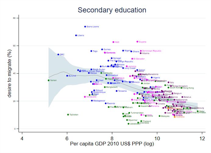
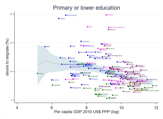
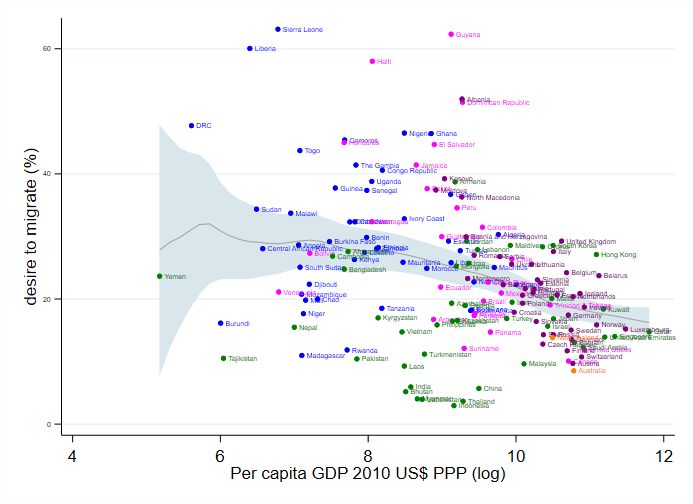
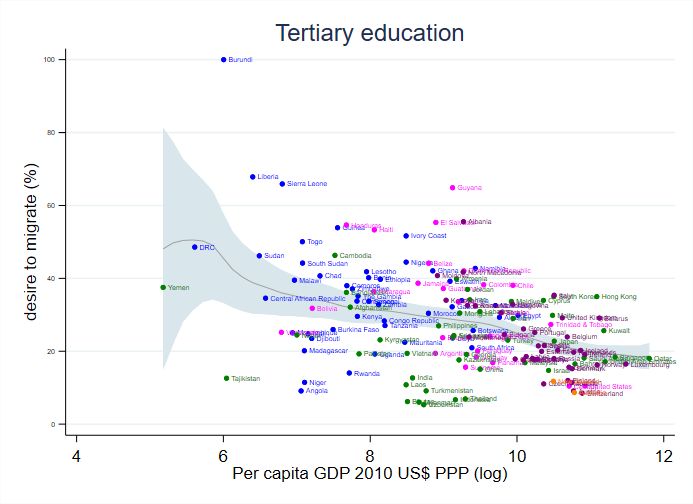
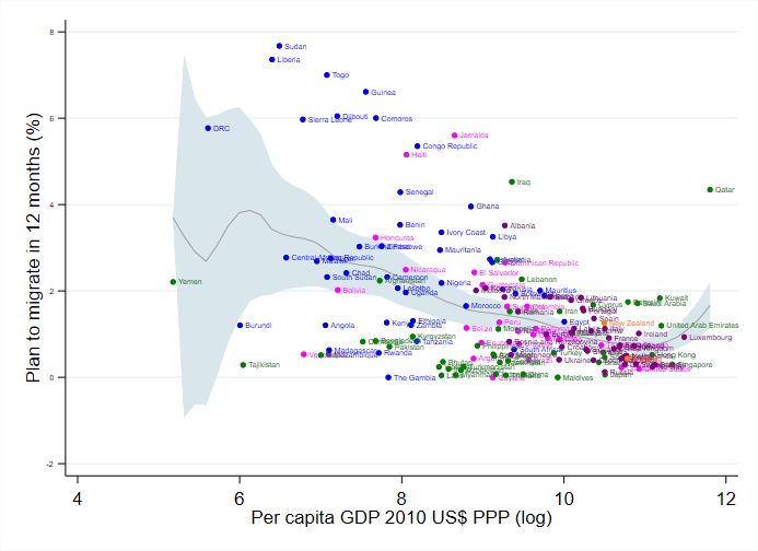
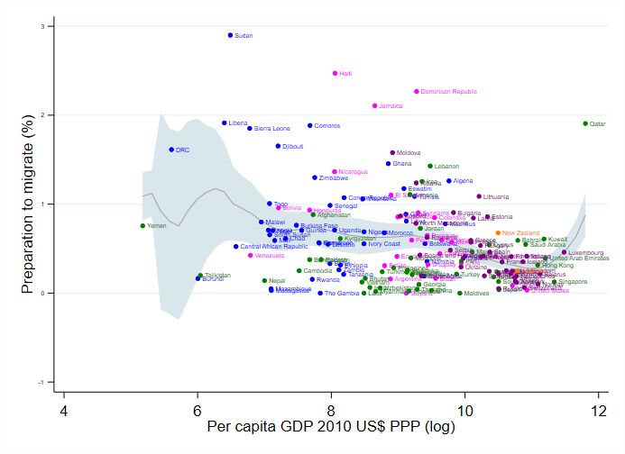
3. The desire to migrate

In this section we analyse the desire to migrate using model (2). We take a two-step
approach. In the first step we use the following specification for the utility from remaining in
the origin country:
 = 1 + (5)
where ot is an origin country-time fixed effect and estimate a logit model for the desire to
migrate. In this step, we estimate the impact of individual characteristics on the desire to
migrate. The country of origin characteristics will be subsumed within the fixed effect, the
estimate of which can be interpreted as the logs odds of wanting to move for someone with
the individual characteristics all equal to zero which we will refer to as the base
characteristics. In the second step we regress the estimated country-year fixed effects on
country-year variables.

Our primary interest is to investigate how income shapes the desire to migrate with a
particular focus on Zelinsky’s (1971) hypothesis of a hump-shaped relation between income
and migration. This hypothesis is usually expressed as a relationship at the country level but,
with our data, we can also investigate the impact of individual income18.

Figure 8 plots the share of people who want to migrate from the country against GDP per
capita. There is a lot of heterogeneity across countries; the desire to migrate varies from 3%
in Indonesia to 63% in Sierra Leone. From this graph, there seems to be a weak but negative,
almost linear, relation between GDP in the country of origin and the desire to emigrate, in
contrast to the Zelinsky’s hypothesis but in line with what Benček and Schneideheinze (2020)
find using panel data. Dao et al (2018) argue the relationship varies by education so Figure
B3 in the Appendix shows the correlation between demand for emigration and GDP per
capita by education level. The relationship seems to be negative for all education groups, with
similar monotonicity. Clemens and Mendola (2020) argue that it is the GWP questions that
ask about plans and preparation to emigrate that are more informative about likely migration
given real-world constraints; Figure B4 presents the relationship between the responses to
these questions and GDP per capita; Zelinsky’s hypothesis does not emerge strongly from
these figures. However, these relationships do not control for other relevant factors, so we
now turn to the estimates.

First-Step Estimates

Table 5 presents the results for the first step. Here, the key variable we are interested in is
annual equivalised household income, measured in 2010 dollars. Income and household size
are available in GWP only since 2009, so for this part of the analysis we have to discard years
between 2006 and 2008. In column 1 we present the results for a very simple model where
we include country-year fixed effects and income only, in a logarithmic form. In this
specification, we find that, within a given country-year, people from richer households are
significantly more likely to want to emigrate. Zelinsky’s hypothesis predicts a non-monotonic
relationship at the aggregate level, which may suggest that a similar functional form could
apply to the individual relation too. To test whether that is the case, column 2 adds a squared
term for the log of income, centred at $8,000, which is a value in the range of what is often

18
 Dustmann and Okatenko (2014) do something similar but study a question that includes the desire to migrate
internally and a measure of income “based on data on household assets (household ownership of durable
consumer goods and housing quality), and questions referring to sufficiency of current income” because, for
their years, actual household income was not available. Clemens and Mendola (2020) estimate the income
elasticity of emigration at the household level, with a focus on predicted actual migration in developing
countries rather than potential migration. They find the elasticity to be positive in their setting.

 13

argued in the literature to be the peak of the hump-shaped relation (see Benček and
Schneideheinze, 2020, for a review of the literature). When this functional form is
considered, the level becomes non-significant, while the square term is negative, implying
that the desire to migrate is non-monotonic peaking at $8,000. These estimates are in line
with the Zelinsky’s hypothesis at individual level.

The specification without any regressors other than income can be thought of as closest to the
way in which the Zelinsky’s hypothesis is normally described. However, as emphasized in
the introduction, development has many dimensions with different effects on the desire to
emigrate and it is important to understand these. Though this paper is primarily about the
impact of income, it is important to control for other relevant factors. In columns 3 and 4 we
re-estimate the models of columns 1 and 2 but now adding additional covariates; dummy
variables indicating the level of education, whether born abroad, gender, a set of dummy
variables for age, household size, number of kids under 15 in the household. The
characteristics are scaled so that the country-year fixed effect can be interpreted as desire to
migrate for a man, born in the country, aged 45 to 64 with primary or lower education, non-
married, in a household of 4, with 2 kids below the age of 15 living in the same household
and with equivalised household annual income of $8,000. In line with previous studies, we
find that the young, the more educated, and foreign born are more likely to want to migrate.
People who are married and who have a larger number of kids in the households are less
likely to want to move away. The coefficient on log household income is insignificantly
different from zero when only a linear term is included (column 3). The addition of a
quadratic term in column 4 has a significantly negative quadratic term but also a significantly
negative linear term meaning that the desire to migrate is decreasing at a household income
of $8,000. The estimates in column 4 imply a hump-shaped relationship in line with the
Zelinsky’s hypothesis but now peaking at an income of $1,800 i.e. much lower, meaning that
most of the sample is in the region where the desire to migrate is a decreasing function of
household income19. The change in the estimated impact of household income is largely
because of the role of education which is highly correlated with income. The estimates
suggest that those with higher levels of education are more likely to want to emigrate; this is
an important channel by which economic development may increase and not decrease the
desire to emigrate.

We next investigate whether the impact of household income varies with the average level of
income in a country as it is possible that relative income shapes the desire to migrate. The
effect of the average level of income itself will be subsumed within the fixed effects but we
can estimate the interaction between household and country-level income. A convenient way
to do this is to include the square in the deviation of household income from the country level
average income i.e. the following version of model (5):

 = 1 log + 2 (log ⁄8000)2 + 3 (log ⁄ ̅ )2 + + (6)

where is the per capita household income, and ̅ is the average per capita household income
in a given country and year. The results of this specification are reported in column 5. The
additional term is significant with a positive sign. One feature of the estimates in column 5 is that
the two squared terms appear to have virtually identical coefficients of different sign which
means the squared terms in household income would cancel out leaving only an interaction
between household income and country average income. This model is estimated in column

19
 The median for the household income per capita in our sample is approximately $2,800.

 14

6. The linear and interaction terms are significant20. The estimates imply that higher
household income is associated with an increased demand to emigrate for countries where
average household income is below approximately $2,20021 - but decreasing above that
point. The standard error of this estimate (computed using the delta method) is $819. The
finding that the relationship between household income and the desire to emigrate is
mediated by the level of aggregate income is in line with Clemens and Mendola (2020).

Income may not be the only aspect of the quality of life that affects the desire to emigrate. In
column 7 we add the measures of current and expected (in 5 years) life satisfaction, and a
variable that measures the individual satisfaction with the freedom in the country of origin (a
detailed description of the GWP questions is in Appendix A.2). Higher life satisfaction and
satisfaction with freedom are significantly associated with a lower desire to emigrate. The
inclusion of these variables the estimated impact of income. The estimates in column 7 now
imply that higher household income is associated with an increased demand to emigrate for
countries where the average income is below $8,400 – with a standard error of $4,510 - a
much higher turning point than in the estimates of column 6, though less precisely estimated
because the interaction term (which becomes the denominator when computing the turning
point) is small relative to its standard error.

There might be heterogeneity in the impacts, so columns 1 to 3 of Table B4 in the Appendix
estimates the model by education group. People with primary and secondary education have a
similar impact of income, and similar to the one estimated for the overall sample. But for
those with tertiary education there is very little relation between income and the desire to
emigrate.

Columns 4 and 5 of Table B4 in the Appendix report estimates of the same models replacing
the migration desire question with the migration planning and preparation questions. Column
4 estimates the model for the migration planning question i.e. those who report “planning to
move permanently to another country in the next 12 months”. Column 5 estimates the model
for those who report taking active preparation for a move. In both cases the results are
obtained conditioning on the structure of the questionnaire – i.e. the planning question is only
asked to people who desire to migrate, while the preparation question only to people who are
planning to migrate. In both cases the role of income has the same direction as in the model
for the responses to the migration desire question but the coefficient on the interaction term
not significantly different from zero making the impact of income positive for all sensible
values of average income in the country, consistent with Clemens and Mendola (2020). This
suggests that conditional on desiring to migrate, richer people in all countries tend to take
more ‘factual’ actions towards migration. This could be because they are more likely to have
the resources needed to turn a desire to migrate into action, but also because they are likely to
have more options to migrate to their desired destination.

Columns 6 and 7 of Table B4 take a different approach analysing unconditional responses to
the plan and preparation questions i.e. including those who report no desire to emigrate as
‘zeroes’. The results for planning to move illustrate also in this case a non-monotonic relation
with household income, the effect of household income is positive up until $26,000 and
20
 We also estimated a model including both (log ⁄8000)2 and the interaction term. The coefficient related to
the squared term is not significant in any of the relevant specifications, so we present only specifications with
the level of income and the interaction with average income.
21
 The turning point – here and in the following paragraphs - is calculated before applying the approximations
used in the tables we have in the paper, so calculations from the Tables displayed in this paper may not directly
give the exact turning point estimate to the reader.

 15

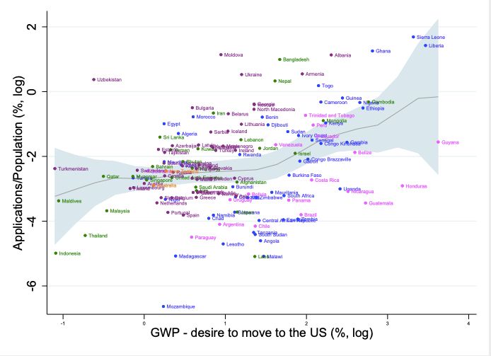
negative after that point but has a standard error of $36,218 so is not meaningful. For
preparation question the estimated relation is positive for any plausible range for the country
average household income.

Overall, the first-step estimates suggest a complicated relationship between measures of
welfare at the individual level and the desire to migrate. Higher education always seems to
be associated with a higher desire to migrate, but higher life satisfaction both currently and
expected in the future reduces the desire to emigrate. Higher household income has a positive
effect in poorer countries and a negative effect in richer countries. Though it should be noted
that the impact of income on the desire to migrate is always much smaller than the estimated
impact of destination country income in the desired destination models.

Second-Step Estimates

However, all these estimates include country-year fixed effects and we now move to the
second step, the analysis of these. We use the fixed effects estimated from the model of
column 6 of Table 5. These fixed effects can be interpreted as the log odds of wanting to
emigrate relative to wanting to stay for someone with the base characteristics in Table 5. We
regress the country-year fixed effects on a variety of origin-country level variables. In line
with (2) we also include the inclusive value from the desired destination model (computed
using our preferred specification for the destination model, column 4 of Table 3)22. The
inclusive value can be interpreted as a measure of how attractive the available destinations
are to a migrant from the source country. It would be therefore expected to be positively
related to the desire to migrate. For example, given that we find that destination country
income has a big effect on the desired destination and that people are less likely to want to
move to more distant countries, the inclusive value will be higher for migrants in source
countries that are closer to high-income countries.

Column 1 of Table 6 includes only the log of origin country GDP per capita and time effects.
There is a significant negative coefficient implying that those in richer countries are less
likely to want to emigrate. However, this specification cannot investigate the Zelinsky
‘hump-shape’ hypothesis that implies a non-monotonic relationship. To investigate this, we
include a linear spline in log GDP per capita with a knot at $8,00023; this specification is
reported in column 2. Now we find a significant negative relationship for the higher income
countries and an insignificant relationship for poorer countries.

Column 3 of Table 6 adds a range of other origin country variables, for instance population
and some push factors as the deaths from conflicts, the proportion of people affected by
natural disasters and a measure of the institutions in the country. We also include the
inclusive value, a measure of the utility from migrating from a given destination estimated by
our destination model. The impact of origin country income is similar in nature to that
reported in Column 2. The inclusive value has the expected positive sign, implying that those
in countries with closer connections to attractive destinations are more likely to want to
emigrate. The coefficient on the inclusive value can be usefully interpreted in the following
way. Imagine that the log income in all possible destination countries rises 0.1 i.e. a 10
percent rise. Because log income has a coefficient of 1.57 in column (4) of Table 3, this
would raise the inclusive value by 0.157. The coefficient on the inclusive value of 0.42 in

22
 This can be estimated most simply as the fixed effect in the Poisson regression model for desired destination.
23
 We prefer a linear spline to a quadratic as a quadratic forces a symmetry around the turning point that may not
be appropriate.

 16