Improving flood damage assessments in data-scarce areas by retrieval of building characteristics through UAV image segmentation and machine ...
←
→
Page content transcription
If your browser does not render page correctly, please read the page content below
Nat. Hazards Earth Syst. Sci., 21, 3199–3218, 2021
https://doi.org/10.5194/nhess-21-3199-2021
© Author(s) 2021. This work is distributed under
the Creative Commons Attribution 4.0 License.

Improving flood damage assessments in data-scarce areas by
retrieval of building characteristics through UAV image
segmentation and machine learning – a case study
of the 2019 floods in southern Malawi
Lucas Wouters1,2 , Anaïs Couasnon1 , Marleen C. de Ruiter1 , Marc J. C. van den Homberg2 , Aklilu Teklesadik2 , and
Hans de Moel1
1 Institutefor Environmental studies (IVM), Vrije Universiteit Amsterdam, De Boelelaan 1087,
1081 HV Amsterdam, the Netherlands
2 510, an initiative of the Netherlands Red Cross, Anna van Saksenlaan 50, 2593 HT Den Haag, the Netherlands

Correspondence: Lucas Wouters (wouters.lucas@outlook.com)

Received: 17 December 2020 – Discussion started: 15 January 2021
Revised: 11 September 2021 – Accepted: 14 September 2021 – Published: 27 October 2021

Abstract. Reliable information on building stock and its vul-     tainty in the derived damage curves is larger than in the haz-
nerability is important for understanding societal exposure       ard or exposure data. This research highlights the potential
to floods. Unfortunately, developing countries have less ac-      for detailed and local damage assessments using UAV im-
cess to and availability of this information. Therefore, calcu-   agery to determine exposure and vulnerability in flood dam-
lations for flood damage assessments have to use the scarce       age and risk assessments in data-poor regions.
information available, often aggregated on a national or dis-
trict level. This study aims to improve current assessments of
flood damage by extracting individual building characteris-
tics and estimate damage based on the buildings’ vulnerabil-      1   Introduction
ity. We carry out an object-based image analysis (OBIA) of
high-resolution (11 cm ground sample distance) unmanned           Worldwide, flooding is one of the most common and damag-
aerial vehicle (UAV) imagery to outline building footprints.      ing natural hazards in both monetary terms and loss of life
We then use a support vector machine learning algorithm           (UNDRR, 2019). Estimating flood damage is essential for
to classify the delineated buildings. We combine this in-         shaping flood risk management before and disaster response
formation with local depth–damage curves to estimate the          after a flood. This can be done a priori to support strategic
economic damage for three villages affected by the 2019           risk reduction by, for example, increasing awareness in areas
January river floods in the southern Shire Basin in Malawi        that are high in potential damage to therefore reduce vulner-
and compare this to a conventional, pixel-based approach          ability or after a given flood event to quickly derive estimates
using aggregated land use to denote exposure. The flood           of building damage to help with recovery and prioritize ac-
extent is obtained from satellite imagery (Sentinel-1) and        tions. This latter one is known as a damage and needs assess-
corresponding water depths determined by combining this           ment (DNA), which is usually based for the most part on data
with elevation data. The results show that OBIA results in        collected on the ground. For DNAs, household field surveys
building footprints much closer to OpenStreetMap data, in         are conducted as rapid DNAs and post disaster and needs as-
which the pixel-based approach tends to overestimate. Cor-        sessments (Jones, 2010). A priori flood damage assessments
respondingly, the estimated total damage from the OBIA is         are generally modeled and require extensive datasets on flood
lower (EUR 10 140) compared to the pixel-based approach           hazard characteristics, the exposed elements at risk and the
(EUR 15 782). A sensitivity analysis illustrates that uncer-      vulnerability of these elements (Budiyono et al., 2015; Alam,

Published by Copernicus Publications on behalf of the European Geosciences Union.
3200                                            L. Wouters et al.: Improving flood damage assessments in data-scarce areas

A. et al., 2018; UNDRR, 2019). Much work has focused on            data were used to derive exposure and vulnerability infor-
improving these damage estimates, quantifying the effect of        mation after which it was combined with available building
different flood scenarios and the consequences (Murnane et         information. The model was able to assess damage estimates
al., 2017; Jongman et al., 2012; de Moel et al., 2015). Unfor-     in an urban setting, with the total average damage deviating
tunately, sufficient information on the exposure and vulnera-      from the refund claims with a percentage error lower than
bility is often lacking or less accessible in developing coun-     2 %. Nonetheless, the authors state that a generalization of
tries (van den Homberg and Susha, 2018). Therefore, cal-           the procedure needs to be studied further. Another exam-
culations for flood damage assessments must use the scarce         ple of using indicator-based approaches regarding physical
data available, often aggregated on a high national or dis-        vulnerability, specifically tailored for data-scarce regions, is
trict level. This lack of data complicates accurate and down-      given by Malgwi et al. (2020). In this study, a conceptual
scaled flood damage assessments, as shown in studies by            framework is proposed that combines vulnerability indexes
Amirebrahimi et al. (2016) and Fekete (2012). The lower            and regional damage grades (frequently observed damage
spatial level is, however, required for most flood risk man-       patterns) by utilizing a synthetic “what-if” assessment by ex-
agement applications. Especially building damage remains           perts.
hard to quantify as existing classification categories often ne-      Remote sensing has the potential to generate information
glect spatial heterogeneity. This causes many uncertainties        on the exposure and vulnerability input for damage assess-
in the assessment about physical structure, content and flood      ments. Numerous studies have been carried out for mapping
susceptibility (Wagenaar et al., 2016). Flood damage assess-       land cover, such as built-up areas, with varying methods and
ments are a standard procedure to identify potential eco-          spatial scales (Mallupattu and Sreenivasula Reddy, 2013; Ai
nomic losses in flood-prone areas. With growing populations        et al., 2020). With new innovations in the resolution of im-
and economies, the need to accurately estimate flood dam-          agery, also smaller-scale studies can be conducted where re-
age is gaining greater importance (Merz et al., 2010). Such        mote sensing can be applied to retrieve information at the
assessments can enable the allocation of resources for re-         object level (Klemas, 2015; Englhardt et al., 2019). In a re-
covery and reconstruction by humanitarian decision-makers          view by De Ruiter et al. (2017) it is stated that common
when a disaster does strike (Díaz-Delgado and Gaytán Inies-        flood vulnerability studies that use land-cover types could be
tra, 2014). For example, severe floods in January 2015 have        improved by incorporating object-based approaches, for ex-
demonstrated the need for improved flood damage assess-            ample by developing vulnerability curves for different wall-
ments in Malawi. During this period, the worst flood disas-        material types. A technique to derive useful information from
ter in terms of economic damage was recorded for 15 of its         remotely sensed image data is object-based image analysis
28 districts, predominantly in the Southern Region. The to-        (OBIA). OBIA has the potential to identify exposed elements
tal damage was estimated to be USD 286.3 million, with the         and their characteristics accurately when incorporated into a
housing sector accounting for almost half of the total damage      flood damage assessment, but there is little literature com-
at USD 136.4 million (Government of Malawi, 2015). More            bining the methods. The process involves grouping pixels
recently, the Chikwawa District was subjected to extensive         into objects based on their spectral properties or external
flooding because of continuous rainfall by Tropical Cyclone        variables, after which they are combined into spatial units
Desmond in January 2019.                                           for image analysis such as image classification (Blaschke,
   Several studies have suggested that flood damage assess-        2010). Spectral properties to group these objects could, for
ments could be improved by incorporating the vulnerability         example, be the mean value or standard deviation of spectral
in building structures. Blanco-Vogt et al. (2015) summarize        bands of the image. A conventional workflow to conduct an
different methods to retrieve building characteristics and es-     OBIA consists of two major steps: (1) segmentation and (2)
timate flood vulnerability based on building types in a semi-      feature extraction and classification. The literature demon-
urban environment. Different building parameters are dis-          strates that the relationship between the objects under consid-
cussed that could affect the building susceptibility to flood-     eration and the spatial resolution is critical for the accuracy
ing, including height, size, form, roof structure, and the topo-   of segmentation and the OBIA, improving with the emer-
logical relation to neighboring buildings and open space.          gence of higher-resolution imagery (Blaschke, 2010; Belgiu
Types are created by taking the remotely sensed data and re-       and Draguţ, 2014; Xu et al., 2019).
lating this to potential flood impact. Blanco-Vogt et al. (2015)      In this research, automated object recognition and clas-
note that these types can be used to link buildings to more        sification from high-resolution images, based on an OBIA
detailed damage curves and discuss the challenges in terms         workflow, are used to delineate and characterize buildings in
of data resolution and techniques in remote sensing. The           a flood damage assessment. This object-based approach is
research of De Angeli et al. (2016) builds on the method           applied to the 2019 January flood event for three villages in
of Blanco-Vogt et al. (2015) by developing a flood damage          the Lower Shire Basin in Malawi and compared to a con-
model that differentiates the urban area (using building clus-     ventional flood damage assessment based on disaggregated
ters based on building taxonomies and footprints) instead of       census data and homogenous land-use pixels (pixel-based ap-
using a single homogenous land-use class. Remotely sensed          proach). By doing so, this study aims to

Nat. Hazards Earth Syst. Sci., 21, 3199–3218, 2021                                https://doi.org/10.5194/nhess-21-3199-2021
L. Wouters et al.: Improving flood damage assessments in data-scarce areas                                                 3201

    – create a framework to incorporate OBIA in flood dam-         responsible policy towards this type of event. One of the
      age assessments,                                             lessons learned from this event was that the lack of disag-
                                                                   gregated (spatial) data and information management slowed
    – assess the added value of high-resolution unmanned           down the disaster response and could eventually slow down
      aerial vehicle (UAV) imagery in creating object-level        recovery efforts as well (Government of Malawi, 2015).
      exposure and vulnerability data,                                Between 22 and 26 January 2019, the Chikwawa District
                                                                   was again subjected to extensive flooding because of contin-
    – compare flood damage estimates between an object-            uous rainfall from Tropical Cyclone Desmond. There is no
      based and conventional pixel-based approach.                 specific empirical damage data available for our case study
   In the next chapters we will introduce the case study area      area. However, the International Federation of Red Cross and
and the data, methods and results related to the pixel-based       Red Crescent Societies (IFRC) issued an Emergency Plan of
and object-based approach. In addition, a sensitivity analysis     Action (EPoA) after the floods. Based on preliminary assess-
is performed to illustrate which components of the risk as-        ment carried out by staff members and volunteers from the
sessment are most important when it comes to uncertainty in        Village Civil Protection Committee (VCPC) and Malawi Red
damage estimates.                                                  Cross Society (MRCS), one of the most affected areas is the
                                                                   Traditional Authority of Makhuwira with a total of 2434 col-
                                                                   lapsed houses (IFRC, 2019). In Chikwawa, a total of 15 974
2    Study area                                                    people were affected, 3154 houses damaged or destroyed,
                                                                   and 5078 people reported to be displaced across at least seven
Malawi is a landlocked country in sub-Saharan Africa, bor-         camps set up by communities and government. Most of the
dered by Zambia to the northwest, Tanzania to the northeast,       affected houses were semi-permanent buildings, which are
and Mozambique to the east, south and west. The country            also common in our study area (IFRC, 2019).
is vulnerable to a range of natural hazards including tropical
storms, earthquakes, droughts and floods. Especially floods
affect many sectors from agriculture to sanitation, environ-       3     Materials
ment, and education. A major contributing factor to this risk
is the variable and erratic rainfall, which often causes flood-    In order to determine the hazard, exposure and vulnerabil-
ing in lower-lying areas after falling in the highlands. Be-       ity for both the pixel- and object-based approaches, a variety
tween 1946 and 2013, floods accounted for 48 % of the major        of data sources have been used. This section describes these
disasters in Malawi. With a large rural population mostly re-      data sources, including remote sensing and other geospatial
lying on agriculture, these disasters have a large impact on       data (including UAV imagery), local survey, regional build-
the national economy and food security of the population           ing statistics, and the datasets used for the construction of
(Government of Malawi, 2015).                                      (local) damage curves.
   The southern Chikwawa District is one of the poorest and
most flood-prone in the country. In addition to being ex-          3.1    Remote sensing data
posed to flooding frequently, the district is characterized by a
largely rural population and home to highly vulnerable com-        UAV imagery was collected in November 2018 by The
munities in terms of economic diversification, employment          Netherlands Red Cross (NLRC) and the MRCS for mapping
opportunities and access to social services (Trogrlić et al.,     and flood simulation purposes in the Lower Shire Basin. A
2017). The Shire River is the largest river in the country         fixed-wing UAV (SmartPlanes Freya) with 0.3 m2 wing area,
and starts from lake Malawi flowing towards Chikwawa and           weighing around 1.5 kg, and with a RICOH GR II camera
into the low-lying Mozambique plain, as shown in Fig. 1. In        was used to obtain the UAV imagery. The drone usually flew
the district of Chikwawa, our study area, the river meets a        around 300 m altitude, having a flight time of around 60 min
large flood plain called the Elephant Marsh. This floodplain       per battery and with a sidelap and overlap of each 70 %.
is characterized by stagnant flows, with the marsh varying in      The flights were carried out without ground control points
size depending on the flow of the river. When rainfall is high,    (GCPs). Van den Homberg et al. (2020) give a detailed de-
large areas may be underwater.                                     scription of the UAV model and data collection. Agisoft Pho-
   In 2015, Malawi underwent some of the worst flooding            toScan and Metashape software was used to stitch the images
ever recorded in the country, affecting 1 101 364 people, dis-     of the optical imagery and extract a digital surface model
placing 230 000, and killing 106. In the aftermath, it be-         (DSM) from the stereophotogrammetry. The extent of the
came clear that the housing sector accounted for most of           flight coverage is shown in Fig. 1.
the total damage with almost 40 % followed by agriculture             In addition to UAV imagery, other remote sensing data
with approximately 20 %. The worst affected districts were         were acquired from open-source databases, including the
in the Southern Region, being the districts of Chikwawa and        Shuttle Radar Topography Mission (SRTM) digital elevation
Nsanje, and the disaster sparked a discussion about a more         model (DEM) collected by NASA and the synthetic aper-

https://doi.org/10.5194/nhess-21-3199-2021                                 Nat. Hazards Earth Syst. Sci., 21, 3199–3218, 2021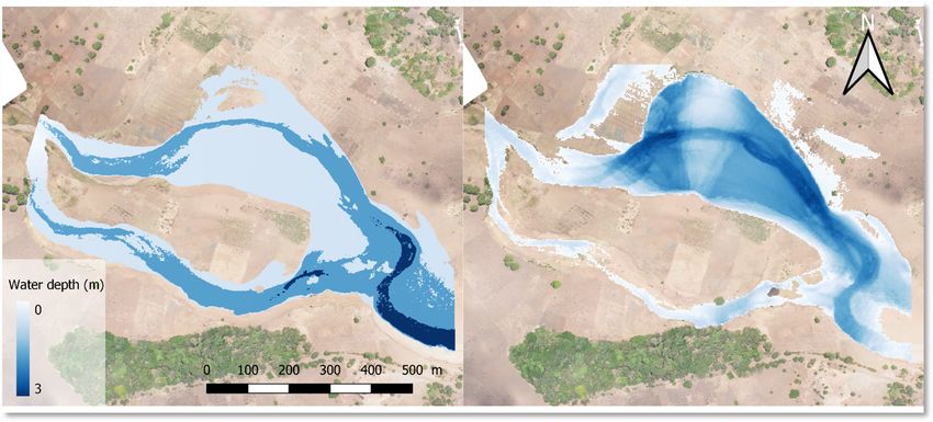
3202 L. Wouters et al.: Improving flood damage assessments in data-scarce areas
Figure 1. The geographical location of Malawi (left) and the District of Chikwawa (right). © Google Maps, 2021.
ture radar (SAR) Sentinel-1 imagery collected by Copernicus collected characteristics of potential flood vulnerability pa-
(Farr and Kobrick, 2000). The High-Resolution Settlement rameters, including size, height, roof material, wall material
Layer (HRSL) provides an estimate of the settlement extent and inventory of the house. These parameters were selected
and population density and was developed by the Connec- based on key features that characterize building types in the
tivity Lab at Facebook in combination with the Centre for region along with their spectral differences, making them
International Earth Science Information Network (CIESIN) easier to detect from remote imagery.
by using computer vision techniques to qualify optical satel- In addition to the local field survey data, building stock
lite data with a resolution of 0.5 m (CIESIN, 2016). The used in the pixel-based approach was extracted from the In-
OpenStreetMap (OSM) contains a features layer of manu- tegrated Household Survey 2016–2017 (IHS4), conducted by
ally delineated objects and was used for validation purposes the Malawi National Statistical Office (NSO) (Malawi Statis-
(© OpenStreetMap contributors, 2019). Table 1 summarizes tical Office, 2017). This report describes the distribution of
the various datasets. three main building types by aggregating data to a regional
level. A distinction is made based on their building material:
3.2 Building data
– A permanent building has a roof made of iron sheets,
tiles, concrete or asbestos, and walls made of burned
To gain information about the building stock present in the
bricks, concrete or stones.
case study area, Teule et al. (2019) conducted a field sur-
vey in four villages in, or surrounding, the Traditional Au- – A semi-permanent building is a mix of permanent and
thority Makhuwira (including Jana, Nyambala and Nyangu). traditional building materials and lacks the construction
The data were collected by randomly selecting buildings in materials of a permanent building for walls or the roof.
the vicinity of these interviews. In total, 50 buildings were That is, it is built of non-permanent walls such as sun-
sampled and assumed to be representative buildings in es- dried bricks or non-permanent roofing materials such
timating the different building characteristics present in the as thatch. Such a description would apply to a building
area. The OSM data layer reports on a total of around 1350 made of red bricks and cement mortar but roofed with
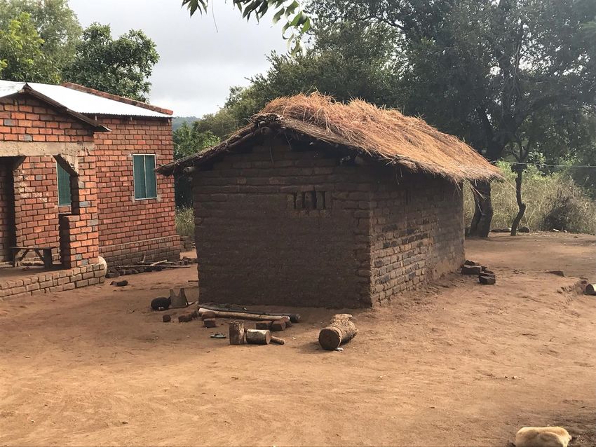
buildings in the villages selected for our analysis. Figure 2 grass thatching.
shows an example of one the sample buildings. The survey
Nat. Hazards Earth Syst. Sci., 21, 3199–3218, 2021 https://doi.org/10.5194/nhess-21-3199-2021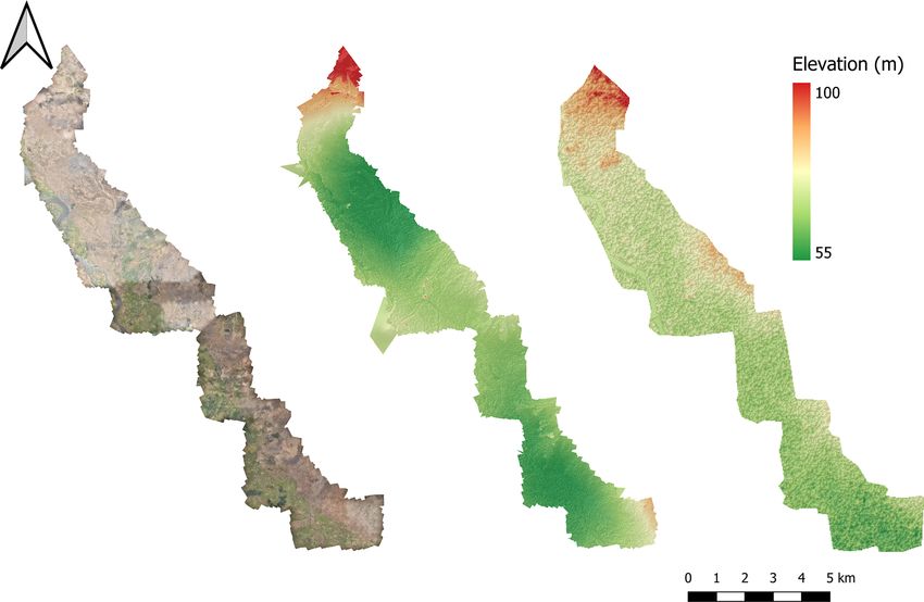
L. Wouters et al.: Improving flood damage assessments in data-scarce areas 3203
Table 1. Available datasets in this research. Abbreviations: digital elevation model (DEM), digital surface model (DSM), ground range
detected (GRD), Malawi Red Cross Society (MRCS), OpenStreetMap (OSM) and Shuttle Radar Topography Mission (SRTM) synthetic
aperture radar (SAR).
Datasets and Type Resolution Data repository Acquisition Used for
platforms (horizontal)
Remote sensing
Space shuttle DEM 30 m SRTM, Earth Explorer Unknown Flood hazard
Satellite SAR 23 m Sentinel-1 (GRD), Copernicus 24 Jan 2019 Flood hazard
UAV Optical 0.11 m MRCS Nov 2018 Exposure & vulnerability (object-based)
UAV DSM 0.25 m MRCS Nov 2018 Exposure & vulnerability (object-based)
Geospatial
HRSL Land cover 30 m CIESIN 2016 Exposure (pixel-based)
OSM Vector Object OpenStreetMap n/a OBIA validation
The term n/a stands for not applicable.
3.3 Damage curve data
Stage-dependent damage curves are created for different
building types by extracting material-specific vulnerability
functions from the CAPRA (probabilistic risk assessment)
platform. This platform contains a library with pre-defined
analytical vulnerability functions, including different con-
struction materials, calibrated with expert-supplied parame-
ters (CAPRA, 2012). These curves express relative damage
as a percentage with respect to water depth. Several exam-
ples in the library include concrete, wood, reed, masonry and
earth (unfired) materials.
In addition to the vulnerability curves, maximum building
damage values were estimated based on the different kinds of
materials and the costs of buildings found in southern Malawi
(Table 5). The values were validated by local authorities in
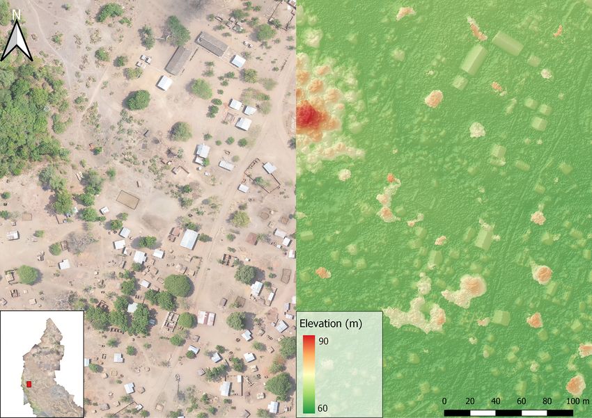
Figure 2. Image from one of the sample buildings taken in the the case study area during interviews by Teule et al. (2019).
case study area taken by T. Teule (23 June 2019). A clear con-
trast between building material is visible between the two buildings:
thatched roofs and unburned brick walls (middle building) versus 4 Methods
iron sheeted roofs and burned brick walls (left building).
This section describes the two flood damage assess-
ment methods compared: first, the conventional pixel-based
– A traditional building is made from traditional method and second the proposed object-based method, after
housing construction materials such as mud walls, which their distinctive components are discussed in more de-
grass/thatching for roofs and rough poles for roof tail.
beams.
4.1 Flood damage assessment
The ratio of the different dwellings in the district of Chik-
wawa is summarized in Table 2. From this information, a Figure 3 presents the workflow applied in this study to de-
trend can be observed towards a ratio with more formal build- rive the flood damage estimates from the January 2019 flood
ings. The most recent statistics – being the building stock event in the case study area. Following the general procedure
information from 2016 to 2017 – is used in the pixel-based of a flood damage assessment, both approaches can be di-
flood damage assessment. vided into three separate components: hazard, exposure and
vulnerability (Merz et al., 2010; de Moel and Aerts, 2011;
Jongman et al., 2012); see Fig. 3. In this research, we de-
fine the hazard as the flood extent and depth of a flood event,
https://doi.org/10.5194/nhess-21-3199-2021 Nat. Hazards Earth Syst. Sci., 21, 3199–3218, 2021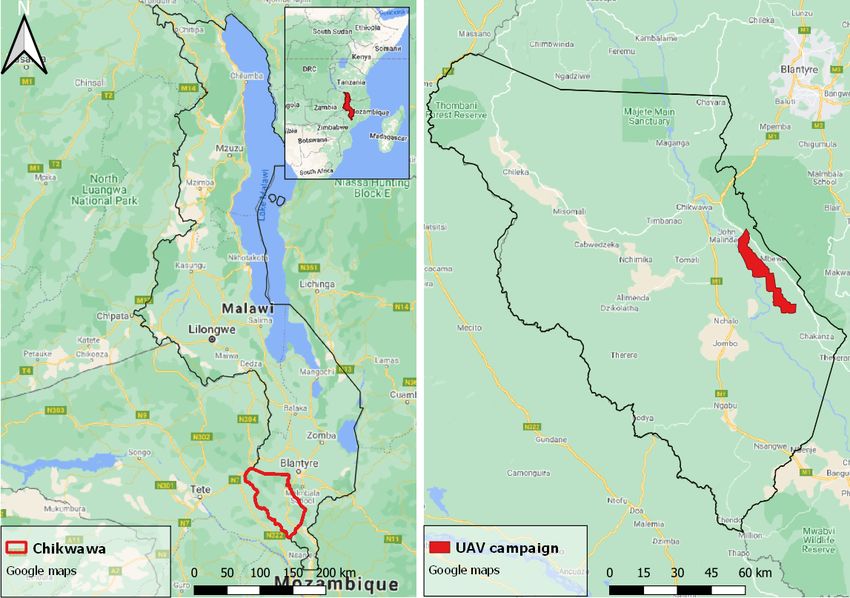
3204 L. Wouters et al.: Improving flood damage assessments in data-scarce areas
Table 2. Ratios of building stock in the Chikwawa District of southern Malawi (Malawi Statistical Office, 2017).
Permanent (%) Semi-permanent (%) Traditional (%)
Building stock 2010–2012 25.5 15 59.5
Building stock 2016–2017 33.7 33.8 32.5
exposure as the exposed buildings to this flood, and vulnera- metric correction using the terrain correction function. Water
bility as the susceptibility of these buildings to flooding. and non-water are separated through setting a threshold by
For the pixel-based approach, the HRSL land-use map, analyzing the backscatter coefficient histogram and manu-
containing homogenous land-use pixels, is used to determine ally determining the peak characteristics of land and water
the built-up area. Building stock information from Table 2 areas. Flooded areas could then be determined by setting a
is used to create corresponding stage-damage curves for the threshold value of 0.0022 which was defined based on the
defined building types (Malawi Statistical Office, 2017). histogram plot of pixel values for reflectivity.
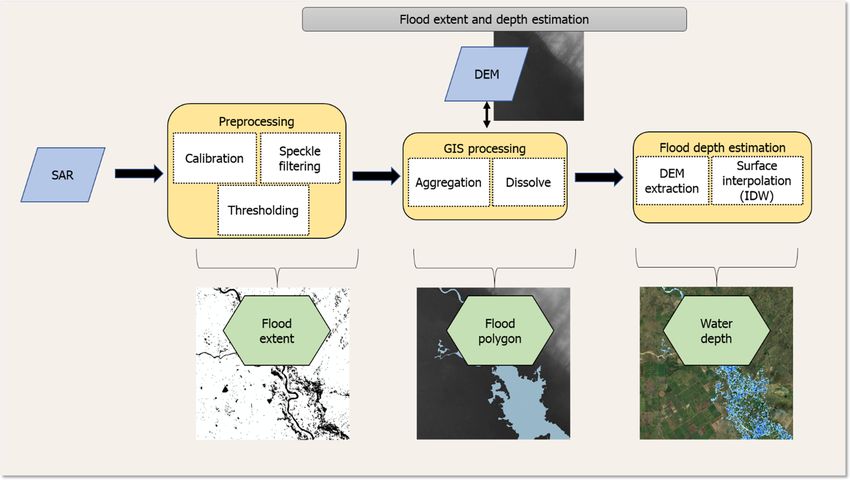
For the object-based assessment, we combine informa- The flood raster map was further prepared in ArcGIS by
tion from an OBIA of high-resolution UAV imagery with vectoring the resulting water pixels using the “raster to vec-
the stage-damage curves created from the field observations. tor” tool and aggregating with the “aggregate polygons” tool
Building footprints are detected and classified based on their based on a neighborhood of 100 m. Single-pixel polygons
aerial features to identify local building types. Local stage- were removed to exclude noise from the flood map, and any
damage curves are then assigned to these types by assessing empty spaces in the polygon were filled using the “union”
the vulnerability of buildings found in the field survey. and “dissolve” tools. These filled spaces can be the result of
Both flood damage assessments are inherently different on beneath-vegetation flood areas that can be missed by the SAR
the classification of exposed elements and their flood sus- processing (Shen et al., 2019). Negative values are removed
ceptibility. In the terminology of the UNDRR (2019), this in the next, final step if they are a result of actual topographic
translates into different input data for the exposure and vul- factors, such as local hills.
nerability components. The final step in this approach follows the research of Cian
The two different approaches share the same hazard com- et al. (2018) and Cohen et al. (2018), in which the flood
ponent, being the 2019 flood event. Based on Sentinel-1 boundaries along the water surface are used to estimate the
satellite imagery, a flood extent is created, and its related wa- elevation of the water surface. The boundaries of the derived
ter depth is estimated. The economic damage is calculated by flood extent were turned into points with the “raster to point”
combining the flood impact with the different sets of expo- tool, after which the elevation values were extracted from the
sure data and damage curves (Fig. 3). In order to determine DEM. The water surface was then computed using the “in-
the relative influence of the different components on the re- verse distance weighting” (IDW) tool. Essentially, this means
sulting risk, we evaluate the influence of building size, water that pixels inside of the flood extent get the elevation value
depth and damage curve on our damage assessment model of the closest elevation points along the boundary. The water
using a one-at-a-time sensitivity analysis, as applied in Ke et depth can then be calculated by deducting the initial DEM
al. (2012). values from the assigned water surface values. Figure 4 visu-
alizes the workflow and the resulting output.
4.2 Hazard: flood area and water depth estimation To validate the surface water interpolation method, the re-
sult is compared with a flood hazard map obtained from a
hydraulic 1D steady model that was run for a subsection of
To represent the flood hazard, we derive water depths from
the Shire River (Maparera River) in a study by Copier et
the January 2019 flood event using the workflow presented
al. (2019). The segment covers an area of 2.1 km2 in which
in Fig. 4. This approach takes the following three main steps:
the river has a total length of 2.2 km. The model was run
(1) extracting SAR data and processing them using SNAP
using Hydrologic Engineering Center’s River Analysis Sys-
software (SNAP, 2019) to create a flood extent map, (2)
tem (HEC-RAS) software (Hydrologic Engineering Center,
preparation of the data in ArcGIS, and (3) using the avail-
1998). Due to a lack of historical data, the discharge val-
able SRTM DEM to estimate the water surface elevation and
ues used as input for the model are estimated to match the
extracting the flood water depth.
case study area’s water flowing abilities without creating an
Extracting and processing SAR data was based on the
extreme overflow. The discharge value was set to 50 m3 s−1 ,
SNAP flood mapping workflow (McVittie, 2019). This in-
and the Manning coefficient was set to 0.05. For both the sur-
volved preprocessing of the SAR imagery through calibra-
face water interpolation method and the hydraulic model run,
tion to transform the pixels from the digital values recorded
the UAV DSM is used as input.
by the satellite into backscatter coefficients, speckle filter-
ing using the “Lee filter” to remove thermal noise and geo-
Nat. Hazards Earth Syst. Sci., 21, 3199–3218, 2021 https://doi.org/10.5194/nhess-21-3199-2021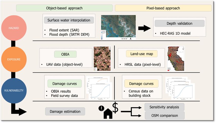
L. Wouters et al.: Improving flood damage assessments in data-scarce areas                                                         3205

Figure 3. Workflow of the two approaches of flood damage estimation. The left panel shows the object-based approach, and the right panel
shows the pixel-based approach. Abbreviations: synthetic aperture radar (SAR), Shuttle Radar Topography Mission (SRTM) digital elevation
model (DEM), object-based image analysis (OBIA), High-Resolution Settlement Layer (HRSL) and OpenStreetMap (OSM). The inundation
(hazard) map is shown on a © Google Satellite image. The OBIA and land-use maps are created using UAV imagery from the Malawi Red
Cross Society.

Figure 4. The workflow representing the extraction of SAR satellite imagery and deriving its corresponding water depth. The flood polygon
is shown on a SRTM DEM image, and the water depth map is shown on a © Google Satellite image.

   The root mean square error (RMSE) is used to evaluate               operating characteristic (ROC) curve. The ROC curve is a
the output from both approaches (Cohen et al., 2018). By               probability curve and reports the true positivity rate (TPR),
doing so, it can be determined to what extent the output of            also called recall (R), as a function of the false positive rate
both approaches deviate in terms of water depth estimation.            (FPR). The area under curve (AUC) represents the degree or
In addition to the root mean, we also construct the receiver           measure of separability, with 1 representing a model with a

https://doi.org/10.5194/nhess-21-3199-2021                                    Nat. Hazards Earth Syst. Sci., 21, 3199–3218, 2021
3206                                           L. Wouters et al.: Improving flood damage assessments in data-scarce areas

perfect predictability, 0 with complete unpredictability and
0.5 with random guesses. The HEC-RAS flood map is taken
as ground truth against the results of the surface water inter-
polation method, in which a prediction can be either a true
positive (TP), false positive (FP), true negative (TN) or false
negative (FN). The TPR and the FPR are calculated as fol-
lows:
        TP
TPR =         ,                                            (1)
      TP + FN
         FP
FPR =         .                                            (2)
      TN + FP
4.3     Exposure

4.3.1    Pixel-based approach

For the pixel-based approach, the built-up area is estimated      Figure 5. Steps of the OBIA: (a) original UAV imagery, (b) result
by taking the built-up area of the pixel according to average     of mean shift segmentation and (c) classification using SVM classi-
density percentages and building sizes. This density is deter-    fier. The image contains UAV imagery collected by the Malawi Red
mined by visual interpretation of the UAV imagery. The per-       Cross Society (MRCS), collected in November 2018. Made with
centages found in the distribution of building types reported     QGIS.
by the IHS4 are used to calculate the damage corresponding
to 1 pixel unit.

4.3.2    Object-based approach                                       After the segmented objects were classified, a filtering pro-
                                                                  cess was conducted in which objects were removed based
The OBIA consisted of the following steps (Fig. 6). First,        on their respective height and category. By keeping the two
validation and training samples were collected from the vil-      categories that represent buildings with a height over 0.5 m,
lages in the case study area by manually delineating objects.     buildings can be extracted, and potential misses are excluded
We manually delineated a total of 144 building to serve as        from the damage calculation. This height was chosen as a
training and 556 as validation. This step was followed by seg-    value between the height of the ground and a one-story build-
menting the high-resolution imagery and classifying the vec-      ing. The mean height from the DSM was added to the objects
torized objects. We selected the open-source geo-software         by creating centric points of each segment and extracting the
Orfeo ToolBox (OTB). This toolbox is a library for image          elevation values to these points from the UAV DSM map. To
processing initiated by the CNES (French Space Agency)            derive the height of these objects, a baseline DEM was con-
that includes numerous algorithms created for the purpose         structed and subtracted from the mean DSM value. For this,
of segmentation and classification (Grizonnet et al., 2017).      the cells classified as “metal” and “thatch” were removed
   Segmentation was performed using the mean shift clus-          from the DEM. Next, ground reference points were placed
tering algorithm utilized by OTB. The mean shift algorithm        using visual interpretation to make sure no bushes or trees
exploited by Orfeo relates to the work of Michel et al. (2015),   were selected. The elevation of these ground reference points
in which the goal of image segmentation is to partition large     was correspondingly used to interpolate an elevation surface
images into semantically meaningful regions. The following        using IDW, and the elevation of this interpolated surface was
parameters were set: (1) the spatial radius or the neighbor-      used to determine the height of the metal and thatch cells by
hood distance was set to 1.5 m, (2) the range is expressed in     determining the difference with the original DEM elevation.
radiometry units in the multispectral space to 5 m, and (3) the      To evaluate the performance of the OBIA model, a map
minimum size of a segmented region was set to 5 m2 in rela-       with 556 manually delineated and labeled reference build-
tion to minimum building sizes. The support vector machine        ings was compared to a map with predicted buildings from
(SVM) algorithm from the same Orfeo library served to clas-       the classification. For this purpose, a confusion matrix was
sify the vectorized objects from the segmentation. The SVM        created (Gutierrez et al., 2020), in which TP is the number
is a kernel-based machine learning algorithm that has been        of cases detected both manually and with the automatic ap-
effectively used to classify remotely sensed data (Mountrakis     proach. FP is the number of cases detected by the automatic
et al., 2011). The classifier was trained on samples that rep-    approach but not manually. TN is the number of cases de-
resented the common features in the selected images and are       tected manually but not by the automatic approach. FN is the
summarized in Table 3. An example of the output of this pro-      number of undetected cases. The statistical parameters that
cess is shown in Fig. 5.                                          were used to test the classification performance are the accu-

Nat. Hazards Earth Syst. Sci., 21, 3199–3218, 2021                                https://doi.org/10.5194/nhess-21-3199-2021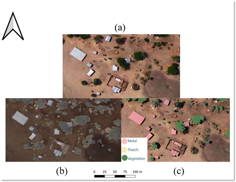
L. Wouters et al.: Improving flood damage assessments in data-scarce areas                                                        3207

Figure 6. Conceptual model of the building classification using automatic extraction methods.

Table 3. Samples used as input for training the SVM classifier with mean value ranges of the spectral bands (nm).

                                  Value    Label          Samples     Mean B0     Mean B1       Mean B2
                                  1        Vegetation           28    121–164      135–165      101–136
                                  2        Metal                27    207–241      207–244      205–245
                                  3        Thatch               31    225–241      201–228      184–213
                                  4        Bare ground          34    171–220      155–197      145–197
                                  5        Shadow               24    113–154      114–150      113–137

racy and F1-score. The overall accuracy (A) was calculated              where θ ∧ is the predicted value, θ i is the value of the refer-
given Eq. (1).                                                          ence buildings, and N is the sample size.
          TP + TN
A=                                                             (3)      4.4   Vulnerability: damage curve estimation
     TP + FP + TN + FN
To test the classification performance per class, the F1-score          Corresponding to the building types found in the exposure
was used. This statistic is the weighted mean of both preci-            component of each flood damage assessment, a set of dam-
sion (P ) and R, where 0 indicated the lowest possible score            age curves is created. The description of the different types
and 1 a perfect score. The parameters are calculated with the           and their construction material is used to weigh material-
following equations:                                                    specific damage curves from the CAPRA library, according
       TP                                                               to the method proposed by Rudari et al. (2016). We make use
P=           ,                                                 (4)      of the expanded aggregation table as proposed by Rudari et
     TP + FP
                 P ·R                                                   al. (2016), including the construction material considered for
F1-score = 2 ·        .                                        (5)      every building type (Table 4). This table indicates for each
                 P +R
                                                                        building type the building stock material for which CAPRA
To evaluate the building area, predicted buildings were cho-            damage curves are used.
sen that have partial or complete overlap with the reference               For the pixel-based approach, three curves are created for
buildings. From this selection, the relative error (RE) was             each of the building types (traditional, semi-permanent, per-
calculated per building type. In this case, the absolute error          manent), making use of the description of wall building ma-
is normalized by dividing it by the magnitude of the value              terials in the fourth Integrated Household Survey 2016–2017
of the reference buildings. The RE is calculated through the            (IHS4). Next, the distribution of these three building types
following expression:                                                   (Table 2) is used as weights to create a single curve that can
       PN                                                               be applied to the urban pixels from the land-use map. For in-
               θ∧ − θi                                                  stance, semi-permanent housing consists of unburned bricks,
RE = n=1  PN           ,                                   (6)
             i=1 |θ i|
                                                                        for which the masonry and earth CAPRA curves should be

https://doi.org/10.5194/nhess-21-3199-2021                                     Nat. Hazards Earth Syst. Sci., 21, 3199–3218, 2021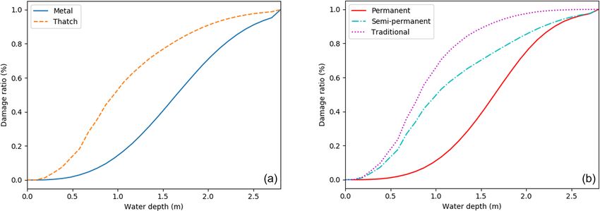
3208                                                L. Wouters et al.: Improving flood damage assessments in data-scarce areas

Table 4. Aggregation table of the CAPRA damage curves based on building stock information.

                 CAPRA materials            Building stock material                                  Building types
      Concrete    Masonry    Earth   Wood                             Metal roof    Thatch roof      Permanent    Semi-permanent    Traditional
                       ×                    Burned bricks                 ×             ×                ×
                       ×      ×             Unburned bricks                             ×                                ×
      ×                                     Concrete                                                     ×
                              ×             Mud                                         ×                                                 ×
                                      ×     Wood                                        ×                                                 ×

used. In this case, these curves are averaged and used to rep-             Table 5. Estimated maximum damage values per square meter
resent a semi-permanent building.                                          based on local knowledge of replacement costs (Teule et al., 2019).
   For the object-based approach, the results from the field
survey are used to create damage curves for building types                                    Type                    EUR m−2
determined by aerial observation and the OBIA (metal roof                                     Permanent                  15.20
and thatch roof). The materials of the roofs are correlated                                   Semi-permanent             10.60
with wall material, based on the field observations from                                      Traditional                 4.40
which we derive the wall-to-roof relationships. The local dis-                                Metal roof                 13.00
tribution found in wall material is used to weigh the curves                                  Thatch roof                 9.70
from the CAPRA library based on percentages. This means,
for example, that the distribution in wall material found for
buildings with a thatch roof – being burned bricks, unburned                  – a(ip ) is the size of the building in area (m2 ).
bricks, mud and wood – are used to weigh the CAPRA
curves. These materials correspond to the masonry, masonry                    – r(i) is the ratio of the type according to the national
and earth, and earth and wood CAPRA curves, respectively.                       survey in Table 2.
   In both approaches, we follow Maiti (2007) and assume                      – rc(i) is the replacement cost per square meter based on
that buildings constructed with a mud wall tend to collapse                     the type (i); see Table 5.
at a water depth of 1 m. Before creating curves for each build-
ing type, this damage curve from the CAPRA library (earth                  For the object-based approach, damage is calculated per ob-
curve) is modified so that 1 m of inundation corresponds to a              ject by combining buildings automatically detected and clas-
100 % damage value.                                                        sified through OBIA with the local stage-damage curves cre-
                                                                           ated from the field survey. The damage can be calculated
4.5       Risk: damage estimation                                          through the following expression:
                                                                                            2
For the pixel-based approach, the built-up area is estimated                                X
by taking the built-up area of the pixel according to average              Do [EUR] =             damage (io ) · a(io ) · rc(io )[EUR],           (8)
                                                                                            i=1
density percentages and building sizes. The average density
percentages and building sizes will be collected by visual in-             where the variables are as follows:
terpretation of the UAV imagery. The percentages found in
                                                                              – io is the building type based on the roof type and wall-
the distribution of building types reported by the IHS4 are
                                                                                to-roof relationships (i.e. metal roof and thatch roof).
used to calculate the damage corresponding to 1 pixel unit.
The damage is calculated through the following expression:                    – damage(io ) is the damage per building in euros calcu-
                                                                                lated with the local stage-damage curve and using as
                 3
Dp [EUR] =
                 X
                       damage ip ·a ip ·r ip ·rc ip [EUR], (7)                  input the flood water depth (m) for this building.
                 i=1
                                                                           4.6     Sensitivity analysis
where the variables are as follows:
  – ip is the building type (i.e. traditional, semi-permanent,             To quantify how the damage parameters can influence the
    permanent) as determined by the building stock descrip-                damage estimate, a one-at-a-time sensitivity analysis will be
    tion of the Malawi National Statistical Office (2017).                 conducted by increasing and decreasing the different damage
                                                                           parameters with the mean of the respective relative errors.
  – damage(ip ) is the damage per pixel in euros calculated                The sensitivity value (SV) will be used to represent the sen-
    with the adjusted stage-damage curve and using as input                sitivity and can be calculated by dividing the largest resulting
    the water depth (m) in the considered pixel.                           damage by the smallest resulting damage (Koks et al., 2015).

Nat. Hazards Earth Syst. Sci., 21, 3199–3218, 2021                                           https://doi.org/10.5194/nhess-21-3199-2021
L. Wouters et al.: Improving flood damage assessments in data-scarce areas 3209
5 Results 5.3 Damage curves and maximum damage values
5.1 UAV imagery Figure 9 shows the two damage curves created for the object-
based approach based on types corresponding to the field sur-
Figure 7 shows the resulting UAV-based orthophoto, includ- vey (left) and three for the types in the building stock descrip-
ing the DSM with shaded relief and the SRTM DEM with tion of IHS4 national survey that are used in the pixel-based
shaded relief, from the flight area. The Shire River is cap- approach (right). Metal-roofed buildings show a lower vul-
tured at the western side of the acquired imagery. Complet- nerability than thatch-roofed at the same water depth due to
ing the area took 140 flights, each lasting around 45 min. The the structural integrity accompanied by more formal build-
UAV-based DSM shows a relatively equal elevation through- ing material. Similar patterns can be observed for the damage
out most of the area. However, the absence of GCPs influ- curves based on the description of building stock in the Chik-
enced the global accuracy of the elevation. A deviation can wawa District. Similar to how the damage curves were de-
be observed when we compare the UAV-based DSM to the rived, maximum damage values have also been determined.
SRTM DEM. This DEM shows a down-sloping pattern of The damage values per square meter for all building types
the elevation towards the south, in accordance with the flow can be found in Table 5.
of the Shire River.
Although this difference hampers large-scale (hydraulic) 5.4 OBIA quality assessment
analysis using the UAV-based DSM, it is still valuable in as-
sessing the local height variation of objects on a microscale. The implementation of the OBIA model had a varying degree
Figure 8 gives a detailed overview of the town of Chagambat- of success according to the statistical tests. Table 6 shows
uka, including the UAV-based DSM. Buildings can clearly be that classification is more reliable for classifiers that have a
distinguished based on their rectangular shape and elevation, clear spectral difference with surrounding elements, such as
while trees are generally the tallest objects in the area. shadow and metal roofs, whereas bare ground and thatched
roofs are less easy to distinguish. This spectral difference re-
5.2 Field observations
sulted in a higher F1-score for buildings with a metal roof
Based on the information collected through the building sur- (89 %) compared to those with a thatched roof (53 %). With
vey, buildings in the case study area are grouped into two the F1-score being the harmonic mean of the precision and
types based on their distinctive aerial features. From the 50 recall, this metric captures both the false negatives and the
samples, no buildings were found that have a wall structuring false positives of the classification process. The lower F1-
resembling wood, reed or concrete. In addition, no buildings score for detected thatch roofs could be attributed to their
were found having tiles or any other material as the roof, nor tendency to blend in with the environment because of their
any having more than two levels. relatively similar spectral properties. With the addition of
The first type of building in the area is composed of burned the height threshold for objects, the individual F1-scores for
and, in a small number of cases, unburned bricks. This type buildings were improved to 90 % for metal-roofed buildings
is less vulnerable to flooding compared to the other type due and 72 % for thatch-roofed buildings. The increased F1-score
to its material being less susceptibility to building failure. Its for thatch-roofed buildings indicates that having additional
main distinctive aerial feature is a metal sheet roof, but the and accurate information on the height of the objects has
results of the OBIA and the field survey also indicate that a large effect on the individual classification accuracy. The
this type of building has a larger footprint than thatch-roofed overall accuracy of the initial run shows a value of 77.45 %,
buildings. For the metal-roofed buildings, two wall materials indicating the amount of correctly classified objects out of
were found: burned red bricks (90 %) and unburned bricks the total amount of samples. This value also increases up
(10 %). to 80 % with the addition of a height threshold for objects,
The second type is generally composed of less formal though this increase is also partly due to the exclusion of
building material, with its main distinctive feature being a poorly performing classes such as “bare ground”.
thatch roof. The results of the survey seem to indicate a rel- The building objects from the OBIA are a direct result
atively equal distribution between the building materials, but of the segmentation process, and the relative error seems to
as unburned bricks and mud walls are more susceptible to reflect the same pattern as the classification process. This
building failure, this type is considered more vulnerable to means that buildings with a thatch roof tend to be harder
flooding. For the thatch-roofed buildings, three wall materi- to detect because the model groups pixels together that rep-
als were found: burned red bricks (27 %), unburned bricks resent different objects, such as bare ground and the thatch
(41 %) and mud/wattle (32 %). roof. For both types, the relative error between observed and
predicted building areas can be observed in Fig. 10. For the
thatch-roofed buildings, 50 % of the predictions are found
with RE lower than 30 %. For the metal-roofed buildings,
this same percentage of predictions are found with a RE
https://doi.org/10.5194/nhess-21-3199-2021 Nat. Hazards Earth Syst. Sci., 21, 3199–3218, 20213210 L. Wouters et al.: Improving flood damage assessments in data-scarce areas Figure 7. Example of the orthophoto (left) and DSM (middle) with shaded relief, produced with images from the UAV flight, and a Shuttle Radar Topography Mission DEM (right) with shaded relief. Made in QGIS using UAV imagery collected by the Malawi Red Cross Society (MRCS). Figure 8. Section of the town of Chagambatuka in the northern part of the UAV campaign area, with orthophoto (left) and DSM with shaded relief (right) produced with images from the UAV flight. Made in QGIS using UAV imagery collected by the Malawi Red Cross Society (MRCS). Nat. Hazards Earth Syst. Sci., 21, 3199–3218, 2021 https://doi.org/10.5194/nhess-21-3199-2021
L. Wouters et al.: Improving flood damage assessments in data-scarce areas 3211
Figure 9. Constructed damage curves for the two types derived from field and aerial observations for the object-based approach (a), and
three types derived from the description of building stock at district level for the pixel-based approach (b) (Malawi National Statistical
Office, 2017). The water depth is the flood water relative to the ground floor.
Table 6. Evaluation of the performance accuracy of the OBIA classification.
Label F1-score F1-score∗ Accuracy (%) Accuracy (%)∗
Vegetation 0.91 – 77.45 80.19
Metal 0.89 0.90
Thatch 0.53 0.72
Bare ground 0.49 –
Shadow 0.90 –
∗ Addition of height threshold by subtracting the extracted DSM and DEM values.
lower than 7.5 %. Generally, metal-roofed buildings tend to
be larger in size than thatch-roofed buildings, with a mean
building size of 39 and 21 m2 , respectively. For both types,
the RE tends to decrease as building size increases. This
seems to be in line with the literature in which it is stated
that if objects get closer to the size of the available spatial
resolution, errors are more likely to occur (Blaschke, 2010).
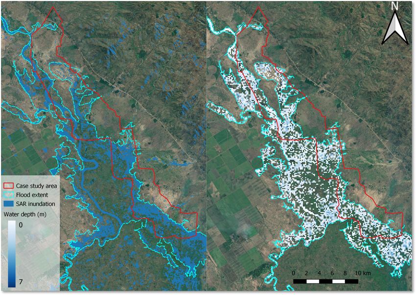
5.5 Flood inundation
To check whether the surface interpolation method ad-
equately captures flood characteristics, we compare our
method with the results from a hydrodynamic model applied
at the Maparera River. Figure 11 shows the maximum water
depth obtained from both methods. The average water depth
from the flood event at the Maparera River was 1.17 m for
the surface water interpolation and 1.22 m for the hydraulic
model run using the UAV DSM (Copier et al., 2019). The
maximum estimated water depth for both approaches was
Figure 10. Building area and relative error for both types (metal and about 3 m (3.30 and 2.79 m, respectively). The RMSE was
thatch) in the case study area. calculated to be 0.73 m. The results show that for a flood
depth of approximately 3 m, the surface water interpolation
method deviated from the hydraulic model by < 0.75 m on
average. We found considerable differences between both
https://doi.org/10.5194/nhess-21-3199-2021 Nat. Hazards Earth Syst. Sci., 21, 3199–3218, 20213212 L. Wouters et al.: Improving flood damage assessments in data-scarce areas
models along the main channel. This is in line with research 5.7 Sensitivity analysis
from Cohen et al. (2018) given the inability of similar meth-
ods to calculate complex fluid dynamic effects. In addition, By varying the building size and water depth parameters with
the interpolation method shows relatively low water depth the mean of the respective relative errors, the sensitivity of
at the upstream boundary compared to the hydraulic model. the damage parameters for both approaches was estimated.
Nevertheless, the interpolation model seems to correctly dis- As there is no information on the uncertainty of the dam-
solve the higher-elevation area between the two main chan- age curve values from the CAPRA database, the influence of
nels from the aggregated flood extent that was extracted from this parameter is derived by using only the lowest and high-
Sentinel-1 imagery. The AUC measured 0.73 (see Fig. A1), est damage curves from the building types. For example, the
indicating an acceptable agreement between the HEC-RAS lower damage bound for the damage curve sensitivity value
reference map and the water depth map resulting from sur- in the object-based approach is computed by using only the
face water interpolation (Hosmer and Lemeshow, 2000). metal-roofed damage curve and the higher bound using the
Repeating the method for the total case study area with the thatch-roofed damage curve. Table 7 shows that the largest
SRTM DEM produced a water depth map with an average variance in resulting damage is caused by this variance in the
water depth of 1.26 m and a maximum water depth of 7 m damage curves, meaning that the damage curve selection has
(see Fig. 12). Buildings in the inundated area were assigned the highest effect on the resulting damage estimates.
the water depth in the corresponding cell. Several areas with Similar results have been found by Saint-Geours et
a positive water depth can be observed in the resulting flood al. (2015) in a cost-benefit analysis of a flood mitigation
map that deviate from the SAR inundation map. These areas project in which the uncertainty in the depth–damage curves
indicate the subtraction of incorrect water depth values from is the prominent factor for estimating damage to private
the digital terrain model (DTM) or capture areas that were housing. Studies by de Moel et al. (2012) and Winter et
not identified with SAR imagery, for example, due to high al. (2019) also note that the most influential parameter in the
vegetation. uncertainty of flood damage estimates is the damage func-
tion. Moreover, it can be observed that the sensitivity value
of building size is lower in the object-based approach com-
5.6 Damage estimates pared to the pixel-based approach (1.21–1.43), which can be
attributed to less uncertainty in total building area that is
flooded. This indicates that, for the object-based approach,
By overlaying the separate components of the flood damage the increased accuracy with which buildings can be identified
assessment, the estimated damage was calculated for both leads to a decrease in the uncertainty of damage estimates.
approaches using Eqs. (7) and 8. Compared to the pixel- The water depth parameter reveals that, although uncertainty
based approach, the object-based approach provides a lower in water depth results in varying damage estimates, sensitiv-
estimation of the exposed built-up area of about two-thirds ity values for both approaches are comparable (1.46–1.56).
(Table 6). Interestingly, comparing the number of buildings Therefore, considering the same flood impact in each flood
in OSM, this comes very close to the amount extracted by the damage assessment does not affect damage estimates differ-
OBIA, giving confidence in the object-based approach. This ently.
amount of exposure influences the resulting damage con- It is apparent from Table 7 that all parameters involved
siderably. The flooded built-up area for the pixel-based ap- in the flood damage estimation include an amount of uncer-
proach and the object-based approach was estimated at 2541 tainty, and this propagates in the total estimated damage. As
and 3952 m2 , respectively. This resulted in estimated flood the flood map in both calculations remained equal, the differ-
damage of approximately EUR 10 000 and EUR 16 000, re- ences can be attributed to the sensitivity of the damage pa-
spectively (Table 6). rameters to the building types and damage curve parameters
Although building densities and average buildings sizes or the exposure and vulnerability components.
were extracted from the same UAV imagery, a difference can
be observed in the flooded built-up area between the two ap-
proaches. This is the result of the inability of land-use pixels 6 Discussion
to account for spatial variability in the building objects inside
a certain area. The preceding sections illustrate that by using OBIA, flood
Similar research on flood events in urban and rural areas damage can be estimated at the object level using UAV-
in Ethiopia, Germany and Poland exemplifies that significant derived imagery to detect buildings and classify them based
uncertainties are present in flood damage assessments due to on aerial features. This contributes to the literature in several
information lacking on the number of flooded buildings, the ways. Complementing a study by Englhardt et al. (2019),
building types considered in the assessment and the distri- which provides an impressive first glance at studies that
bution of building use within the flooded area (Merz et al., use object-based data to classify buildings into vulnerability
2004; Englhardt et al., 2019; Nowak Da Costa et al., 2021). classes, our approach enables us to use this information to
Nat. Hazards Earth Syst. Sci., 21, 3199–3218, 2021 https://doi.org/10.5194/nhess-21-3199-2021L. Wouters et al.: Improving flood damage assessments in data-scarce areas 3213 Figure 11. The estimated water depth from the HEC-RAS hydraulic model (left) and the derived water depth following the surface interpo- lation method (right) at the Maparera River. Made in QGIS using UAV imagery collected by the Malawi Red Cross Society (MRCS). Figure 12. The flood extent for the case study area extracted from SAR imagery (left) and the derived water depth map using surface water interpolation based on the SRTM DEM (right). The inundation maps are shown on © Google Satellite images. calculate damage at the individual building level. Therefore, ble if the scarcity of empirical loss data hinders the imple- our method provides more certainty on the number of flooded mentation of multivariate models, as is the case in most de- buildings, their size and location. A more recent study by veloping countries. Our study indicates, however, that OBIA Malgwi et al. (2021) suggests that using data-driven ap- combined with local data can accurately estimate flood dam- proaches, such as multivariate damage models, could further age in an area where such data are absent, for example, due improve estimates in data-scare regions compared to more to its remoteness. expert-based approaches. However, this is not always feasi- https://doi.org/10.5194/nhess-21-3199-2021 Nat. Hazards Earth Syst. Sci., 21, 3199–3218, 2021
You can also read