Box model trajectory studies of contrail formation using a particle-based cloud microphysics scheme
←
→
Page content transcription
If your browser does not render page correctly, please read the page content below
Research article
Atmos. Chem. Phys., 22, 823–845, 2022
https://doi.org/10.5194/acp-22-823-2022
© Author(s) 2022. This work is distributed under
the Creative Commons Attribution 4.0 License.

       Box model trajectory studies of contrail formation using
            a particle-based cloud microphysics scheme
                               Andreas Bier1 , Simon Unterstrasser1 , and Xavier Vancassel2
       1 Deutsches   Zentrum für Luft- und Raumfahrt, Insitut für Physik der Atmosphäre, Oberpfaffenhofen, Germany
                                  2 ONERA, The French Aerospace Lab, Palaiseau, France

                                    Correspondence: Andreas Bier (andreas.bier@dlr.de)

                                     Received: 29 April 2021 – Discussion started: 21 May 2021
                        Revised: 2 December 2021 – Accepted: 7 December 2021 – Published: 18 January 2022

      Abstract. We investigate the microphysics of contrail formation behind commercial aircraft by means of the
      particle-based LCM (Lagrangian Cloud Module) box model. We extend the original LCM to cover the basic
      pathway of contrail formation on soot particles being activated into liquid droplets that soon after freeze into
      ice crystals. In our particle-based microphysical approach, simulation particles are used to represent different
      particle types (soot, droplets, ice crystals) and properties (mass/radius, number). The box model is applied in
      two frameworks. In the classical framework, we prescribe the dilution along one average trajectory in a single
      box model run. In the second framework, we perform a large ensemble of box model runs using 25 000 different
      trajectories inside an expanding exhaust jet as simulated by the LES (large-eddy simulation) model FLUDILES.
         In the ensemble runs, we see a strong radial dependence of the temperature and relative humidity evolution.
      Droplet formation on soot particles happens first near the plume edge and a few tenths of a second later in the
      plume centre. Averaging over the ensemble runs, the number of formed droplets and ice crystals increases more
      smoothly over time than for the single box model run with the average dilution.
         Consistent with previous studies, contrail ice crystal number varies strongly with atmospheric parameters like
      temperature and relative humidity near the contrail formation threshold. Close to this threshold, the apparent ice
      number emission index (product of freezing fraction and soot number emission index) strongly depends on the
      geometric-mean dry core radius and the hygroscopicity parameter of soot particles. The freezing fraction of soot
      particles slightly decreases with increasing soot particle number, particularly for higher soot number emissions.
      This weakens the increase of the apparent ice number emission index with rising soot number emission index.
         Comparison with box model results of a recent contrail formation study by Lewellen (2020) (using similar
      microphysics) shows a later onset of our contrail formation due to a weaker prescribed plume dilution. If we
      use the same dilution data, our evolution and Lewellen’s evolution in contrail ice nucleation show an excellent
      agreement cross-verifying both microphysics implementations. This means that differences in contrail properties
      mainly result from different representations of the plume mixing and not from the microphysical modelling.
         Using an ensemble mean framework instead of a single trajectory does not necessarily lead to an improved sci-
      entific outcome. Contrail ice crystal numbers tend to be overestimated since the interaction between the different
      trajectories is not considered.
         The presented aerosol and microphysics scheme describing contrail formation is of intermediate complexity
      and thus suited to be incorporated in an LES model for 3D contrail formation studies explicitly simulating the
      jet expansion. Our box model results will help interpret the upcoming, more complex 3D results.

Published by Copernicus Publications on behalf of the European Geosciences Union.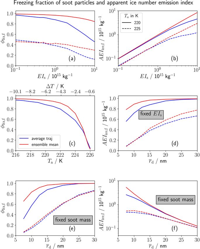
824                                                                             A. Bier et al.: Contrail formation trajectory studies

1   Introduction                                                       and chemical models, they have a simplified representation
                                                                       of microphysical processes. The main assumption in those
Aviation contributes to around 5 % of the anthropogenic cli-           3D studies is that contrail formation is triggered by hetero-
mate impact (Lee et al., 2021), where contrail cirrus is the           geneous ice nucleation on chemically activated soot particles
largest known contributor in terms of radiative forcing (e.g.          following Kärcher (1998). Chemical activation means that at
Boucher et al., 2013; Bock and Burkhardt, 2016). Due to pro-           least 10 % of the particle surface needs to be covered with
jections of large increases in air traffic, this contribution is ex-   sulfuric acid to form a thin liquid layer around the particle
pected to increase significantly (Bock and Burkhardt, 2019).           due to adsorption of water molecules. First, these studies as-
The number of nucleated contrail ice crystals has a large im-          sume plume water saturation to be sufficient for the activa-
pact on contrail cirrus properties and their life cycle (e.g. Un-      tion of soot particles, but the Kelvin effect requires, in par-
terstrasser and Gierens, 2010; Bier et al., 2017; Burkhardt et         ticular for soot particles with sizes of a few nanometres, that
al., 2018). The formation of contrails depends on complex              water saturation is clearly surpassed. This might cause a sig-
(thermo)dynamic, microphysical and chemical processes in               nificant overestimation of the number of formed ice crystals.
the exhaust plume, leading to a large variability in initial ice       Second, experimental investigations have shown that fresh
crystal numbers.                                                       engine soot particles are not supposed to be good ice nuclei
   Measurements and observations implicate that contrails              (e.g. Bond et al., 2013). This strengthens the requirement of
form once the plume mixture between the exhaust and ambi-              a transient liquid phase according to the SA criterion. Third,
ent air reaches or surpasses water saturation. This condition          aviation soot develops through incomplete combustion of hy-
is mathematically cast in form of the Schmidt–Appleman                 drocarbons (Bockhorn, 1994) and is mainly composed of el-
(SA) criterion, a relation derived purely from the thermody-           ementary carbon, causing a weak hygroscopicity. Laboratory
namics of the mixing process (Schumann, 1996).                         studies reveal the existence of active sites on soot particles,
   Plume exhaust particles, in particular soot but also ambi-          which develop by the attachment of functional groups and
ent particles entrained into the plume, can activate into wa-          enable the adsorption of water molecules (Popovicheva et
ter droplets and subsequently freeze to ice crystals by homo-          al., 2017). Since nitrate species and hydroxyls also have a
geneous nucleation (Kärcher et al., 2015). Ultrafine volatile          great potential to interact with soot particles (e.g. Kärcher
particles resulting from recombination of ion clusters and             et al., 1996; Grimonprez et al., 2018), the coating of soot
molecules (Yu and Turco, 1997) may also contribute to the              by sulfuric acid is not mandatory for their activation into
formation of ice crystals but typically require high (> 10 %)          water droplets. This fact explains why visible contrails can
water supersaturation to form water droplets due to their              still form when almost desulfurized fuel is burnt (Busen and
small size of a few nanometres (Kärcher and Yu, 2009). Con-            Schumann, 1995).
trail ice nucleation typically occurs within the first second of           Lewellen (2020) uses the more appropriate microphysical
plume mixing during the jet phase.                                     pathway consistent with the SA criterion and considers soot,
   Several studies on contrail formation in jet exhaust plumes         ambient and volatile particles as exhaust particle types po-
have been conducted in the past. At the moment, there are              tentially activating into water droplets and forming ice crys-
basically two complementary model approaches to study the              tals. However, these exhaust particles are assumed to have
contrail formation which either focus on jet dynamics or on            a monodisperse (or at best bidisperse) size distribution. This
plume microphysics. On the one hand, 0D box models based               does not sufficiently capture the Kelvin effect-related compe-
on a few idealized air parcel trajectories originating from an         tition among differently sized aerosol particles and possibly
engine (e.g. Kärcher and Yu, 2009; Wong and Miake-Lye,                 leads to ice crystal size spectra that are too narrow. In gen-
2010) are in general equipped with detailed microphysical              eral, Lewellen (2020) investigated the sensitivity of contrail
and chemical schemes. However, they neglect the large spa-             ice crystal numbers to properties of the different exhaust par-
tial variability in jet plumes arising from turbulent mixing of        ticles and to ambient conditions as well as engine configura-
the hot exhaust with ambient air and simulate only an aver-            tions, both within 3D LES and within a box model. Many
age mixing state over the whole plume cross-sectional area.            findings related to contrail formation rely on results from
Spatial inhomogeneities (in particular, strong radial gradi-           box models or analytical approaches with a crude representa-
ents and turbulent perturbations) in plume temperature and             tion of plume heterogeneity. By employing the same micro-
relative humidity are not considered. This leads to uncertain-         physics in 3D LES and in a box model with a mean dilution
ties in representing contrail ice crystal formation with un-           derived from the former model, Lewellen (2020) highlights
clear implications on contrail properties during the subse-            for which parameter configurations findings drawn from box
quent vortex and dispersion phase. On the other hand, sev-             model results are similar to those from 3D LES. Contrail ice
eral three-dimensional (3D) large-eddy simulations (LESs)              crystal numbers per burnt fuel mass are consistent in both
studying the contrail formation in the near-field plume (Paoli         model frameworks for low exhaust particle numbers or in
et al., 2013; Khou et al., 2015, 2017) resolve many details of         scenarios where ice crystals mainly form on ambient aerosol
the jet flow and account for spatial variation in the plume.           particles. However, the box model generally overestimates
Even though they are equipped with sophisticated aerosol               these ice crystal numbers for soot particle numbers of current

Atmos. Chem. Phys., 22, 823–845, 2022                                                    https://doi.org/10.5194/acp-22-823-2022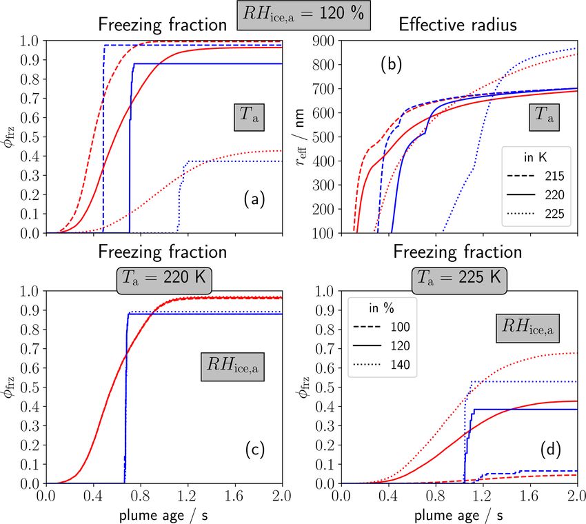
A. Bier et al.: Contrail formation trajectory studies                                                                          825

engines/fuels. Moreover, the ice crystal formation on emitted       microphysics and highlighted differences between the meth-
ultrafine volatile particles becomes more substantial in the        ods. The two studies have the following improvements com-
LES than in the box model.                                          pared to the online 3D studies of Khou et al. (2015, 2017):
   The basic objective of the project “ConForm” funded by           they include different types of aerosol particles, the chemi-
the Deutsche Forschungsgemeinschaft (DFG) is to combine             cal processing of fuel sulfur and the formation and growth
the advantages of the two complementary approaches, which           of volatile particles. Curvature and the solution effect are
means to simulate contrail formation in the expanding jet by        accounted for. A further improvement is prescribing log-
means of 3D LES with an improved representation of cloud            normally size-distributed soot particles using 60 size bins and
microphysics. For this, we will employ the LES model EU-            varying the geometric-mean dry core radius between 10 and
LAG (Smolarkiewicz and Grell, 1992), which is fully cou-            30 nm.
pled with the particle-based ice microphysics scheme LCM               For conventional aircraft engines, soot particles are in gen-
(Lagrangian Cloud Module; Sölch and Kärcher, 2010). The             eral the major source for the formation of contrail ice crystals
model system EULAG-LCM has been used for contrail sim-              (e.g. Kärcher et al., 1996; Kärcher and Yu, 2009; Kleine et
ulations during the vortex phase (e.g. Unterstrasser, 2014)         al., 2018). The number of emitted soot particles significantly
and the dispersion phase (e.g. Unterstrasser et al., 2017a, b).     influences the contrail cirrus climate impact (Burkhardt et al.,
This has been done with an EULAG version that does not              2018). Since engine soot emissions are quite variable and un-
yet support the compressible and gas dynamics equations.            certain, particularly in terms of their number and size (e.g.
Hence in a next step, LCM will be coupled to an up-to-date          Anderson et al., 1998; Petzold et al., 1999; Schumann et al.,
EULAG version that accounts for compressibility effects in          2002; Agarwal et al., 2019), our main focus is to investigate
the jet plume.                                                      the sensitivity of contrail properties (during their formation
   So far, LCM includes ice crystal formation as it occurs          stage) to different specific soot properties. We will also anal-
in natural cirrus clouds. The present paper describes how the       yse the variability of contrail ice nucleation with ambient
LCM model has been extended in order to cover the specifics         conditions as already explored by Bier and Burkhardt (2019)
of contrail formation and is a first step towards the goals of      using the analytical parameterization of Kärcher et al. (2015).
ConForm. Our main objective is to test the extended LCM in
a simple dynamical framework by running it in a box model           2     Methods
set-up. The microphysical parameterization is similar to that
in Lewellen (2020), but the numerical approach of the mi-           This section gives a short overview of the basic Lagrangian
crophysics differs as our study relies on a particle-based de-      Cloud Module (LCM) (Sect. 2.1), which has been exten-
scription and not on an Eulerian spectral bin model. More-          sively used for simulations of natural cirrus as well as
over, we prescribe soot particles by a log-normal instead of a      young and aged contrails in the recent past. Section 2.2
monodisperse or bidisperse size distribution.                       then describes in more detail the modifications and exten-
   Paoli et al. (2008) and Vancassel et al. (2014) extended the     sions for simulating contrail formation, and Sect. 2.3 gives an
box model framework to a multi-0D approach. Here, “multi-           overview about the general plume evolution and our trajec-
0D” means that the box model was run for a large ensemble           tory data. Finally, we will explain the box model framework
of trajectories that sample the expanding jet plume as pro-         in which LCM is employed in the present study.
vided by 3D LES and that represent many different plume
dilution developments. In such an “offline” approach, the mi-
                                                                    2.1    Particle-based LCM microphysics
crophysics can be more advanced than in a full 3D frame-
work with “online” microphysics. In our study, we intend to         The particle-based ice microphysics model LCM (Sölch and
highlight the importance of the huge variability in thermody-       Kärcher, 2010) comprises explicit aerosol and ice micro-
namic and contrail properties resulting from the variability        physics and is employed for the simulation of pure ice clouds
in the inhomogeneous turbulent mixed jet plume. Therefore,          like natural cirrus (e.g. Sölch and Kärcher, 2011) or con-
we will use an ensemble of many trajectories where the data         trails (e.g. Unterstrasser, 2014; Unterstrasser and Görsch,
have been taken from Vancassel et al. (2014). We expect that        2014; Unterstrasser et al., 2017a, b). In a particle-based mi-
the temporal evolution of ensemble mean properties leads to         crophysical approach, hydrometeors (like ice crystals or wa-
improved scientific results compared to those using one sin-        ter droplets) are described by simulation particles (SIPs) un-
gle average trajectory.                                             like traditional Eulerian approaches, where cloud properties
   Paoli et al. (2008) mainly studied the temporal evolution        are usually described by field variables. LCM has been used
of concentrations and (apparent) emission indices of volatile       in conjunction with the LES flow solver EULAG, which
particles and ice crystals depending on the fuel sulfur con-        computes the evolution of momentum, temperature and wa-
tent. Vancassel et al. (2014) revealed the spatial variability in   ter vapour. We omit the details about the coupling between
thermodynamic quantities and contrail properties. Moreover,         EULAG and LCM as in the present box model approach
they used an online method with less detailed contrail mi-          background temperature and water vapour concentration are
crophysics and an offline method with more detailed contrail        prescribed and not simulated. Each SIP represents a certain

https://doi.org/10.5194/acp-22-823-2022                                               Atmos. Chem. Phys., 22, 823–845, 2022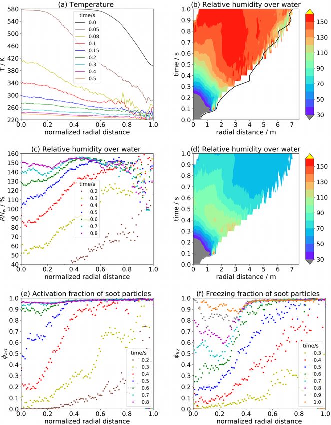
826 A. Bier et al.: Contrail formation trajectory studies
number νi of real ice crystals with identical properties and NSIP above around 100. Since this threshold value slightly
stores information about the single ice crystal mass mi , the varies with the geometric-mean dry core radius and particle
weighting factor νi and the ice crystal habit, among others. size distribution width, we choose a default value of around
Microphysical processes on the simulation particles include NSIP = 130.
homogeneous freezing of liquid super-cooled aerosol parti-
cles, heterogeneous ice nucleation, deposition growth of ice 2.2.2 Basic formation pathway
crystals, sedimentation, aggregation, latent heat release and
radiative impact on particle growth. For the contrail forma- In general, the moist exhaust plume cools due to mixing with
tion simulations, many of those processes (e.g. aggregation, ambient air. Contrails can form if ambient temperature is be-
sedimentation, radiation-related effects) are switched off. In low the so-called Schmidt–Appleman (SA) threshold tem-
the extended LCM, which will be described next, initial perature (2G ), and the plume becomes water-supersaturated
SIPs represent soot particles, which then become activated in a certain temperature range. The threshold temperature
into water droplets and eventually freeze (assuming suitable varies with atmospheric parameters (ambient relative humid-
background conditions). The SIP data structure is augmented ity over water, air pressure) and engine/fuel properties (spe-
and stores information about the particle type (soot, droplet, cific combustion heat, propulsion efficiency, water vapour
ice crystal) and properties (number, mass/radius, freezing emission index). The calculation of 2G is described in Ap-
temperature). pendix 2 of Schumann (1996).
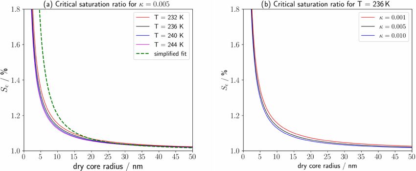
We use the Kappa–Köhler theory (Sect. 2.2.3) to calculate
which soot particles are able to activate into water droplets.
2.2 Microphysics of contrail formation Thereby, we prescribe the hygroscopicity parameter of soot
particles as a measure for their solubility. This is a more
2.2.1 Exhaust particles
convenient approach than defining a fixed fuel sulfur con-
In this study, we consider soot to be the only exhaust parti- tent since other polar species may lead to active sites on soot
cle since it plays a major role for contrail formation behind particles as well. Smaller soot particles require higher water
conventional passenger aircraft (e.g. Kärcher et al., 1996; supersaturation to overcome the Köhler barrier than larger
Kärcher and Yu, 2009; Kleine et al., 2018). Background par- ones (Fig. B1). Therefore, the latter particles can activate
ticles will become relevant for aircraft with soot-poor or earlier and may suppress the droplet formation on smaller
even soot-free emissions as for liquid hydrogen propulsion particles due to depletion of water vapour. The super-cooled
(Kärcher et al., 2015; Rojo et al., 2015). Even though ultra- droplets subsequently grow by condensation as long as the
fine volatile particles become more substantial for contrail exhaust air remains water-supersaturated. They freeze into
ice crystal formation in a 3D LES set-up (Lewellen, 2020), contrail ice crystals when the homogeneous freezing temper-
they are supposed to have a tiny impact on contrail formation ature (Sect. 2.2.5) is reached. Larger droplets can freeze ear-
for current soot-rich emissions in a box model framework lier (i. e., at higher plume temperature) and grow further by
(Kärcher and Yu, 2009). Hence, we neglect volatile particles deposition before smaller droplets manage to freeze into ice
in the present study, but we will incorporate this particle type crystals.
in the next model version.
The size spectrum of soot particles ranges from a few 2.2.3 Köhler theory
to hundreds of nanometres with geometric-mean values of
To calculate the equilibrium saturation ratio over a droplet
around 15 nm (Petzold et al., 1999). Soot particles are com-
or ice crystal surface (SK ), we use the Kappa–Köhler equa-
posed of several nanometre-sized primary spherules com-
tion (Petters and Kreidenweis, 2007):
bined into aggregates. For simplicity, we assume a spheri-
cal shape. Recent studies indicate a fractal irregular shape
Ke r 3 − rd 3
2 σ Mw
of the larger (more than several 10 nm) soot particles (e.g. SK = aw ·exp = 3 ·exp , (1)
r r − rd 3 (1 − κ) RT ρw r
Wang et al., 2019; Distaso et al., 2020). Taking this into ac-
count would modify their effective surface area and, there- consisting of the solution term, described by the activity of
fore, the activation into water droplets and condensational water aw , and the exponential Kelvin term. rd is the particle
growth rates. But it would require additional complexity that dry core radius, r the droplet radius and κ the hygroscopicity
may not be relevant in such an intermediate detailed micro- parameter characterizing the solubility of the aerosol parti-
physical approach. cle; σ is the surface tension of the solution droplet, ρw the
We prescribe log-normally size distributed soot particles mass density of water and T temperature. Mw and R denote
by an ensemble of NSIP simulation particles (SIPs) using the molar mass of water and the universal gas constant, re-
a technique described in Appendix A of Unterstrasser and spectively. For the activation of exhaust particles into water
Sölch (2014). In a priori tests, we performed simulations droplets, the plume saturation ratio needs to overcome the
with different values of NSIP ranging from 50 to 200. We maximum of SK , denominated by the critical saturation ra-
find converged results of the analysed contrail properties for tio (Sc ). This maximum increases with decreasing rd due to
Atmos. Chem. Phys., 22, 823–845, 2022 https://doi.org/10.5194/acp-22-823-2022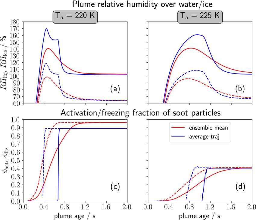
A. Bier et al.: Contrail formation trajectory studies                                                                        827

the Kelvin effect (Fig. B1a) and decreases with increasing κ       with Ṫ denoting the plume cooling rate. Using Eq. (4) we
due to the solution effect (Fig. B1b). The calculation of Sc is    obtain τfrz ' (a1 Ṫ )−1 .
described in Appendix B2.                                             The homogeneous freezing requirement will be fulfilled if
   The equilibrium saturation vapour pressures over the            the product of j = LWV · J and τfrz is unity. Using this re-
droplet (ice crystal) surface, used in Eqs. (2) and (7), are the   quirement, inserting the relations from above and rearranging
product of the saturation vapour pressure over a flat water        to T := Tfrz yields
(ice) surface and SK .                                                                "                          !    #
                                                                                   1       3 × 10⁻⁶ a1 Ṫ      3
                                                                   Tfrz (r, Ṫ ) =      ln                  · m s − a2 .      (6)
2.2.4    Condensational droplet growth                                             a1      4π (r 3 − rd 3 )
The droplet growth of activated soot particles is calcu-
lated according to Barrett and Clement (1988) and Kulmala             The homogeneous freezing temperature in contrails de-
(1993). In the steady state (small changes in the vapour flux)     clines with decreasing droplet radius and increasing cooling
and for spherical droplets, the single droplet mass growth         rate. As shown in Fig. 8 of Kärcher et al. (2015), Tfrz ranges
equation is given by                                               between around 230 and 232 K for typical droplet sizes (100–
                                                                   500 nm) at cruise altitude conditions.
dmw              4π r(ev − eK,w )
    =
 dt       Rv T             eK,w L2c −1
                 βm −1 +           β                               2.2.6    Depositional ice crystal growth
          Dv               Rv K̂T 2 t
                     ev − eK,w                                     The mass change of a single ice crystal (Mason, 1971) is
        = 4π r                       ,                      (2)
                 FM βm −1 + FH βt −1                               given by

where ev is the partial vapour pressure and eK,w equilibrium       dmi          4π CrDv βv−1 (ev − eK,i )
saturation vapour pressure over the droplet surface. Lc de-            =                                         ,            (7)
                                                                             Dv βv−1 Ld eK,i

                                                                    dt                          Ld
                                                                                                    − 1  + R   T
notes the specific latent heat for condensation/evaporation,                      −1 −1
                                                                              K̂βk βv T        Rv T          v
Dv the binary diffusion coefficient of air and water vapour,
K̂ the conductivity of air and Rv the specific gas constant        where C is the shape factor, r the equivalent volume radius
of vapour. The terms FM and FH represent the mass and              and Ld the specific latent heat for deposition/sublimation. In
heat diffusion term, with βm and βt denoting the transitional      our study, we set C to unity assuming spherical ice crystals as
correction factors calculated according to Fuchs and Sutugin       they are typically observed for young contrails (e.g. Schröder
(1971).                                                            et al., 2000). Since sedimentation is of low relevance during
                                                                   contrail formation, we neglect ventilation effects here. The
2.2.5    Homogeneous freezing                                      calculation of the transitional correction factors βv and βk is
                                                                   described in Appendix A.
We calculate the homogeneous freezing temperature (Tfrz ) of
a super-cooled droplet with radius r according to the method
of Kärcher et al. (2015). This method is suitable for a strong     2.3     Plume evolution and trajectory data
cooling situation typically occurring in a jet plume. We intro-
duce the nucleation rate as the number of droplets freezing        In this section, we first explain the plume evolution assum-
per unit time                                                      ing a mean state. Subsequently, we describe which kind of
                                                                   trajectory data we will use and how dilution, a measure for
j = J · LWV,                                                (3)    the air-to-fuel ratio and the volume of the plume, is derived
                                                                   from these data.
where J is the nucleation rate coefficient, and LWV =
4          3
3 π (r − rd ) is the liquid volume available for freezing. The     2.3.1    General plume dilution equations
temperature-dependent nucleation rate coefficient J is pa-
rameterized according to Riechers et al. (2013):                   The temporal evolution of the mass mixing ratio of a species
                                                                   χ(t) is given by (Kärcher, 1995; Kärcher, 1999)
J /(m−3 s−1 ) = 106 · exp(a1 T + a2 ),                      (4)
                                                                   χ̇(t) = −ωχ (χ(t) − χa ) + ξ (t),                          (8)
where a1 = 3.574 K−1 and a2 = 858.72 are empirical con-
stants. Assuming that the whole droplet freezes immediately
                                                                   where the first term describes the mixing of the hot exhaust
if ice nucleates within its volume, the pulse-like nature of j
                                                                   with ambient air, and the second term (ξ ) represents sink and
may be expressed by a characteristic freezing timescale
                                                                   source terms. The entrainment rate ωχ characterizes the dilu-
         ∂ ln j   ∂ ln J                                           tion, and χa is the ambient mass mixing ratio of the species.
 −1
τfrz =          '        Ṫ ,                               (5)    Applying the equation above to water vapour and setting up
           ∂t      ∂T

https://doi.org/10.5194/acp-22-823-2022                                                 Atmos. Chem. Phys., 22, 823–845, 2022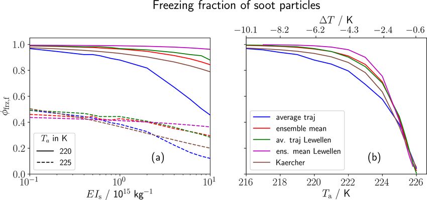
828 A. Bier et al.: Contrail formation trajectory studies
an analogous equation for the evolution of the plume temper- where ρ0 = Rpd Ta 0 is the air density, with pa denoting air pres-
ature (T ) yields sure, Rd the specific gas constant of dry air and mF the fuel
consumption (in kg m−1 ). The evolution of the plume area is
x˙v (t) = −ωv (xv (t) − xv,a ) + q̇PC (t), (9) given by
Ṫ (t) = −ωT (T (t) − Ta ) + ṪLH (t), (10)
ρ0 T (t)
A(t) = A0 · = A0 · . (16)
where Ta and xv,a are ambient temperature and vapour mass ρ(t)D(t) T0 D(t)
mixing ratio, respectively. The subscript LH relates to latent
heating, and PC stands for phase changes from water vapour In the numerical implementation, the ordinary differential
to liquid water or ice and vice versa. equations (ODE) like Eqs. (9) and (10) are discretized by
From the evolution of a passive tracer χp (t) (defined by a simple Euler forward scheme. Due to the linearity of the
Eq. 8 with ξ = 0), we can derive the entrainment rate ωp , ODEs, the implementation of an implicit Euler backward or a
second-order trapezoidal scheme is straight-forward, but we
χ˙p (t) find no improvement over the forward scheme. The source
ωp (t) = − , (11)
χp (t) − χp,a terms in the ODEs are provided by the LCM. In the LCM, the
computation involves summations over all SIPs with phase
and set ωv = ωp since water vapour is supposed to be diluted changes or water vapour uptake/release during the time step.
like a passive tracer. The entrainment rate characterizing the All model components (plume evolution ODE and LCM mi-
temperature change, ωT , differs from ωv by a factor called crophysics) use a time step of 0.001 s. This time step is suf-
the Lewis number, Le = ωv /ωT , which is the ratio of the ther- ficiently small to account for the fast diffusional growth at
mal and mass diffusivity. We set Le to 1, assuming that heat high plume supersaturations.
and mass diffusion proceed equally fast since turbulent ex-
change processes are dominating over molecular exchange
processes. Due to ωv = ωT , we skip the index from now on 2.3.2 Trajectory ensemble data
and simply use ω. The entrainment rate ω describes the in- Vancassel et al. (2014) used the LES solver FLUDILES to
stantaneous mixing strength. Integrating it over time, we ob- simulate the plume evolution in a 3D domain over 10 s start-
tain the plume dilution factor (Kärcher, 1995) ing behind the CFM56 engine nozzle of an A340-300 aircraft
t
Z
without treatment of the bypass. They sampled the plume
χp (t) − χp,a with 25 000 trajectories that were randomly positioned in-
D(t) = exp − ω(t 0 )dt 0 = , (12)
χp,0 − χp,a side the initial plume area A0 = π r0 2 with radius r0 = 0.5 m.
t0
We assume that all trajectories represent an equal share of the
where the subscript “0” refers to conditions at the engine exit plume, e.g. in terms of air mass and number of soot particles.
at time t0 := 0 s. For each trajectory, the temperature evolution T3D,k (t) has
At the engine exit, the emitted air is already a mixture of been tracked. We use these data to infer the dilution factor
ambient air and combustion products. The initial plume dilu- (or equivalently the entrainment rate) along each trajectory k
tion N̂0 can be derived from the temperature excess T0 − Ta : by assuming that temperature is a passive tracer:
Q(1 − η) T3D,k (t) − T3D,a
N̂0 = , (13) Dk (t) = . (17)
cp (T0 − Ta ) T3D,0 − T3D,a
where Q is the specific combustion heat, η the propulsion T3D,0 = 580 K and T3D,a = 220 K are the plume exit and
efficiency and cp = 1020 J(kg K)−1 an average heat capacity ambient temperature of the FLUDILES simulation. These
for dry air over a temperature range between around 200 and equations are only meaningful if T3D,k > T3D,a is fulfilled.
600 K (see derivation in Schumann, 1996). However, the LES temperature occasionally falls below T3D,a
The overall dilution N̂ generally increases with plume due to a pressure drop resulting from the interaction of the
age due to the continuous entrainment of ambient air and plume with the wake vortex. In the computation of ωk (t) or
is related to the dilution factor (this quantity decreases with Dk (t), we replace all values of T3D,k that are below T3D,a +
plume age) via with this lower limit. The threshold is chosen such that the
maximum dilution is still reasonable for a few seconds of
N̂(t) = N̂0 /D(t), (14) plume age (Dmin ≈ 2.5 × 10⁻³ ).
implying D0 = 1. In the FLUDILES simulation, the initial plume temper-
The initial plume area A0 results from mass conservation ature profile is based on the Crocco–Busemann relation
(Schumann et al., 1998): (White, 2005) and introduces a smooth radial transition be-
tween the plume and the environment. This ensures numeri-
N̂0 mF cal stability as gradients in prognostic variables that are too
A0 = , (15) strong are numerically intricate. This means that T3D,k (t0 )
ρ0
Atmos. Chem. Phys., 22, 823–845, 2022 https://doi.org/10.5194/acp-22-823-2022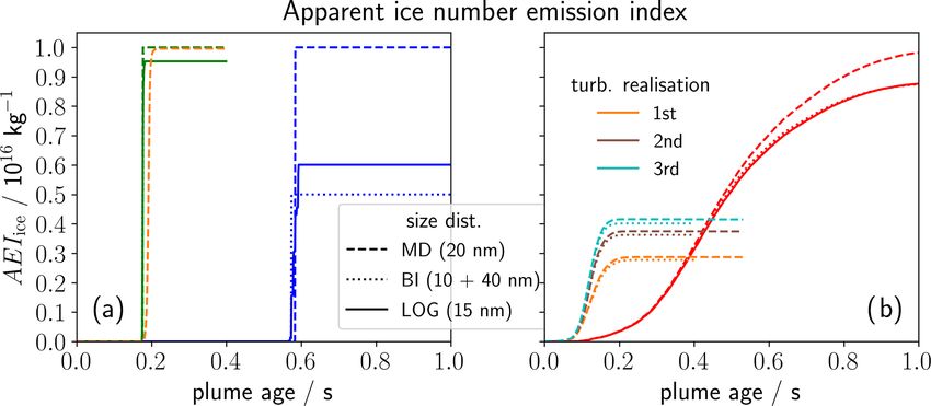
A. Bier et al.: Contrail formation trajectory studies                                                                                     829

Figure 1. Radial profiles of (a) temperature and (b–d) relative humidity over water RHliq in percent, (e) fraction of soot particles activating
into water droplets φact and (f) freezing to ice crystals φfrz . Whereas panels (a–c) show results from a simulation with switched-off contrail
microphysics, panels (d–f) show results from the baseline case with switched-on contrail microphysics. The contour plots in (b, d) show
RHliq over (r, t) space, where r is the absolute radial distance from the plume centre. The black line in (b) indicates the increasing plume
radius rp over time. All other panels show line plots at different plume ages (indicated by the legend), where the horizontal axis uses the
normalized radial distance r̃ = r/rp as coordinates.

only equals T3D,0 directly behind the nozzle exit centre and              tracer temperature”. Therefore, we underestimate dilution,
decreases down to around 400 K towards the plume edge (see                causing a later onset of contrail formation. This effect is par-
black line in Fig. 1a). These trajectories start with Dk,0 < 1            tially compensated for by the inhomogeneous initial temper-
and an accordingly higher initial dilution N̂k,0 . For simplic-           ature profile, implying that exhaust air parcels are already
ity, we mostly neglect this fact in the following description,            diluted near the plume edge.
but the initialization in this transition region is consistently             Basically, we only infer the dilution from the trajectory
treated in our model.                                                     data according to Eq. (17) and plug the corresponding en-
   The process of converting jet kinetic energy into thermal              trainment rate values into Eqs. (9) and (10) for each trajec-
energy is considered within the 3D simulations. This means                tory. For the radial plots presented later on, the coordinate
that the FLUDILES temperature is higher than a “passive

https://doi.org/10.5194/acp-22-823-2022                                                       Atmos. Chem. Phys., 22, 823–845, 2022
830                                                                         A. Bier et al.: Contrail formation trajectory studies

data of these trajectories are used, but the actual computa-      consumption, which is calculated by rearranging Eq. (15),
tions are independent of this type of information.                we obtain lower values than typical for this aircraft type
   Note that the ambient temperature Ta and plume temper-         since the initial plume radius given by FLUDILES is only
ature at engine exit T0 in Eqs. (9) and (10) are allowed to       0.5 m (Sect. 2.3.2). For given T0 , specific combustion heat
differ from T3D,a and T3D,0 used in Eq. (17). Similarly, the      and propulsion efficiency, we obtain N̂0 ≈ 75 according to
ambient and initial plume water vapour can be chosen inde-        Eq. (13). Note that the initial plume water vapour mixing ra-
pendently of the 3D data. In such a case, we basically only       tio is controlled by the water vapour emission index EIv :
use the information of the dilution and its variability.
   Moreover, a single mean state trajectory can be derived                       EIv         N̂0,k − 1
                                                                  xv,k (t0 ) =           +               xv,a ,                 (18)
from the trajectory ensemble. We determine the correspond-                       N̂0,k         N̂0,k
ing mean dilution DAT by averaging the preprocessed tem-
perature data over all 25 000 trajectories and plugging the       where the second term is the contribution of ambient humid-
average temperature evolution T 3D into Eq. (17).                 ity entering and exiting the engine. This term is less than 1 %
   There are other ways of computing the mean properties          of the total plume water vapour and, therefore, neglected in
of the trajectory ensemble. For instance, the mean temper-        our initialization.
ature can be a weighted average, where the cross-sections            Based on laboratory measurements, we prescribe log-
or masses of the trajectories are used as weights. The inter-     normally distributed soot particles with a geometric-mean
nal energy is conserved when a mass-conserving temperature        dry core radius (r d ) of 15 nm and geometric width of 1.6 (Ha-
average is used. The Supplement shows additional results for      gen et al., 1992; Petzold et al., 1999) and set the engine soot
a mass-conserving temperature average and contrasts them          number emission index (EIs ) to 1015 kg−1 as a typical value
with our default procedure.                                       for commercial aircraft (e.g. Schumann et al., 2002, 2013;
                                                                  Kleine et al., 2018). Furthermore, we assume the same hy-
                                                                  groscopicity parameter value (κs = 0.005) as in Kärcher et
2.4     Box model framework
                                                                  al. (2015).
We use the LCM box model, which is based on the 3D LCM               The overall number of emitted engine soot particles per
(introduced in Sect. 2.1) and has been extended for the con-      flight distance is given by
trail formation microphysics. Similarly to Paoli et al. (2008),
we either perform a single box model run with an aver-            Ns,tot = EIs · mF .                                           (19)
age dilution (labelled “average traj”) or an ensemble of box
model runs for the trajectory dilution data (labelled “ensem-
                                                                     Table 2 summarizes the parameter variations (PVs) that
ble mean”). The simulated time tsim is 2 s. In the following,
                                                                  investigate the sensitivity of contrail formation to soot prop-
we describe the initial conditions (Sect. 2.4.1) and introduce
                                                                  erties (PV1–PV4) and ambient conditions (PV5/PV6). In
important diagnostics, including explanations about the av-
                                                                  the first two PVs, we either vary EIs or r d . Flight mea-
eraging procedure for ensemble mean runs (Sect. 2.4.2).
                                                                  surements have shown that a 50 : 50 mixing of conventional
                                                                  kerosene with a biofuel causes a decrease in EIs by around
2.4.1    Initial conditions                                       50 % (Moore et al., 2017). Moreover, they find a decrease
                                                                  of the average soot particle size. This is because the switch
Table 1 summarizes initial conditions of our baseline sce-
                                                                  to alternative fuels leads to a reduced number of primary
nario, which are described in the following. The plume exit
                                                                  soot spherules. The subsequent coagulation between those
temperature (near the plume centre) is set to 580 K. We
                                                                  spherules decreases, and the final soot aggregates are smaller
prescribe an ambient temperature of either 220 K (baseline
                                                                  on average. Therefore, in PV3, we vary both EIs and r d and
case) or 225 K (near-threshold case). The baseline SA thresh-
                                                                  combine a 50 % reduction in EIs with a reduction in r d to
old temperature (2G ) is 226.2 K for the given atmospheric
                                                                  12.5 nm. In PV4, we change the hygroscopicity parameter
conditions and engine/fuel properties. The prescribed ambi-
                                                                  of soot particles in a reasonable range between 0.001 and
ent relative humidity over ice, RHice,a , determines the am-
                                                                  0.01 (Markus Petters, personal communication, 2019). Fi-
bient water vapour mixing ratio xv,a being proportional to
                                                                  nally, we study the variation of contrail properties with am-
RHice,a · es,ice (Ta ). We use RHice,a = 120 % for the baseline
                                                                  bient temperature Ta (PV5) and relative humidity over ice
case.
                                                                  RHice,a (PV6).
   Engine and fuel parameters such as specific combustion
heat, propulsion efficiency and water vapour mass emis-
sion index are prescribed consistently with the trajectory        2.4.2    Diagnostics
data set-up and have values according to an A340-300 air-         Here, we introduce diagnostics that are used to evaluate the
craft at cruise speed (Table 1). These parameters are kept        simulations.
constant for all sensitivity studies, even though they can
slightly change with varying ambient conditions. For the fuel

Atmos. Chem. Phys., 22, 823–845, 2022                                                        https://doi.org/10.5194/acp-22-823-2022
A. Bier et al.: Contrail formation trajectory studies 831
Table 1. Baseline parameters of all regular LCM simulations (first three rows) and those corresponding to the box model set-up of Lewellen
(2020) (last three rows). Hereby, Mono20 stands for a monodisperse distribution with rd = 20 nm and Bi10/40 for a bidisperse distribution
with a 50/50 mixture of 10 and 40 nm particles.
Ambient conditions Fuel/engine properties Engine exit conditions Soot particle properties Numerical parameters
Ta = 220 K EIv = 1.26 kg kg−1 T0 = 580 K EIs = 1015 kg−1 tsim = 2 s
pa = 240 hPa Q = 4.3 × 10⁷ J kg−1 N̂0 ≈ 75 r d = 15 nm dt = 0.001 s
RHice,a = 120 % η = 0.36 A0 = 0.25π m2 κs = 0.005 NSIP = 130
Ta = 218.8 K EIv = 1.25 kg kg−1 T0 ≈ 480 K EIs = 1016 kg−1 tsim = 1 s
pa = 238.4 hPa Q = 4.29 × 10⁷ J kg−1 N̂0 ≈ 92 Mono20 or Bi10/40 dt = 0.001 s
RHice,a = 110 % η = 0.325 A0 = 0.31 m2 κs = 0.005 NSIP = 130
Table 2. Parameter variations (PVs) of various soot properties and ambient conditions. The values in bold depict the default baseline
parameter, and EIs,ref is the baseline soot number emission index.
PV1: EIs /EIs,ref PV2: r d /nm PV3: EIs /EIs,ref and r d PV4: κs PV5: Ta /K PV6: RHice,a /%
0.5 12.5 0.5 and 12.5 0.001 215 100
1.0 15.0 1.0 and 15.0 0.005 220 120
2.0 20.0 2.0 and 20.0 0.01 225 140
The fraction of soot particles activated into water droplets 3 Results
(φact ) or frozen to ice crystals (φfrz ) is given by
PNSIP In this section, we first describe the spatio-temporal evolution
ζi,act/frz Ns,i of thermodynamic and contrail properties during the forma-
φact/frz = i=1 , (20)
Ns,tot tion stage (Sect. 3.1). We then analyse the temporal evolution
where ζi characterizes whether soot particles (ζi,act = ζi,frz = of contrail properties depending on different soot properties
0) represented by a SIP i have turned into water droplets and atmospheric parameters in Sect. 3.2. Finally, we summa-
(ζi,act = 1 and ζi,frz = 0) or ice crystals (ζi,act = ζi,frz = 1). rize our results by studying the sensitivity of final contrail
Note that we classify ice crystals as activated; hence we get ice crystal numbers to ambient temperature and relevant soot
0 ≤ φfrz ≤ φact ≤ 1. properties. Our simulations are based on the FLUDILES di-
We introduce the apparent ice number emission index, lution data, and we particularly compare simulations using
AEIice , as a measure of the number of formed ice crystals the full trajectory ensemble and a single average trajectory.
per fuel mass burnt. Since we consider only soot as exhaust
particles in our study, AEIice is simply given by the product 3.1 Spatial variation of contrail properties
of φfrz and EIs .
The first two rows of Fig. 1 depict the spatio-temporal evolu-
Furthermore, we define the effective radius of the soot–
tion of temperature and relative humidity. The plume radius
droplet–ice number distribution as
(black line in Fig. 1b) is evaluated as the distance of the most
PNSIP 3
ri · Ns,i remote trajectory from the plume centre at given plume age t.
reff = Pi=1NSIP 2
. (21) The jet plume expands from an initial radius of 0.5 m towards
i=1 ri · Ns,i around 7.5 m after t = 1 s. Figure 1a shows the radial profiles
Typically, reff is a quantity that is relevant in radiation of temperature for different plume ages. In the very begin-
problems. Here, we prefer reff over the ordinary mean radius ning (black), the plume centre is not affected by entrainment,
since the time evolution is smoother, and there is no need to and the core temperature remains at its initial value. In the
specify the total particle number. outer areas, the temperature profile is smoothed according to
For ensemble mean values, intensive and extensive phys- the Crocco–Busemann profile. The radial temperature gradi-
ical quantities are mass-weighted averages and sums of tra- ent is initially large (nearly a temperature decrease of 300 K
jectory ensemble values, respectively. For quantities that are at t = 0.05 s) and decreases with increasing plume age as the
defined as ratios like the effective radius or relative humidity, plume centre cools. Later on, the absolute changes in tem-
first the averages of the quantities that appear in the denom- perature, spatially and temporally, decrease continuously.
inator and nominator are computed, and then the ratio over Figure 1b shows the radial–temporal RHliq distribution of
those averaged quantities is taken. Note that the mass weights a simulation with switched-off contrail microphysics, where
cancel out in the definitions of φact/frz and reff . water vapour behaves like a passive tracer. We call the dis-
https://doi.org/10.5194/acp-22-823-2022 Atmos. Chem. Phys., 22, 823–845, 2022832 A. Bier et al.: Contrail formation trajectory studies
played quantity the hypothetical RHliq ; it increases with in- rapid droplet formation on soot particles. Thereby, φact in-
creasing plume age (at least for t ≤ 0.5 s) and decreasing creases quasi pulse-like from zero to its final value. Subse-
plume temperature due to the non-linearity of the satura- quently, RHliq decreases and approaches 100 %. After 0.7 s
tion vapour pressure. Since plume cooling starts earlier and the droplets freeze rapidly into ice crystals, and the deposi-
proceeds faster near the plume edge, water saturation is sur- tional ice crystal growth causes a steeper decrease in RHliq
passed earlier in this region (after 0.25 s) than in the plume until ice saturation is reached (see blue line in Fig. 2a). Re-
centre (after 0.5 s). For a fixed plume age up to t = 0.5 s, garding the ensemble mean evolution, the fraction of soot
the hypothetical RHliq increases with increasing radial dis- particles forming droplets/ice crystals increases smoothly
tance for r̃ ≤ 0.6 as is apparent from Fig. 1c. At higher plume over a certain time window. This is explained as follows: the
ages and radial distances, the dependency of the hypothetical spatial variability in RHliq is quite large (Fig. 1d) due to a sys-
RHliq on r, t reverses. tematic radial gradient and superposed turbulent deviations.
Figure 1d–f show results of a simulation with switched-on Therefore, droplet and ice crystal formation occurs for dif-
contrail microphysics. As soon as droplet formation on soot ferent trajectories at a different plume age, mostly depending
particles is initiated (i.e. after plume relative humidity ex- on the radial distance to the plume centre (Fig. 1e and f). Al-
ceeds at least water saturation), the further increase in RHliq though the ensemble mean features a smaller RH peak value
is inhibited due to condensational loss of water vapour. The than the average traj evolution, a larger fraction of soot par-
subsequent rapid decrease in RHliq (first at the plume edge ticles forms ice crystals (96 % vs. 88 %).
and later on in the plume centre) is due to ice crystal forma- In the near-threshold case (right column), Tsat ≈ 236 K is
tion and subsequent depositional growth. After around 1 s, lower and closer to Ta . Hence, water saturation is reached
the relative humidity with respect to ice reaches values of at a higher plume age when the cooling rates are already
100 %, which translates into water-subsaturated plume con- lower. Additionally, the peak RH values are clearly reduced.
ditions. Figure 1e shows the fraction of activated soot parti- According to the evolution of the plume relative humidity,
cles (φact ). According to the evolution in plume relative hu- droplet and ice crystal formation on soot particles is initi-
midity, soot particles activate into water droplets first near ated a few tenths of a second later compared to Ta = 220 K
the plume edge and afterwards in the plume centre. Water ((Fig. 1d). The time between the activation of the first
saturation in the plume is first reached for Tsat ≈ 240 K so droplets and the freezing of the last droplets is also longer
that below those temperatures soot particles may form wa- (1.6 versus 1.2 s). The final φact and φfrz values are clearly
ter droplets and grow further by condensation. The homoge- reduced relative to the baseline case since only the larger
neous freezing of the super-cooled water droplets typically soot particles can activate into water droplets due to the de-
occurs at Tfrz ≈ 230–232 K depending on the droplet size and creased peak RHliq . Again, the ensemble mean evolution dis-
the cooling rate. Figure 1f shows the fraction of soot par- plays slightly higher final φfrz values than the average traj.
ticles that turned into ice crystals (φfrz ). The radial profiles A closer look at the average traj evolution of the near-
of φfrz behave similarly to the corresponding profiles of φact threshold case reveals that φact is not a monotonically in-
but with a time lag of around 0.2 s. In the outer part with creasing function and that the final φfrz value is lower than
r̃ > 0.5, basically all soot particles have become ice crystals the φact value at some intermediate time (in this example at
after around 0.6 s. At t = 0.6–0.8 s, the profiles exhibit local t = 0.9 s). This is explained as follows: the largest soot par-
minima at r̃ ≈ 0.2, which results from the minimum in RHliq ticles are activated first, and over time smaller soot particles
after around 0.7 s (Fig. 1b). grow large enough to be considered activated as well. How-
ever soon after, RHliq drops below SK (for the smaller soot
particles) as condensational growth removes water vapour.
3.2 Temporal evolution of contrail properties Those particles shrink, such that their radius drops below the
3.2.1 Mean state trajectory versus trajectory ensemble activation radius. Once the largest water droplets freeze, de-
positional growth leads to a fast depletion of water vapour.
We employ the box model in two different frameworks as Again, the smallest of the currently activated droplets face
outlined in Sect. 2.4. In the average traj framework, a single water-subsaturated conditions and also become deactivated
box model run with an average dilution is performed. In the (at around t = 1.25 s). We will encounter this “deactivation
ensemble mean framework, box model runs are carried out phenomenon” later again. Even though it is not visible in the
for the complete set of 25 000 trajectories. ensemble mean evolution, this deactivation phenomenon also
Figure 2 compares the plume relative humidity (top row) occurs for most trajectories of the ensemble runs.
and the activation–freezing fraction between both frame-
works. This is done for baseline conditions (Fig. 2a and c, 3.2.2 Variation with soot properties
Ta = 220 K) and a near-threshold case (Fig. 2b and d,
Ta = 225 K with |Ta − 2G | ≈ 1.5 K). First, we analyse the In this section, we investigate the sensitivity of contrail for-
baseline case. For the average traj, RHliq surpasses water mation to various soot properties. Figure 3 presents results
saturation after around 0.4 s and leads immediately to a of the sensitivity studies PV1 to PV4. As in the previous sec-
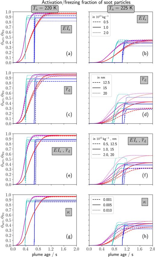
Atmos. Chem. Phys., 22, 823–845, 2022 https://doi.org/10.5194/acp-22-823-2022A. Bier et al.: Contrail formation trajectory studies 833 Figure 2. Temporal evolution of (a, b) plume relative humidity over water (dashed) and ice (solid) and of (c, d) the fraction of soot particles activating into water droplets (dashed) and forming ice crystals (solid). The left column (a, c) shows the baseline case with ambient temperature Ta = 220 K and the right column (b, d) the near-threshold case with Ta = 225 K. Results are shown for the ensemble mean (red) and the average traj (blue) evolution. tion, the baseline and near-threshold temperature cases are lution are more sensitive to the variation of r d and κ than considered. We first analyse the baseline temperature case for Ta = 220 K. This is because of two basic reasons: first, (Ta = 220 K; Fig. 3a, c, e and g). The ensemble mean results the critical saturation ratio for the activation of soot particles reveal that the temporal evolution of the activation fraction varies non-linearly with the soot core size (due to the non- φact and freezing fraction φfrz hardly changes with any varia- linear Kelvin term), displaying a strong change for rd < 10 m tion of the soot properties. In the average traj framework, the (Fig. B1a). This means that far away from the formation sensitivity to soot properties is slightly higher. There, the ac- threshold, larger changes of r d and κ are necessary to af- tivation and freezing fraction moderately increases with de- fect the activation of the several nanometre-sized soot parti- creasing EIs (Fig. 3a) and increasing r d (Fig. 3b). A higher cles. Second, these small soot particles are at the tail of the number of soot particles leads to a faster depletion of plume size-distribution, and, therefore, their activation only makes relative humidity, prohibiting the activation of smaller parti- a low contribution to the overall φact . In the near-threshold cles. Likewise, a decrease of r d reduces the number of soot case, only the larger soot particles (rd &20 nm) can form wa- particles that manage to be activated. Changing the two pa- ter droplets. This activation threshold is close to r d , which rameters, EIs and r d , simultaneously (Fig. 3c), the effects on simultaneously defines the maximum of the log-normal size φact and φfrz more or less cancel out, resulting in an almost distribution. Hence, changing r d or κ has a significantly negligible effect. The variation of φfrz with the hygroscop- higher impact on φact for Ta = 225 K than for lower ambi- icity of soot particles (Fig. 3d) displays the lowest impact ent temperature. within the considered parameter range. Note that the aver- Again, we find a stronger sensitivity to rd (Fig. 3d) than age traj simulations with higher prescribed EIs (dotted cyan for κ (Fig. 3h) Interestingly, the ensemble mean simulations lines) exhibit the aforementioned deactivation phenomenon. show larger rd - and κ-induced variations in φfrz in the end In the near-threshold scenario, the φact and φfrz values than the average traj simulations, which is opposite to what are clearly lower due to decreased plume water supersatu- we saw in Fig. 3c and g. This is mainly due to the deacti- ration (Sect. 3.2.1). While the variation with EIs (Fig. 3b) vation phenomenon. In the combined variation of EIs and r d is still low, both average traj and the ensemble mean evo- (Fig. 3f), the impact of r d on φact and φfrz dominates over that https://doi.org/10.5194/acp-22-823-2022 Atmos. Chem. Phys., 22, 823–845, 2022
834                                                                                  A. Bier et al.: Contrail formation trajectory studies

Figure 3. Temporal evolution of the fraction of soot particles activating into water droplets φact (cyan and magenta) and forming ice crystals
φfrz (blue and red) for a variation of the soot number emission index EIs (a, b), geometric-mean dry core radius r d (c, d), a combined variation
of EIs and r d (e, f) and a variation of the hygroscopicity parameter κ (g, h). The left column (a, c, e, g) shows the baseline (Ta = 220 K) and
the right column (b, d, f, h) a near-threshold case (Ta = 225 K). The magenta and red lines show the ensemble mean and the cyan and blue
lines the average traj results. The different line types (see legends on the right column) represent the according soot parameter variations
(PV1–PV4).

Atmos. Chem. Phys., 22, 823–845, 2022                                                           https://doi.org/10.5194/acp-22-823-2022
A. Bier et al.: Contrail formation trajectory studies                                                                           835

of EIs . Halving the EIs value and decreasing r d to 12.5 nm        2G from 226.2 to 225.5 K so that those contrails form only
leads to a decrease in φfrz from 0.41 to 0.31 and translates        0.5 K below the SA threshold temperature, and maximum
into a decrease of AEIice even by 62 % (instead of around           plume water supersaturation is only a few percent. Analo-
50 % if only the EIs value is halved).                              gously, more ice crystals form for RHice,a = 140 % as 2G ,
   Furthermore, we have investigated the sensitivity of con-        and hence |Ta − 2G | ≈ 3 K is higher.
trail formation to the geometric width of the soot particle size       Our results highlight that the sensitivity of contrail ice nu-
distribution σ (not shown): in contrast to the variation with r d   cleation to atmospheric parameters is large near the contrail
and κ, there is a negligible impact near the contrail formation     formation threshold, which is consistent with previous stud-
threshold (Ta = 225 K). This is because the activation of soot      ies (e.g. Kärcher and Yu, 2009; Kärcher et al., 2015; Bier and
particles with dry core radii below r d is already inhibited due    Burkhardt, 2019). Therefore, it is meaningful to display the
to the Kelvin effect. For our baseline case, a higher fraction      variation of the nucleated contrail ice crystal number with
of soot particles forms ice crystals if the geometric width is      1T := Ta − 2G as well (see next section).
reduced. This is due to the fact that the smallest soot parti-
cles within the size distribution become larger and hence can       3.3   Final ice crystal number
be activated more easily. Decreasing (increasing) geometric
width from 1.6 to 0.8 (2.4) causes a decrease (increase) in         In the following, we aim at summarizing the results from the
φfrz from 0.88 to 0.83 (0.98) for the average traj and from         previous sensitivity studies. We analyse the sensitivity of fi-
0.96 to 0.93 (0.99) for the ensemble mean.                          nal contrail ice crystal numbers to ambient temperature and
                                                                    relevant soot properties. Thereby, we display both the freez-
3.2.3   Sensitivity to ambient conditions
                                                                    ing fraction (Fig. 5a, c and e) and the absolute ice crystal
                                                                    number in terms of AEIi,f (Fig. 5b, d and f). The latter is
In this subsection, we study the dependence of contrail for-        shown only for sensitivities with varying EIs since otherwise
mation on ambient conditions. We vary the ambient temper-           there is simply a linear relationship between φfrz,f and AEIi,f .
ature Ta and background relative humidity over ice RHice,a             The freezing fraction in general decreases with increas-
(see PV5 and PV6 in Table 2).                                       ing EIs (Fig. 5a) because the plume humidity is depleted
   Figure 4a and b display the variation of ambient temper-         faster at higher exhaust particle number concentrations and
ature Ta at default RHice,a = 120 %. As already explained           also distributed among more ice crystals. Hence, the smaller
above, a change of Ta affects the contrail formation time and       soot particles do not manage to form contrail ice crystals.
the number of soot particles turning into ice crystals. The         In our model set-up, the ensemble mean φfrz,f only slightly
lower the Ta , the earlier that water saturation is first reached   changes with EIs , confirming the low sensitivity pointed out
in the plume and the higher the attained peak water supersat-       in Sect. 3.2.2. Accordingly, the ensemble mean AEIi,f in-
uration is. Hence, reducing Ta to 215 K, droplet and ice crys-      creases nearly linearly with increasing EIs . The average traj
tal formation is initiated earlier, and more ice crystals form      φfrz,f evolution (blue curve) features a stronger decrease than
(Fig. 4a). The results for Ta = 220 and 225 K have already          the ensemble mean, in particular for the higher soot number
been described in Sect. 3.2.2. Thereby, the difference in φfrz      emissions (EIs > 1015 kg−1 ). This is due to the deactivation
is significantly larger between 225 (dotted) and 220 K (solid)      phenomenon explained in Sect. 3.2.2. Therefore, the increase
than that between 220 and 215 K (dashed).                           in AEIi,f with rising EIs flattens in the average traj case.
   The evolution of the effective radius reff in Fig. 4b shows         Figure 5c displays the variation of φfrz,f with ambient tem-
a steep increase from the moment when the first droplets are        perature Ta (lower label) and the difference between Ta and
activated. The increase slows down in most cases and is ac-         2G (1T , upper label). Note that the relation between Ta and
celerated again once the droplets freeze. The curves level off      1T is not purely linear since the ambient relative humid-
as soon as ice saturation is reached in the plume. This hap-        ity over water varies with Ta at fixed RHice,a , and, hence,
pens after around 1 s for the lower Ta and after around 2 s         2G slightly changes as well. Near the contrail formation
for Ta = 225 K. The final reff values hardly change between         threshold (i.e. |1T |. 3–4 K), φfrz,f strongly increases with
Ta = 215 and 220 K and between the average traj and the             rising |1T |. This is because the maximum plume water su-
ensemble mean. Only for Ta = 225 K are higher values at-            persaturation increases, and more and more soot particles
tained. This is because the absolute amount of ambient water        manage to activate into water droplets. Below Ta = 220 K
vapour is higher for higher Ta and gets distributed among           (|1T | > 6 K), more than 90 % of the soot particles turn
fewer ice crystals.                                                 into ice crystals for our parameter setting so that AEIi,f ap-
   Figure 4c and d show the variation of RHice,a . For Ta =         proaches EIs . The average traj simulation produces some-
220 K (Fig. 4c), contrail ice nucleation is not at all affected     what lower φfrz,f values than the ensemble mean simulation.
by the variation of RHice,a . In contrast, the sensitivity of       Furthermore, low soot simulations (with EIs reduced by 80 %
φfrz to RHice,a is very high for Ta = 225 K. At ice satura-         relative to the baseline case) feature a similar evolution in
tion (dotted line), only few ice crystals form (φfrz < 10 %).       φfrz,f and a smaller difference between the average traj and
This is because a decrease in RHice,a causes a decrease in          the ensemble mean (not shown).

https://doi.org/10.5194/acp-22-823-2022                                                Atmos. Chem. Phys., 22, 823–845, 2022
You can also read