Implementing the Water, HEat and Transport model in GEOframe (WHETGEO-1D v.1.0): algorithms, informatics, design patterns, open science features ...
←
→
Page content transcription
If your browser does not render page correctly, please read the page content below
Geosci. Model Dev., 15, 75–104, 2022
https://doi.org/10.5194/gmd-15-75-2022
© Author(s) 2022. This work is distributed under
the Creative Commons Attribution 4.0 License.

Implementing the Water, HEat and Transport model in GEOframe
(WHETGEO-1D v.1.0): algorithms, informatics, design patterns,
open science features, and 1D deployment
Niccolò Tubini1 and Riccardo Rigon2
1 Department    of Civil, Environmental and Mechanical Engineering, University of Trento, Via Mesiano 77, 38123 Trento, Italy
2 Center   Agriculture Food Environment, University of Trento, Via Mesiano 77, 38123 Trento, Italy

Correspondence: Niccolò Tubini (niccolo.tubini@unitn.it)

Received: 19 May 2021 – Discussion started: 21 July 2021
Revised: 25 October 2021 – Accepted: 22 November 2021 – Published: 7 January 2022

Abstract. This paper presents WHETGEO and its 1D de-              regulate the natural habitat and determine the availability of
ployment: a new physically based model simulating the wa-         life-sustaining resources (National Research Council, 2001).
ter and energy budgets in a soil column. The purpose of this      Clear interest in studying the CZ is spurred on by ever-
contribution is twofold. First, we discuss the mathematical       increasing pressure due to growth in the human population
and numerical issues involved in solving the Richardson–          and climatic changes. Central to simulating the processes in
Richards equation, conventionally known as the Richards           the CZ is the study of soil moisture dynamics (Clark et al.,
equation, and the heat equation in heterogeneous soils. In        2015a; Tubini et al., 2021b). In the following we suggest that
particular, for the Richardson–Richards equation (R 2 ) we        studying the CZ requires tools that are not yet readily avail-
take advantage of the nested Newton–Casulli–Zanolli (NCZ)         able to researchers; then we propose one of our own. These
algorithm that ensures the convergence of the numerical so-       tools should be flexible enough to allow the quick embedding
lution in any condition. Second, starting from numerical and      of advancements in science.
modelling needs, we present the design of software that is
intended to be the first building block of a new customizable     1.1   Setting up the water budget
land-surface model that is integrated with process-based hy-
drology. WHETGEO is developed as an open-source code,             It is generally accepted in the field that the motion of wa-
adopting the object-oriented paradigm and a generic pro-          ter in soil is regulated by a Darcian–Stokesian flow, mean-
gramming approach in order to improve its usability and           ing that any force is immediately dissipated and water un-
expandability. WHETGEO is fully integrated into the GE-           der a gradient of generalized forces acquires a velocity (the
Oframe/OMS3 system, allowing the use of the many ancil-           Darcy velocity) which is linearly proportional to the gradient
lary tools it provides. Finally, the paper presents the 1D de-    of the generalized force. This law is known as the Darcy–
ployment of WHETGEO, WHETGEO-1D, which has been                   Buckingham law and reads
tested against the available analytical solutions presented in    J = K(θ )∇ (ψ + z) ,                                       (1)
the Appendix.
                                                                  where the forces acting are gravity (z; L) and the matric po-
                                                                  tential ψ [L] and where J [L T−1 ] is the Darcian flux, K
                                                                  [L T−1 ] is the hydraulic conductivity, θ [L3 L−3 ] is the di-
1   Introduction                                                  mensionless volumetric water content, ∇ [L−1 ] is the gra-
                                                                  dient operator, and z [L] is the vertical coordinate positive-
The Earth’s critical zone (CZ) is defined as the heteroge-        upward. The assumptions under which such a law is derived
neous near-surface environment in which complex interac-          from Newton’s law are presented in Whitaker (1986) and
tions involving rock, soil, water, air, and living organisms      Di Nucci (2014). The hydraulic conductivity depends on soil

Published by Copernicus Publications on behalf of the European Geosciences Union.
76                                                                                    N. Tubini and R. Rigon: WHETGEO-1D

type (texture and structure) and water content, while the ther-       5. Capillary forces are not the only ones acting at the mi-
modynamic forces must be understood as gradients of the                  croscale (Lu, 2016). In fact, measured suction values are
chemical potential of water, which, in turn, can be split in             far below pressures that can be sustained by capillarity
matric potential, osmotic potential, and other potentials (No-           alone.
bel, 1999, chap. 2). However, in Eq. (1) we consider only
the action of the matric potential. On the basis of the law of        6. Temperature affects water viscosity; infiltration is faster
motion in Eq. (1), the mass conservation reads                           at warm temperatures and slower at cold ones (Con-
                                                                         stantz and Murphy, 1991).
∂θ
   = ∇ · (K(θ )∇ (ψ + z)) ,                                   (2)     7. In high-latitude and high-elevation environments, soils
∂t
                                                                         may be subject to freezing and thawing processes which
where ∇· [L−1 ] is the divergence operator. Equation (2) is              affect pore volume and water dynamics (Dall’Amico
usually known as the Richards equation (Richards, 1931)                  et al., 2011).
but was previously formulated by Richardson (1922). There-
fore, in the following we call it the R 2 equation to remind         These facts certainly do not threaten the nature of mass
the reader of this double origin. There are very informative         conservation in Eq. (2). However, they can certainly alter
reviews that cover its general, historical, and numerical as-        the statistics which generate the closure equations, i.e. the
pects, such as Paniconi and Putti (2015), Farthing and Ogden         SWRCs we currently use.
(2017), and Zha et al. (2019). Therefore, it is not deemed nec-
essary to further summarize the matter here. The R 2 equation          – Requirement I – without entering into further details,
is a function of two variables, θ and ψ, and its resolution re-          we can observe that the aforementioned issues have
quires another relation between these two quantities. This re-           consequences that would require new software to in-
lation is known as soil water retention curves (SWRCs), writ-            clude the possibility of adopting new parameterizations
ten in the plural because we have many SWRCs depending                   of SWRCs and hydraulic conductivity quickly, easily,
on soil characteristics. The reader may be aware that the R 2            and neatly.
is an exact description of unsaturated flow only if we assume
that soil is a bundle of capillaries and that the largest capil-     1.2   The three or four worlds
laries drain first and are filled last (Mualem, 1976). In fact, in
                                                                     The flow of water obeys the general laws of physics for con-
this case a relation can be obtained between the radius of the
                                                                     servation of mass and momentum, but, since the seminal
capillaries and the suction, which was fully derived (Kosugi,
                                                                     works of Freeze and Harlan (1969), the scientific commu-
1999). However, there are various reasons to take the capil-
                                                                     nity has split up (Furman, 2008) into three groups: ground-
lary bundle concept as a rough approximation of natural soil.
                                                                     water people, vadose zone scientists, and surface water hy-
Some of the issues are enumerated below.
                                                                     drologists. This compartmentalization of the scientific com-
  1. Firstly, pores in soils are not bundles of well-defined         munity was fostered to deepen the knowledge within single
     capillaries of a single diameter; in fact, they can have        branches, with the interactions between the different parts
     quite random structures, as revealed, for instance, by to-      having been governed in models by assigning boundary con-
     mography (Yang et al., 2018).                                   ditions (Furman, 2008). However, these boundary conditions
                                                                     are intrinsically inadequate and inappropriate in representing
  2. Secondly, logic and pore scale simulations, as in Tomin         the physics of interactions between different domains whose
     and Lunati (2016), for example, indicate that fluids fill       interactions depend strictly on the state of the system. When
     the cavities where they fall, and only eventually are they      these conditions are prescribed a priori (Furman, 2008), the
     redistributed according to the microstructure of the soil;      proper dynamics of the CZ fluxes cannot be obtained. There
     that is to say that fluids do not move instantaneously          is a need to overcome this situation.
     from the largest pores to the smallest ones.
                                                                       – Requirement II – the boundary conditions hard-wired
  3. A set of relatively large pores can, in certain conditions,
                                                                         into algorithm implementation should be removed in
     preferentially drive the flow of water in a short timescale
                                                                         favour of a simultaneous treatment of the three compart-
     according to laminar viscous flow driven by gravity be-
                                                                         ments (surface waters, vadose zone, and groundwater).
     fore any redistribution happens (Germann and Beven,
     1981).                                                             Fortunately, Šimůnek et al. (2012) found the way to
                                                                     smoothly extend the Richards equation into the groundwa-
  4. The role of living matter, such as bacteria, animals,
                                                                     ter equation. This and other similar approaches are now used
     fungi, vegetation, and roots, is usually eliminated from
                                                                     in various codes, such as Hydrus, ParFlow (Ashby and Fal-
     the hydrological picture, but it should have a relevant
                                                                     gout, 1996; Jones and Woodward, 2001; Kollet and Maxwell,
     place (Benard et al., 2019).
                                                                     2006), CATHY (Paniconi and Wood, 1993; Paniconi and
In addition are the following points.                                Putti, 1994), and GEOtop 2.0 (Rigon et al., 2006a; Endrizzi

Geosci. Model Dev., 15, 75–104, 2022                                                    https://doi.org/10.5194/gmd-15-75-2022
N. Tubini and R. Rigon: WHETGEO-1D                                                                                                77

et al., 2014). To extend the R 2 equation into the saturated         acceleration of gravity, and ν [L2 T−1 ] is the kinematic vis-
domain it is necessary to include the contribution of ground-        cosity of the liquid. Thus, for constant θ , variations in K(θ )
water storativity due to matrix and fluid compressibility. The       due to temperature can be accounted for as (Constantz and
common approach is to write the R 2 equation as                      Murphy, 1991)
∂θ      θ ∂θ                                                                                 ν(T1 )
   + Ss       = ∇ · (K(ψ)∇(ψ + z)) ,                          (3)    K(θ, T2 ) = K(θ, T1 )          ,                            (8)
∂t      θs ∂t                                                                                ν(T2 )
where Ss [L−1 ] is the specific storage coefficient, defined as      In Eq. (8), T1 is a reference temperature, while T2 is the soil
Ss = ρg(nβ + α),                                              (4)    water temperature. Temperature is also responsible for the
                                                                     phase change of water (point 7), and because of pore ice, as
with ρ [M L−3 ] being the water density, g [L T−2 ] gravita-         well as excess ice, infiltration rates and subsurface flows are
tional acceleration, n [L3 L−3 ] the soil porosity, β [L T2 M−1 ]    significantly modified (Walvoord et al., 2012).
the liquid compressibility, and α [L T2 M−1 ] the matrix com-
pressibility. On the left-hand side of Eq. (3), the first term         – Requirement III – to account for thermodynamic ef-
accounts for changes in liquid saturation, while the second              fects, temperature should at least be present in the R 2
term accounts for the compression or expansion of the porous             equation as a parameter, as in Eq. (8). However, for a
medium and the water. The left-hand-side term in Eq. (3) can             more accurate approximation of the water dynamics, the
be rewritten as                                                          option to solve the water and energy budgets simultane-
                                                                       ously must be present.
         θ ∂ψ
  c + Ss         ,                                           (5)
         θs ∂t                                                       Soil thermal properties are important physical parameters in
                                                                     modelling land-surface processes (Dai et al., 2019) since they
where c [L−1 ] is the water retention capacity. Comparing            control the partitioning of energy at the soil surface and its
the two terms in brackets, we can see that for ψ < 0, then           redistribution within the soil (Ochsner et al., 2001). For a
c  Ss θθs ; this means that under unsaturated conditions, the       multi-phase material like soil, their definition is always prob-
contribution of the specific storage is negligible. Whereas          lematic since they depend on the physical properties of each
when the soil is saturated and ψ > 0, then c = 0 and there-          phase and their variations (Dong et al., 2015; Dai et al., 2019;
fore what counts is the specific storage. Because of this, it is     Nicolsky and Romanovsky, 2018). In the literature different
possible to account for groundwater specific storage simply          models have been proposed with such a scope, and further
by modifying the SWRC as                                             studies on it are recommended (Dai et al., 2019): nonethe-
         (                                                           less, when considering the phase change of water, the es-
            θ (ψ)      if ψ < 0
θ(ψ) =                                                      (6)      timation of the unfrozen and frozen water fraction is still
            θs + Ss ψ if ψ > 0.                                      an unresolved issue for which different models, usually re-
                                                                     ferred to as SFCCs or soil freezing characteristics curves,
   Furthermore, switching from Richards to shallow water
                                                                     have been proposed (Kurylyk and Watanabe, 2013). Thus,
was made possible in the equation writing thanks to, for ex-
                                                                     it is clear that the aspects related to the estimation of soil
ample, Casulli (2017) and Gugole et al. (2018). Therefore,
                                                                     thermal properties fall fully within Requirement I too. More-
switching to a fully integrated, simultaneous treatment of the
                                                                     over, there are other reasons for which the equations of the
three domains is now possible.
                                                                     water and energy budgets should be solved in a coupled man-
1.3   The necessary coupling with the energy budget                  ner (Rigon et al., 2006a): for instance, this makes it possible
                                                                     to include an appropriate treatment of evaporation and tran-
As remarked in point 6 above, temperature affects water vis-         spiration processes (Bonan, 2019; Bisht and Riley, 2019), as
cosity, which effectively doubles in passing from 5 to 20 ◦ C        well as of the heat advection (Frampton et al., 2013; Walvo-
(Eisenberg et al., 2005), with a positive feedback on the in-        ord and Kurylyk, 2016; Wierenga et al., 1970; Ronan et al.,
filtration process. This has been clearly observed in natural        1998; Engeler et al., 2011; Zhang et al., 2019).
systems (Ronan et al., 1998; Eisenberg et al., 2005; Engeler            Finally, there is a great urge to model solute transport ac-
et al., 2011) wherein infiltration rates follow diurnal and sea-     cording to the water movements. The range of applications
sonal temperature cycles. In fact, according to Muskat and           for solute, tracers, and pollutants spans from agriculture to
Meres (1936), the unsaturated hydraulic conductivity can be          industry to research itself. In fact, in recent years there has
expressed as                                                         been a tumultuous increase in the number of studies using
                    ρg                                               tracers to assess the various pathways of water (Hrachowitz
K(θ ) = κr (θ ) κ      ,                                      (7)    et al., 2016). However, so far these studies have mostly used
                     ν
                                                                     lumped models with limited capability to investigate water
where κr (θ ) [−] is the relative permeability, κ [L2 ] is the in-   age selection processes, with are processes that have become
trinsic permeability, ρ [L3 M−1 ] is the liquid density, g is the    very important in the most recent literature, e.g. Penna et al.

https://doi.org/10.5194/gmd-15-75-2022                                                       Geosci. Model Dev., 15, 75–104, 2022
78                                                                                    N. Tubini and R. Rigon: WHETGEO-1D

(2018). Using more complex modelling can benefit both the           Bisht and Riley, 2019). The main limit of the monolithic ap-
investigation of the processes and the construction of more         proach can be identified in its absence of separation of con-
refined water budget closures. Even though in this paper we         cerns (Martin, 2009; Newman, 2015). This results in huge,
do not detail the work on tracers, they must be kept in mind        unreadable code bases that mix several different scientific
in software design so that the modules can be implemented           and/or mathematical concepts (David et al., 2013), which are
eventually.                                                         characteristics that impede easy reviews of models. Being
                                                                    aware of these past experiences, the WHETGEO-1D code
1.4   Heat transport                                                has therefore been developed by adopting object-oriented
                                                                    programming (OOP) and a generic programming strategy
Under the conditions defined above, the governing equation          whose contents are explained below. In this manner it is pos-
for the transport of energy in variably saturated porous media      sible to split up the code into smaller structures, with each
is given by the following energy conservation equation:             one implementing a specific scientific and/or mathematical
∂h(ψ, T )                                                           concept and also to decouple the algorithms from concrete
          = ∇ · [λ(ψ)∇T − ρw cw (T − Tref )Jw ] ,             (9)   data representation with gains in code maintainability and al-
   ∂t
                                                                    gorithm inspection.
where h is the specific enthalpy of the medium [L2 T−2 ],              Moreover, WHETGEO-1D has been integrated into the
λ [M L 2−1 T−3 ] is the thermal conductivity of the soil, T         Object Modelling System v3 (OMS3) framework (David
[2] is the temperature, ρw [M L−3 ] is the water density, cw        et al., 2013); see Appendix B. OMS3 is a component-based
[L2 2−1 T−2 ] is the specific heat capacity of water, Tref [2]      environmental modelling framework that allows the devel-
is a reference temperature used to define the enthalpy, and         opers to create a component for each single modelling con-
Jw is the water flux [L T−1 ]. The first term on the right-hand     cept, thus having a second level of separation of concerns.
side is the heat conduction flux, described by the Fourier’s        Because of the modularity of OMS3, the WHETGEO-1D
law, and the second term is the sensible heat advection of liq-     components can be used seamlessly at runtime by connect-
uid water. The specific enthalpy of a control volume of soil        ing them with the OMS3 DSL language based on Groovy
Vc [L3 ] can be calculated as the sum of the enthalpy of the        (https://groovy-lang.org, last access: 21 December 2021).
soil particles and liquid water:                                    OMS3 provides the basic services and, among these, tools for
                                                                    calibration and implicit parallelization of component runs.
h = ρsp csp (1 − θs )(T − Tref ) + ρw cw θ (ψ)(T − Tref ),   (10)      WHETGEO is also part of GEOframe (Formetta et al.,
where ρsp and ρw are the densities of the soil particles and        2014a; Bancheri, 2017; Bancheri et al., 2020), a system of
the water, and csp and cw are the specific heat capacities of       OMS3 components; see Appendix A. GEOframe provides
the soil particles and the water. Equation (9) is the so-called     various components for precipitation treatment, radiation es-
conservative form.                                                  timation in complex terrain, and evaporation and transpira-
                                                                    tion. Conversely, with WHETGEO-1D the GEOframe sys-
1.5   Informatics                                                   tem is enriched with new components now able to cope with
                                                                    different spatial resolutions and configurations compared to
Amateurism in software (model) building may be reflected            what was offered by the existing tools (Bancheri et al., 2020).
in an incorrect analysis of the hydrological processes, threat-
ening the development of science from the offset. Also, in          1.6   Organization and scope
recent years a new paradigm in evaluating scientific produc-
tivity, and therefore software productivity, has gained impor-      This paper describes the implementation and content of the
tance (see e.g. project IDEAS, 2021), with the aim of reduc-        WHETGEO-1D (Water, HEat and Transport in GEOframe)
ing the effort, time, and cost of software development, main-       software, in observance of Requirements I to III and aware
tenance, and support. More in general, the scientific commu-        of the hydrologic facts described in points 1 to 7 of Sect. 1.1.
nity has recognized the need to transition to open, accessi-        Actually, we do not seek to address all the issues listed but
ble, re-usable, and reproducible research, which requires the       focus instead on getting the proper software design that their
adoption of new software engineering practices. Our inten-          implementation requires. The first objective is to not have
tion, therefore, is to build robust and reliable tools that are     to break and rewrite existing codes and then be able to code
without unknown side effects and designed to be easily in-          incrementally, in step with the progressing research in hydro-
spected by third parties.                                           logical processes.
   As discussed in Serafin (2019), computing programmes                Further requirements derive from numerics and mathemat-
have usually been developed as monolithic code; this has se-        ics. In fact, translating the R 2 and the heat equations into
rious drawbacks for maintainability and development, as has         discretized numerical codes implies overcoming some chal-
been shown by our own experience with the GEOtop model              lenges that are well known in the hydrology community, as
(Rigon et al., 2006a; Endrizzi et al., 2014) and by experiences     illustrated in the next sections. Our contribution aims to make
with other modelling frameworks (Clark et al., 2015b, 2021;         available to the public for the first time integration algorithms

Geosci. Model Dev., 15, 75–104, 2022                                                   https://doi.org/10.5194/gmd-15-75-2022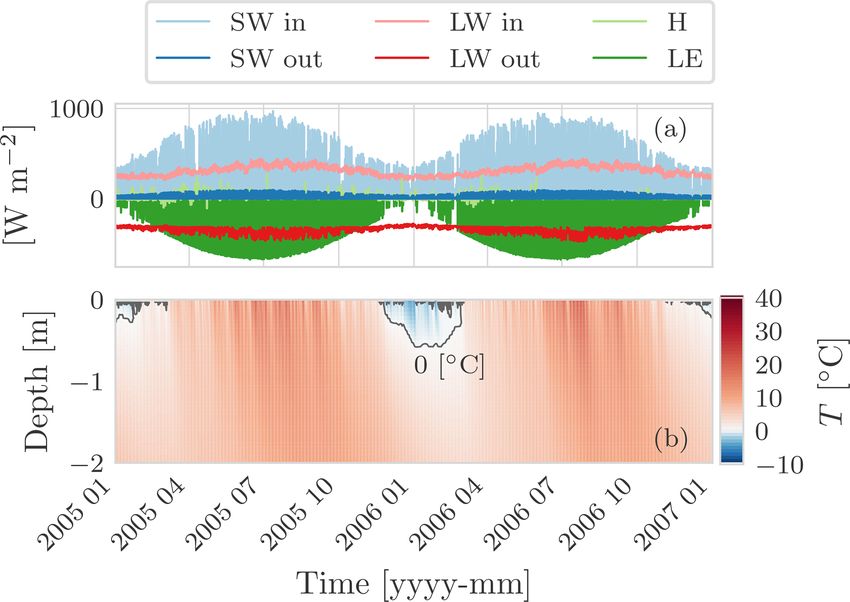
N. Tubini and R. Rigon: WHETGEO-1D                                                                                                  79

that ensure the conservation of mass and energy for any time         itself depends on ψ and so is not constant over a discrete
step size and for a great variety of conditions. It is interesting   time interval during which ψ changes value. Let us discretize
to note that some of these algorithms were presented almost          the time derivative in Eq. (11) by using the backward Euler
a decade ago in the math community, remaining a little con-          scheme and obtain
cealed, however. Although WHETGEO is meant to deal with                 ψin+1 − ψin
the transport of solutes and tracers, this topic will be cov-        c̃i             ,                                           (13)
                                                                            1t
ered in a dedicated paper since its physics and numerics are
slightly different from those of the water and energy budgets.       where c̃i is the discrete operator of the soil moisture capacity,
   Moreover, WHETGEO-1D represents the first brick of a              c(ψ). In order to preserve the chain rule of derivatives at the
new expandable land-surface model (Bisht and Riley, 2019):           discrete level, i.e. the equality c∂ψ/∂t = ∂θ (ψ)/∂t, c̃i has to
the forthcoming development of WHETGEO-1D and its in-                satisfy the requirement (Roe, 1981)

clusion in the GEO-SPACE (Soil Plant Atmosphere Contin-              c̃i ψin+1 − ψin = θ ψin+1 − θ ψin .

                                                                                                                                 (14)
uum Estimator) model that aims to simulate the soil–plant
continuum (D’Amato et al., 2022).                                    As can be seen from the above equation, the right definition
   In the following section we discuss the mathematical is-          of c̃i depends on the solution itself. To overcome this prob-
sues and the numerics of our implementation. In the subse-           lem, in the literature different techniques have been presented
quent one, we describe the informatics and software engi-            to improve the evaluation of c̃i , but none ensures mass con-
neering issues, as well as how we solved them. Finally, we           servation (Farthing and Ogden, 2017).
discuss WHETGEO-1D implementation by testing it against                 There is a third form of Eq. (2), the so-called “θ -based
some analytical solutions available for simplified parameter-        form”, that reads as
izations and boundary conditions; for details of these see Ap-       ∂θ
pendix C.                                                                 = ∇ · [D(θ )∇θ + K(θ )] ,                             (15)
                                                                      ∂t
                                                                     where all is made explicit by inverting the SWRC, and
2     Mathematical issues and numerics                               D(θ ) = K(θ )∂ψ/∂θ is the soil water diffusivity [L2 T−1 ].
                                                                     The first term on the right-hand side represents the water
Translating these equations into numerical discretized codes         flow due to capillary forces, while the second term is the con-
implies overcoming some challenges, as we illustrate in the          tribution due to gravity (Farthing and Ogden, 2017). The θ -
next sections by exploring, at first, the issues posed by each       based form is mass-conserving, and it can be solved perfectly
of the equations.                                                    by mass conservative methods (Casulli and Zanolli, 2010).
                                                                     However, its applicability is limited to the unsaturated zone
2.1    General issues of the R 2 equation                            since water content varies between θr and θs , whereas wa-
                                                                     ter suction is not bounded. This formulation is intrinsically
Equation (2) is said to be written in “mixed form” because           not suited to fulfilling our Requirement III. Moreover, water
it is expressed in terms of θ and ψ (and uses the SWRC to            content is discontinuous across layered soil since the SWRCs
connect the two variables).                                          are soil-specific, whereas water suction is continuous even
   The “ψ-based form” is derived from Eq. (2) by applying            in inhomogeneous soils (Farthing and Ogden, 2017; Bonan,
the chain rule for derivatives:                                      2019).
       ∂ψ                                                               In WHETGEO, we directly use the conservative form of
c(ψ)      = ∇ · [K(ψ)∇(ψ + z)] ,                             (11)    the R 2 equation, Eq. (2), which seems the easiest way to deal
       ∂t
                                                                     with both the mass conservation issues and the extension of
where
                                                                     the equation to the saturated case.
          ∂θ (ψ)
c(ψ) =           ,                                           (12)    2.1.1        The discretization of the R 2 equation
           ∂ψ
with dimension [L−1 ] as the specific moisture capacity, also        The implicit finite-volume discretization of Eq. (2) reads as
called hydraulic capacity. Even though Eqs. (2) and (11) are
                                                                                                           ψ n+1 − ψin+1
analytically equivalent under the assumption that the water          θi (ψin+1 ) = θi (ψin ) + 1t K n+11 i+1             + K n+11
                                                                                                     i+ 2     1zi+ 1          i+ 2
content is a differentiable variable, this is not generally true                                                    2
in the discrete domain where the derivative chain rule is not                                 ψ n+1 − ψi−1n+1
always valid (Farthing and Ogden, 2017). Because of this                           − K n+11 i                  − K n+11 + Sin ,    (16)
                                                                                        i− 2     1zi− 1            i− 2
the ψ-based form may suffer from large balance errors in                                               2
the presence of big nonlinearities and strong gradients, as          where 1t is the time step size,
discussed in Casulli and Zanolli (2010), Farthing and Og-                Z
den (2017), Zha et al. (2019), and literature therein. The spe-      Si = S d                                                    (17)
cific moisture capacity c, which appears in the storage term,                i

https://doi.org/10.5194/gmd-15-75-2022                                                         Geosci. Model Dev., 15, 75–104, 2022
80 N. Tubini and R. Rigon: WHETGEO-1D
is an optional source–sink term in volume, and θi (ψ) is the
ith water volume given by
Z
θi (ψ) = θ (ψ) d. (18)
i
Equation (16) can be written in matrix form as
θ (ψ) + Tψ = b, (19)
where ψ = {ψi } is the tuple of unknowns, θ(ψ) = θi (ψi )
is a tuple function representing the discrete water volume,
T is the flux matrix, and b is the right-hand-side vector of
Eq. (16), which is properly augmented by the known Dirich-
let boundary condition when necessary. For a given initial
condition ψi0 , at any time step n = 1, 2, . . ., Eq. (16) con-
stitutes a nonlinear system for ψin+1 , with the nonlinearity
affecting only the diagonal of the system and being repre- Figure 1. Scheme of the computational domain to solve the R 2
sented by the water volume θi (ψin+1 ). This set of equations is equation in 1D. The uppermost node represents the water depth at
a consistent and conservative discretization of Eq. (2). There- the soil surface. By considering this additional computational node
fore, regardless of the chosen spatial and temporal resolution, the boundary condition does not change its nature depending on the
ψin+1 is a conservative approximation of the new water suc- solution.
tion.
soil surface.
2.1.2 Surface boundary condition n+1 n+1
n+1 n ψN −ψN −1
HN (ψN ) − 1t 0 − K 1 1z 1
N− 2
N− 2
The definition of the type of surface boundary condition
(Neumann vs. Dirichlet) for the R 2 equation is a nontrivial n n n
= HN (ψN ) + 1t J − K 1 if i = N
N− 2
task since it can depend on the state of the system. In the lit- " n+1
# (21)
ψi+1 − ψin+1 ψin+1 − ψi−1
n+1
θi (ψin+1 ) − 1t
n n
erature several approaches are used (Furman, 2008). These
Ki+ 1 − Ki− 1
2 1zi+ 1 2 1zi− 1
approaches are mainly based on a switch of the type of the
2 2
= θi (ψin ) + 1t Ki+
n n
boundary condition from a prescribed head to prescribed flux 1 − Ki− 1
if i = 1, 2, . . ., N − 1
2 2
and vice versa. This switching often causes numerical diffi-
culties that need to be addressed (Furman, 2008). Here, J n is the rainfall intensity and represents the Neumann
To overcome this problem we have included an additional boundary condition used to drive the system at the soil sur-
computational node at the soil surface. As will be made clear face. For any time step, Eq. (21) can be written in matrix
in the following, for it we prescribe an “equation state” like form, similar to (Eq. 19), as
that presented in Casulli (2009):
V (ψ) + Tψ = b, (22)
where ψ = {ψi } is the tuple of unknowns, V (ψ) = (θi (ψi ))
(
ψ if ψ > 0
H (ψ) = (20) for i = 1, 2, . . ., N − 1, VN (ψ) = H (ψ) is a tuple function
0 otherwise,
representing the discrete water volume, T is the flux matrix,
and b is the right-hand-side vector of Eq. (16), which is prop-
where H [L] is the water depth, which also represents the erly augmented by the known Dirichlet boundary condition
pressure if the ponding is assumed to happen in hydrostatic when necessary. For a given initial condition ψi0 , at any time
conditions. By doing so, it is possible to prescribe as the step n = 1, 2, . . . Eq. (22) constitutes a nonlinear system for
surface boundary condition the rainfall intensity (Neumann ψin+1 , with the nonlinearity affecting only the diagonal of the
type) without resorting to any switching techniques to repro- system and being represented by the water volume Vi (ψin+1 ).
duce infiltration excess or saturation excess processes. In this Therefore, regardless of the chosen spatial and temporal res-
case the system in Eq. (19) must be modified to account for olution, ψin+1 is a conservative approximation of the new wa-
the additional computational node describing the state of the ter suction.
Geosci. Model Dev., 15, 75–104, 2022 https://doi.org/10.5194/gmd-15-75-2022
N. Tubini and R. Rigon: WHETGEO-1D                                                                                                81

2.2     Heat transport numerics issues                               equations. However, once freezing and thawing processes are
                                                                     considered, the heat equation is fully coupled with the R 2
Equation (9) is said to be written in conservative form and          equation, as in Dall’Amico et al. (2011) for instance, and the
expresses an important property, which is the conservation           enthalpy function becomes nonlinear. At this point, since the
of the scalar quantity, in this case the specific enthalpy. It is    enthalpy function is nonlinear the NCZ algorithm is required
interesting to note that by making use of the mass conserva-         to linearize it, as shown in Tubini et al. (2021b). So far, we
tion equation (Eq. 2), Eq. (9) can be written in an analytically     have not considered the problem of water flow in freezing
equivalent form, the so-called nonconservative form (Sopho-          soils; however, being aware of this issue is important for the
cleous, 1979; Šimůnek et al., 2005):                                future developments and code design.
   ∂T
cT      = λ∇ 2 T − ρw cw Jw ∇T .                          (23)       2.2.2     Driving the heat equation with the surface energy
    ∂t
                                                                               budget
   Equation (23) expresses another important property, which
is the maximum principle (Casulli and Zanolli, 2005); i.e.           At the soil surface the heat equation is driven by the sur-
the analytical solution is always bounded, above and below,          face energy balance. The heat flux exchanged between the
by the maximum and minimum of its initial and boundary               soil and the atmosphere, the surface heat flux, F [M T−3 ], is
values, as shown in Greenspan and Casulli (1988, chap. 7.3).         given as
   Although Eqs. (9) and (23) are analytically equivalent,
once they are discretized the corresponding numerical solu-          F = Sin − Sout + Lin − Lout + H − LE,                       (26)
tion will, in general, either be conservative or satisfy a dis-
crete max–min property (Casulli and Zanolli, 2005), but not          where Sin is the incoming shortwave radiation, Sout is the
both as would be required.                                           outgoing shortwave radiation, Lin is the incoming longwave
   As in the case of the water flow, thermal budget issues           radiation, Lout is the outgoing longwave radiation, and H and
can be subdivided into three aspects: the discretization of the      LE are respectively the turbulent fluxes of sensible heat and
equation, the inclusion of the appropriate boundary condi-           latent heat. Fluxes are positive when directed toward the soil
tions, and the implementation of some closure equation for           surface and all have the dimension of an energy per unit area
the thermal capacity and conductivity.                               per unit time [M T−3 ].
                                                                        Similarly to the definition of the surface boundary condi-
2.2.1    The discretization of the heat equation                     tion for the water flow, the surface boundary condition for the
                                                                     energy equation is also system-dependent. In fact, in Eq. (26)
The key feature (Casulli and Zanolli, 2005) to obtaining a           the only fluxes that do not depend on the soil temperature
numerical solution for the heat transport equation that is both      and/or moisture are the incoming shortwave and longwave
conservative and possesses the max–min property is to solve          radiation fluxes, Sin and Lin . The outgoing shortwave radia-
the conservative form of the heat equation by using the veloc-       tion flux is usually parameterized as
ity field obtained in solving the continuity equation (Eq. 2).
By making use of the upwind scheme for the advection part            Sout = αSin ,                                               (27)
and the centred difference scheme for the diffusion part we
have                                                                 where the surface albedo α [−] can be assumed to vary with

                                       1 n+1  n+1                  the soil moisture content (Saito et al., 2006) and radiation
CTn+1  T i
          n+1
              = C  n n
                     T
                   Ti i  − ρ   c
                             w w  1t    J 1 Ti+1 + Tin+1             wavelength. The outgoing longwave surface radiation is
   i                                   2 1+ 2
       1                                                             Lout = (1 − )Lin + σ Ts4 ,                                (28)

   − J n+11 Ti+1     n+1
                         + Tin+1
       2 1+ 2
                                                                   where Ts [2] the temperature of the topmost layer of soil,  is
       1 n+1  n+1          n+1
                                  1
                                         n+1

                                                 n+1       n+1
   − J 1 Ti             + Ti−1 + J 1 Ti+1 + Ti                       the soil emissivity, and σ is the Stefan–Boltzmann constant.
       2 1− 2                        2 1− 2                          The sensible heat flux H is taken as
           "         n+1      n+1            n+1      n+1
                                                          #
                  T i+1  − T i             Ti    − T i−1                     ρa ca
   + 1t λni+ 1                    − λni− 1                  , (24)   H=            (Ta − Ts ),                                   (29)
                2       1z               2      1z                            rH
where                                                                where ρa is the air density [M L−3 ], and ca is the thermal
        Z
CTi =         ρsp csp (1 − θs ) + ρw cw θ (ψ) d.            (25)    capacity of air per unit mass [L2 T−2 2−1 ]. Regarding the
                                                                     aerodynamic resistances rH [T L−1 ], it should be noted that
         i
                                                                     it can be evaluated with different degrees of approximation
When the heat equation does not consider water phase                 and may require a specific modelling solution. For instance,
changes, it is decoupled from the R 2 equation and the finite-       the aerodynamic resistance rH can be evaluated with models
volume discretization leads to a linear algebraic system of          ranging from semi-empirical models to the Monin–Obukhov

https://doi.org/10.5194/gmd-15-75-2022                                                           Geosci. Model Dev., 15, 75–104, 2022
82                                                                                         N. Tubini and R. Rigon: WHETGEO-1D

similarity (Liu et al., 2007) or even by solving the turbulent      ent (Shewchuk, 1994). These algorithms are well known and
dynamics with direct methods (Raupach and Thom, 1981;               do not need to be explained here.
Mcdonough, 2004).                                                      However, the reduction of a nonlinear system to a linear
   The latent heat flux is taken here as given by a formula of      one is not trivial. We illustrate the issues by taking the R 2
the type                                                            equation as an example. As discussed in depth in Zha et al.
                                                                    (2019), Farthing and Ogden (2017), and references therein,
               rH rv                                                the linearization of the R 2 equation is challenging. Following
LE = lρa EP           ,                                     (30)
              rH + rv                                               the work of Celia et al. (1990), a lot of advancements have
                                                                    been made in this direction: Hydrus, CATHY, and ParFlow
where l [M L2 T−2 ] is the specific latent heat of vaporization     use variants of the Newton and Picard iteration methods (Zha
of water, EP is the potential evapotranspiration, and rH and        et al., 2019; Paniconi and Putti, 1994), while GEOtop 2.0
rv [T L−1 ] are respectively the aerodynamic resistance and         implements a suitable globally convergent Newton method
the soil surface resistance to water vapour flow. The latent        (Kelley, 2003). Although current algorithms are relatively
heat flux it is the sum of two distinct processes: evapora-         stable, they may fail to converge or require a considerable
tion and transpiration. Compared to the other fluxes, latent        computational cost (Zha et al., 2019). This has significant im-
heat flux presents further complications because evaporation        pacts on both the reliability of the solution, which can have
is both an energy- and a water-limited process, and transpira-      mass balance errors, and the computational cost to produce it
tion also depends on the physiology of trees (as well as root       (Farthing and Ogden, 2017; Zha et al., 2019). Since Casulli
distribution and growth and leaf cover). The latent heat flux       and Zanolli (2010) and Brugnano and Casulli (2008), a new
is associated with the water flux that must be accounted for        method was found, called nested Newton by the authors and
in the R 2 equation. Here we present a simplified treatment         NCZ in the following, that guarantees convergence in any
of the latent heat flux as an external driving force and/or pre-    situation, even with the use of large time steps and grid sizes.
scribed boundary condition. A more exhaustive and physi-               As clearly pointed out by Casulli and Zanolli (2010),
cally based treatment of the latent heat flux, and the related      what makes the linearization of the R 2 equation difficult
water flux, is addressed in the ongoing development of the          is the nonmonotonic behaviour of the soil moisture capac-
GEO-SPACE model (D’Amato, 2021).                                    ity. A mathematical proof of convergence for NCZ exists
   Including the surface energy budget boundary condition           (Brugnano and Casulli, 2008, 2009; Casulli and Zanolli,
requires the computation of additional quantities such as           2010, 2012), which is not repeated here. However, we take
the incoming radiation fluxes, the shortwave radiation and          the time to illustrate this new algorithm with care.
the longwave radiation, and the potential evapotranspiration           Let us start again from the nonlinear system (Casulli and
flux. These quantities can be easily computed within the            Zanolli, 2012):
GEOframe system in which WHETGEO-1D is embedded.
The proper estimation of the incoming radiation fluxes is           V (ψ) + Tψ = b,                                            (31)
far from being a simple task, and it is often oversimpli-
fied in hydrological problems. Our approach is to use the           where ψ = (ψi ) is the tuple of unknowns, V (ψ) = (Vi (ψi ))
tools already developed inside the system GEOframe, which           is a non-negative vectorial function, and the Vi (ψi ) terms are
were tested independently and accurately (Formetta et al.,          defined for all ψi ∈ R and can be expressed as
2013, 2014a). Similarly, the evapotranspiration can be com-
puted with other GEOframe components (Bottazzi, 2020;                            Zψi
Bottazzi et al., 2021).                                             Vi (ψi ) =         ai (ξ ) dξ.                             (32)
                                                                             −∞
2.3   Algorithms
                                                                    For all i = 1, 2, . . ., N , the following assumptions are made
By using a numerical method, here the finite-volume method,         for the functions ai (ψ) (we are quite literally following Ca-
a partial differential equation is transformed into a system        sulli and Zanolli, 2010 here):
of nonlinear algebraic equations, as has already been shown.
                                                                    A1: ai (ψ) is defined for all ψ ∈ R and is a non-negative
The system has to be solved with iterative methods, and, at
                                                                        function with bounded variations;
their core, these reduce the problem to using a linear sys-
tem solver. The solver can be of various types, according to        A2: ψi∗ ∈ R exists such that ai (ψ) is strictly positive
the dimension of the problem. For instance, in 1D, the final            and nondecreasing in (−∞, ψi∗ ) and nonincreasing in
system of finite-volume problems we present is tridiagonal              (ψi∗ , +∞).
and can be conveniently solved with the Thomas algorithm
(Quarteroni et al., 2010), which is a fast direct method. In 2D     T in Eq. (31) is the so-called matrix flux, and it is a symmet-
or 3D, the final matrix is not tridiagonal, and a different solu-   ric and (at least) positive semi-definite matrix satisfying one
tion method must be used: for instance, the conjugate gradi-        of the following properties:

Geosci. Model Dev., 15, 75–104, 2022                                                         https://doi.org/10.5194/gmd-15-75-2022
N. Tubini and R. Rigon: WHETGEO-1D                                                                                                          83

T1: T is a Stieltjes matrix, i.e. a symmetric M matrix, or                    vectorial function is defined as V (ψ) = (θi (ψi )) for i =
                                                                              1, 2, . . ., N − 1 and VN (ψ) = H (ψ). Therefore, the nonlin-
T2: T is irreducible, null(T) ≡ span(v), with v > 0 (compo-                   ear system in Eq. (38) is valid to describe both the subsur-
    nentwise), and T+D is a Stieltjes matrix for all diagonal                 face and surface waters when the symbols are appropriately
    matrices D O, with O denoting the null matrix.                            understood.
Finally, b is the vector of the known terms. When T satisfies                    This aspect, the use of two different equation states, and
property T2, then for Eq. (31) to be physically and mathe-                    the fact that the NCZ algorithm can be successfully re-used
matically compatible, the following assumption about b is                     to solve other problems (Casulli and Zanolli, 2012; Tubini et
required:                                                                     al., 2021b), requires a careful design of its implementation,
                                                                              as discussed in the following sections.
0 < v | b < v | V Max ,                                   (33)
                   +∞
where V Max = −∞ ai (ξ )dξ .
                 R
                                                                              3     Design and deployment of WHETGEO-1D
  Having assumed that the ai (ψ) terms are non-negative
functions of bounded variations, they are differentiable al-                  The concepts and requirements previously illustrated must
most everywhere, admit only discontinuities of the first kind,                be cast into software whose usability, expandability, and in-
and can be expressed as the difference of two non-negative,                   spectability are demanded by good software design, which
bounded, and nondecreasing functions, say pi (ψ) and qi (ψ),                  adds further requirements. The software design requirements
such that                                                                     and the software deployment are explained below.

ai (ψ) = pi (ψ) − qi (ψ) ≥ 0                                           (34)   3.1    Design requirements
0 ≤ q(ψ) ≤ p(ψ)
                                                                              One of the major difficulties encountered by a research group
for all ψ ∈ R. When a(ψ) terms satisfy assumptions A1                         concerns the development and re-use of scientific software
and A2, the corresponding decomposition (known as the Jor-                    (Berti, 2000) and the writing of structurally clean code, i.e.
dan decomposition as in Chistyakov, 1997, and presented in                    a code that is easily readable and understandable, with ob-
Fig. 2) is given by                                                           jects that have a specified and possibly unique responsibility
                                                                              (Martin, 2009).
 pi (ψ) = ai (ψ)         qi (ψ) = 0                     if ψ ≤ ψi∗               An object-oriented programming approach, with the adop-
 pi (ψ) = ai (ψi∗ )      qi (ψ) = pi (ψ) − ai (ψ)       if ψ > ψi∗ ,          tion of standard design patterns (DPs) (Gamma et al., 1995;
                                                                       (35)   Freeman et al., 2004) and the creation of new ones, has been
                                                                              adopted for the internal class design and hierarchy.
where ψi∗ is the position of the maximum of pi . Thereafter,                     The design principles followed by the WHETGEO-1D
V (ψ) can be expressed as                                                     software can be summarized as follows.
V (ψ) = V 1 (ψ) − V 2 (ψ),                                             (36)       a. The software should be open-source to allow inspection
                                                                                     and improvements by third parties.
where the ith component of V 1 (ψ) and V 2 (ψ) is defined as

               Zψi                               Zψi                              b. For the same reason it should be organized into parts,
                                                                                     each with a clear functional meaning and possibly a sin-
V1,i (ψi ) =         pi (ξ ) dξ   V2,i (ψi ) =         qi (ξ ) dξ.     (37)
                                                                                     gle responsibility.
            −∞                               −∞

  By making use of Eq. (36) the algebraic system in Eq. (31)                      c. The software can be extended with minimal effort and
can be written as                                                                    without modifications (according to the “open to ex-
                                                                                     tensions, closed to modifications” principle; Freeman
V 1 (ψ) − V 2 (ψ) + Tψ = b.                                            (38)          et al., 2004). In particular, the parts to be modified are
                                                                                     those that, according to the discussion in the previous
   It is necessary here to point out exactly how the nonlin-                         sections, could be changed to try new closures, i.e. the
ear system in Eq. (31) reads when considering only the R 2                           SWRCs and the hydraulic conductivities in the case of
equation and when the water depth function is used to prop-                          the R 2 equation and the thermal capacity and thermal
erly define the surface boundary condition. In the first case,                       conductivity in the case of the energy budget. Adding a
i.e. when Neumann or Dirichlet boundary conditions are                               new SWRC type or a new conductivity function should
used, the vectorial function is defined as V (ψ) = (θi (ψi ))                        be easy.
for i = 1, 2, . . ., N .
   Instead, when we consider the water depth function to                          d. The largest set of boundary conditions should be
describe the computational node at the soil surface, the                             smoothly manageable.

https://doi.org/10.5194/gmd-15-75-2022                                                                Geosci. Model Dev., 15, 75–104, 2022
84                                                                                      N. Tubini and R. Rigon: WHETGEO-1D

Figure 2. Graphical representation of the Jordan decomposition for soil water content using the SWRC model by Van Genuchten (1980) for
a clay loam soil (Bonan, 2019). (a) The Jordan decomposition of c(ψ) as in Eq. (35). For ψ = ψ ∗ , c(ψ) presents a maximum: for ψ < ψ ∗
it is increasing, and for ψ > ψ ∗ it is decreasing. This nonmonotonic behaviour causes problems when solving the nonlinear system. c(ψ)
is thus replaced by p(ψ) (in green) and q(ψ) (in blue), which are two monotonic functions whose difference is the original function c.
Consequently, (b) θ (ψ) is replaced by θ1 (ψ) and θ2 (ψ) (Eq. 36).

  e. The implementation of equations should be abstract,                   as much of the code as possible should be shared across
     according to the principle of “programming to inter-                  these. In particular, the NCZ and Newton algorithms
     faces and not to concrete classes”, which is the core                 should be shareable across the various applications.
     of contemporary OOP (Gamma et al., 1995). The dif-
     ferent equations describing the processes should be im-          This requirement implies that the geometry of the domain,
     plemented within the set of classes by implementing a            as well as the topology, should be specified in an abstract
     common interface.                                                manner to cope with the specifics of each dimensionality.
                                                                         The rest of this section is organized to respond to points (a)
  f. The implementation of algorithms should not depend on            to (h). Point (a) is actually responded to in the next section
     the data formats of inputs and outputs.                          describing where the software can be downloaded and with
   Another requirement has to do with the user experience. In         which open license. Points (b) and (c) are accomplished by
fact, solvers of partial differential equations (PDEs) (Menard        studying an appropriate design of classes and the use of de-
et al., 2020) tend to be complex to understand and run when           sign patterns (Gamma et al., 1995; Freeman et al., 2004). For
features are added. In particular, the number of inputs grows         (d), generic programming is used and specific classes are im-
exponentially when features are added, and the user has to            plemented. Point (e) is resolved by deploying a set of classes
overcome a steep learning curve before being able to use              that implement a common interface with an extension that
these software packages to appreciate all the cases imple-            allows it to obtain the required functionalities.
mented and their physics.                                                To respond to the issues raised in (f) and (g), WHETGEO-
                                                                      1D is implemented as various components of OMS3, as
  g. To simplify this situation, WHETGEO-1D has to be im-             shown below, each one with its own inputs. Therefore, the
     plemented is such a way that any of the alternative im-          number of flags to check and the number of unused inputs are
     plementations must come only with their own parame-              reduced to the minimum required by the solvers and parame-
     ters and variables, as well as appear to the user to be as       terizations that the user chooses. If users want to solve the R 2
     simple as possible, though not too simple.                       equation alone, for instance, they can pick out the appropri-
                                                                      ate component and do not need to know about the inputs and
     There is finally a last requirement to consider.
                                                                      details of the energy budget. The separation into components
  h. For computational and research purposes, there will be           has two other advantages. First, it eases the testing of a sin-
     one-, two-, and three-dimensional (1D, 2D, 3D) imple-            gle process against available analytical solutions and against
     mentations of the aforementioned equations. Therefore,           other model results (Bisht and Riley, 2019). Second, it im-

Geosci. Model Dev., 15, 75–104, 2022                                                      https://doi.org/10.5194/gmd-15-75-2022
N. Tubini and R. Rigon: WHETGEO-1D 85
proves the model structure, facilitating the representation of Similarly, we grouped the classes that solve linear and non-
new processes (Clark et al., 2021). linear algebraic systems, containing the Thomas conjugate
Point (h) is solved by deploying new components for the gradient and the various Netwon types of algorithms, into a
1D, 2D, and 3D cases. In the following section we mainly second stand-alone library. The third group of classes gath-
deal with points (b) to (e). Before discussing details of some ers the concrete implementations and the variety of OMS3
classes, a few general choices have to be reported. Data of components that are deployed.
any type are stored internally in vectors of doubles, which The classes used, and their repository for third-party in-
in turn encapsulated in appropriate Java objects. OOP good spection, are illustrated in the 00_Notebooks referred to in
practice would suggest that an object should be immutable Sect. 4 and in the Supplement. However, there are three piv-
(Bloch, 2001), but we decided that the main classes have to otal groups of classes that we want to mention here: these
be mutable and allocated once forever as singletons (Gamma contain the description of the geometry of the integration do-
et al., 1995; Freeman et al., 2004). This potentially exposes main, the closure equation, and the state equation.
the software to side effects but frees it to allocate new ob-
jects at any time step and decreases the computational burden 3.2.1 Computational domain, i.e. the Geometry class
and memory occupancy generated by deallocating unused
obsolete objects at runtime. This approach may be consid- One of the key aspects to have in a generic solver regards the
ered a specific design pattern for partial differential equation management of the grid and, in particular, the definition of its
solvers. topology, or how grid elements are connected to each other.
In the 1D case the description of the topology is quite simple
3.2 The software organization since it can be implicitly contained in the vector representa-
tion: each element of the vector corresponds to a control vol-
The more visible effect of our choices is that we have built ume of the grid, and it is only connected with the elements
various OMS3 components. preceding and following it. It is worth noting that this ap-
– whetgeo1d-1.0-beta proach is peculiar to 1D problems and cannot be adopted for
the 2D and 3D domains, where, especially when unstructured
– netcdf-1.0-beta grids are used, the grid topology requires a smart implemen-
tation of the incidence and adjacency matrices.
– closureequation-1.0-beta For each control volume it is necessary to store its geomet-
rical quantities, their position and dimension, its variables, its
– buffer-1.0-beta
parameter set, and the form of the equation to be solved there,
– numerical-1.0-beta referred to in the following as “equation state”. The appropri-
ate arrangement of information, together with the internal de-
Internally, the classes are assembled by using some interfaces sign of the classes, allows us to create a generic finite-volume
and abstract classes, since WHETGEO-1D is coded using the solver.
Java language.
In order to improve the re-usability of the Java code we 3.2.2 Closure equations, i.e. the ClosureEquation
adopted a generic programming approach (Berti, 2000) that abstract class
consists of decoupling of algorithm implementations from
the concrete data representation while preserving efficiency. The ClosureEquation class is shown in the Unified
The generic approach has been balanced with domain- Modeling Language (UML) diagram in Fig. 3. As explained
specific ones that can improve the computational efficiency in the Introduction, one of the core concepts of modelling
of the software, as is the case of the previously mentioned water and heat transport in soils is the SWRC. Soil is a multi-
Thomas algorithm used in 1D implementations. phase material, and thus knowledge of its composition is of
Another requirement regards the division of software crucial importance in defining its unsaturated hydraulic con-
classes into three main groups, as the lack of a proper sep- ductivity as well as its thermal properties, specific internal
aration between the parameterization of physical processes energy, and thermal conductivity.
and their numerical solutions has been recognized as one An abstract class, ClosureEquation, is defined
of the weak points of existing land-surface models (Clark to contain only abstract methods that would be over-
et al., 2015b, 2021). One group describes the mathematical– written by the concrete classes implementing it. The
physical problem, the second one implements the numerical ClosureEquation class essentially defines a new data
solution (Berti, 2000), and the third one contains the grow- type. A closer inspection of Fig. 3 reveals that the
ing group of concrete classes. The first group contains the ClosureEquation is composed by aggregation with the
SWRC, as well as hydraulic and thermal conductivity, and Parameter class, which contains all the physical pa-
it forms a stand-alone library since its content can eventu- rameters of the model. Moreover, the Parameter class
ally be re-used in the 2D and 3D version of WHETGEO-1D. is implemented by using the Singleton pattern (Freeman
https://doi.org/10.5194/gmd-15-75-2022 Geosci. Model Dev., 15, 75–104, 202286 N. Tubini and R. Rigon: WHETGEO-1D
et al., 2004). This design pattern is functional to have only only one equation state for the soil water content. The nonlin-
one instance of the Parameter class shared by all the ear solver of the NCZ algorithm must work seamlessly with
ClosureEquation objects and to provide a global point any type of boundary condition used and with any type of
of access to the Parameter instance. equation involved in the problem.
The Simple Factory pattern Let us consider, for example, the case of the R 2 equation
SoilWaterRetentionCurvesFactory accom- with water depth as the surface boundary condition. Figure 5
plishes the task of implementing the concrete classes. By reports the pseudocode for computing the nonlinear func-
preferring polymorphism to inheritance and using the Simple tions in the NCZ algorithm using a procedural approach.
Factory pattern (Gamma et al., 1995; Freeman et al., 2004), When traversing the computational grid we need to resort
the developers can easily include and extend existing code or to an if-else statement to compute the nonlinear func-
new formulations or parameterizations of SWRC. Also, the tion of each control volume: the control volume N repre-
Simple Factory fulfils the dependency inversion principle sents the control volume for the surface water, and in this
(Eckel, 2003), and thus new extensions cannot affect the case we need to use the water depth equation state, H (ψ)
functioning of existing code. The same closure equation, for in Fig. 5. The remaining control volumes represent the soil
instance a particular SWRC, can be used to compute the soil moisture, and for them we need to use the SWRC equa-
water volume when solving the R 2 equation and the specific tion state, θ (ψ) in Fig. 5. The main limit of this approach
enthalpy of the soil when solving the heat equation. is that the computation of the nonlinear functions, H (ψ) and
θ (ψ), is hard-wired into the code of the NCZ algorithm. This
3.2.3 Equation state, i.e. the EquationState class presents a shortcoming for the re-usability of the code since,
as the boundary condition changes and the physical problem
The EquationState class in Fig. 4 contains the im- changes, it is necessary to modify the for loop and the name
plementation of the discretized form of the equation state of the objects computing the nonlinear functions.
of the PDE under scrutiny. It contains a reference to the Adopting the OOP and generic programming approach
ClosureEquation object, the Geometry object, and (Fig. 6), it is possible to implement the NCZ algorithm in
the ProblemVariables object. such a way that enhances its re-usability. The key feature
Notably, the solver of a PDE problem can refer to the is the decoupling of the computational grid from the al-
abstract class and to its abstract object without implying gorithm (data) (Berti, 2000). This is achieved through two
the specific concrete equation to be solved or its concrete elements. The first consists of creating a container of the
parameterizations. Moreover, the compositionality of the objects that deal with the equation states of the problem,
EquationState allows the creation of new solvers from equationState, eS in Fig. 6. Second, we use a label
existing closures without the need to add new subclasses. As equationStateID, eSID in Fig. 6, to specify the be-
shown in the UML in Fig. 4, the EquationState class haviour of each control volume. So, the behaviour of each
defines methods used to linearize the PDE when it is non- control volume is determined by this label and not by the
linear. For instance, it computes the first and second deriva- position of the element in the grid. Specifically, when we tra-
tives and the functions necessary to define the Jordan de- verse the grid we use the equationStateID to determine
composition as required by the NCZ algorithm. Specifically, which object inside the container equationState to use.
these methods are p, q, pIntegral, qIntegral, and The NCZ algorithm has been implemented
computeXStar. in the NestedNewtonThomas class. The
In our code design the ClosureEquation class is lim- NestedNewtonThomas contains a reference to the
ited to computing a physical parameterization, whereas the Thomas object, whose task is to solve a linear system, and
EquationState class is used to discretize the equation to a list of EquationState objects (Fig. 7). Considering
state of the PDE and whenever required to properly linearize the ubiquity of nonlinear problems in hydrology and the
it. Any new concrete EquationState subclass can either robustness of the NCZ algorithm, the NCZ algorithm has
have the same physics of another with a different solver or been encapsulated in a stand-alone library.
different physics with the same solver. The example has been illustrated in 1D, but it becomes
even more effective when working in 2D or 3D, especially
3.3 Generic programming at work with an unstructured grid.
As explained in Sect. 2.1.2, the definition of the surface
boundary condition for the R 2 equation can require the in- 4 Information for users and developers
troduction of an additional computation node at the soil sur-
face to simulate the water depth. This means that we have While most of what has been written so far is of general ap-
two different equation states: one for the soil water content plication, the deployment shown here is 1D. Information on
and one for the water depth. On the other hand, when consid- WHETGEO-1D for users and developers is provided in the
ering the Neumann or Dirichlet boundary condition we have Supplement, where there is a Jupyter Notebook that contains
Geosci. Model Dev., 15, 75–104, 2022 https://doi.org/10.5194/gmd-15-75-2022You can also read